Essais sur l'estimation structurelle de la demande

(1)

HAL Id: tel-02373983

https://tel.archives-ouvertes.fr/tel-02373983

Submitted on 21 Nov 2019

HAL is a multi-disciplinary open access

archive for the deposit and dissemination of sci-entific research documents, whether they are pub-lished or not. The documents may come from teaching and research institutions in France or abroad, or from public or private research centers.

L’archive ouverte pluridisciplinaire HAL, est destinée au dépôt et à la diffusion de documents scientifiques de niveau recherche, publiés ou non, émanant des établissements d’enseignement et de recherche français ou étrangers, des laboratoires publics ou privés.

Essais sur l’estimation structurelle de la demande

Julien Monardo

To cite this version:

Julien Monardo. Essais sur l’estimation structurelle de la demande. Economies et finances. Université Paris-Saclay, 2019. Français. �NNT : 2019SACLN042�. �tel-02373983�

(2)

Thèse

de

do

ctorat

NNT

:

2019SA

CLN042

Thèse de doctorat de l’Université Paris-Saclay

préparée à l’École normale supérieure Paris-Saclay Ecole doctorale n◦578 Sciences de l’homme et de la société (SHS)

Spécialité de doctorat : Sciences économiques

Thèse présentée et soutenue à Cachan, le 18 octobre 2019, par

Julien Monardo

Composition du Jury :

Debopam Bhattacharya

Professeur associé, University of Cambridge Rapporteur Alfred Galichon

Professeur, New York University Rapporteur Steven Berry

Professeur, Yale University Président Xavier d’Hautfœuille

Administrateur Hors Classe, INSEE (CREST) Examinateur Laura Grigolon

Professeur assistant, University of Mannheim Examinateur André de Palma

(3)

Remerciements

J’aimerais commencer cette thèse en consacrant quelques mots aux personnes sans lesquelles cette thèse n’aurait pas été possible.

Mes premiers remerciements vont à mon directeur de thèse, André de Palma, pour ses conseils et son soutien durant ces trois années. Je lui suis très reconnais-sant de m’avoir fait bénéficier de son expertise et de son expérience, notamment à travers la co-écriture du premier chapitre de cette thèse. Les nombreuses dis-cussions que nous avons eues m’ont beaucoup appris.

Je tiens également à remercier tous les membres de mon jury : Debopam Bhat-tacharya et Alfred Galichon d’avoir accepté la charge de rapporteur ; ainsi que Steven Berry, Xavier d’Hautfœuille et Laura Grigolon d’avoir accepté d’être mem-bres de mon jury.

Je souhaiterais également remercier toutes les personnes avec lesquelles j’ai eu la chance de travailler. Tout d’abord, Alessandro Iaria qui m’a initié à l’économie industrielle empirique à l’ENSAE et au CREST et qui m’a donné envie de faire cette thèse ; ensuite, Mogens Fosgerau avec qui j’ai pris plaisir à co-écrire et pour son accueil chaleureux durant mes deux séjours à l’université de Copenhague le premier chapitre de cette thèse ; Ao Wang avec qui j’ai partagé de nombreuses discussions passionnantes ; et Nathalie Picard avec laquelle je partage un projet en économie de la famille.

Je suis tout particulièrement reconnaissant envers Morgane Cure pour son soutien, ses conseils et sa bienveillance, et envers Hugo Molina pour son sou-tien, ses conseils et les conversations interminables que nous avons eues. Leur présence au cours de ces trois dernières années a été précieuse.

Je souhaiterais ensuite remercier ceux avec qui j’ai eu l’honneur de partager mes bureaux à l’ENS Paris-Saclay et au CREST : Bastien Alvarez, Rémi Avignon, Florian Bonnet, Etienne Chamayou, Morgane Guignard, Juan Daniel Hernandez, Alessandro Ispano, Manuel Marfan Sanchez, Emmanuel Paroissien, Marine Sales, Benjamin Walter, Jiekai Zhang.

Je remercie également toutes les personnes de l’ENS Paris-Saclay et du CREST avec lesquelles j’ai partagé ces trois dernières années, les chercheurs, doctorants, stagiaires, et membres du personnel administratif. En particulier, je remercie Laurent Linnemer et Emmanuelle Taugourdeau pour la bienveillance dont ils ont fait preuve à mon égard. Je souhaite en particulier remercier Marie-Laure Al-lain, Christophe Bellego, Marie-Laure Cabon-Dhersin, Arthur Cazaubiel, Claire

(4)

Laﬃtte, Alexis Larousse, Morgane Le Breton, Samuel Ligonnière, François Pan-nequin, Jean-Christophe Tavanti, Farid Toubal, Thomas Vendryes, Thibaud Vergé.

Ma thèse a également bénéficié des discussions avec plusieurs doctorants et chercheurs, en particulier Steven Berry, Xavier d’Hautfœuille, Yannick Guyonva-rch, Olivier de Groote, Ali Horstascu, Jonas Lieber, Laurent Linnemer et Aureo de Paula.

Je remercie également mes collègues de Telecom ParisTech qui m’ont accueilli en post-doc au sein du département SES, notamment Marc Bourreau, Lukasz Grzybowski et Christine Zulehner. J’en profite aussi pour remercier Marie-Laure Allain, Roxana Fernandez, Xavier d’Hautfœuille et Farid Toubal pour leur aide précieuse dans l’obtention de ce post-doc.

Enfin, je témoigne toute ma reconnaissance à ma famille et mes amis (hors recherche), en particulier Aurélie Monardo, Florence Monardo, Claire Rougevin-Baville, Louis de Catheu, Guillaume Pommey et Ambroise Pouzoulet.

(5)

Résumé de la thèse

L’estimation structurelle des modèles de demande sur des marchés de produits diﬀérenciés joue un rôle important en économie. Elle permet de mieux com-prendre les choix des consommateurs (e.g., en estimant les élasticités-prix de la demande). De plus, elle est le point de départ de l’étude de plusieurs questions économiques d’intérêt, incluant celles relatives au pouvoir de marché des en-treprises (Berryet al.,1995;Nevo,2001), à la fusion d’entreprises (Nevo,2000), à l’introduction de nouveaux produits sur le marché (Petrin, 2002; Gentzkow,

2007), à la politique commerciale (Goldberg,1995;Verboven,1996;Berryet al.,

1999), et aux taxes (Griﬃth et al.,2019).

La littérature théorique a mis en évidence que les réponses à ces questions dépendent de la forme de la fonction de demande, laquelle est décrite par sa pente et sa courbature. Ainsi, étant donné un modèle d’oﬀre (e.g., modèle sta-tique de concurrence oligopolissta-tique en prix), la qualité des réponses repose sur la capacité du modèle de demande à être "flexible", i.e., sur sa capacité à capter de manière flexible les substitutions qui existent entre les produits.

L’approche standard consiste à spécifier un modèle d’utilité aléatoire addi-tif, à en calculer sa fonction de demande, et à estimer cette dernière en util-isant la méthode développée par Berry (1994). Le modèle d’utilité aléatoire additif est utilisé pour sa capacité à modéliser le comportement de consomma-teurs hétérogènes choisissant parmi un grand nombre de produits diﬀérenciés de manière parcimonieuse et flexible. La méthode de Berry (1994) est utilisée pour estimer des modèles de demande pour des produits qui sont diﬀérenciés de manières observée et inobservée par le modélisateur. Elle résout les prob-lèmes d’endogénéité liés à la présence de termes d’erreurs structurels, lesquels représentent les caractérististiques des produits qui sont inobservées par le mod-élisateur mais observées et valorisées par les entreprises et les consommateurs. Elle consiste à estimer les paramètres structurels de la fonction de demande à partir du système d’équations qui égalise les demandes observées aux deman-des prédites par le modèle. Or, les termes structurels d’erreurs entrent dans ce système de manière non-linéaire, empêchant donc l’utilisation des techniques standards des variables instrumentales. Berry(1994) propose ainsi d’inverser le système afin d’obtenir des équations de demande inverse au sein desquelles les termes d’erreurs structurels entrent de manière linéaire et de les utiliser comme base pour l’estimation. Toutefois, en général, ces demandes inverses n’ont pas

(6)

lèmes connexes d’optima locaux et de précision de l’inversion numérique (Knittel & Metaxoglou,2014).1

La méthode de Berry et al.(1995), connue sous le nom de méthode BLP, est la méthode la plus populaire et la plus avancée de cette approche. Elle utilise un modèle logit à coefficients aléatoires qu’elle estime par un algorithme réal-isant une inversion numérique de la demande, imbriquée dans une procédure d’estimation non-lineaire. Elle permet de capter de manière flexible les substitu-tions entre les produits tout en résolvant les problèmes d’endogénéité. Toutefois, elle est sujette à des difficultés pratiques : la flexibilité exige l’utilisation de nom-breux coefficients qui peuvent être difficiles à identifier empiriquement ; de plus, estimer un modèle logit à coefficients aléatoires peut être difficile et chronophage puisque cela exige l’emploi de procédures d’estimation non-linéaire ainsi que la simulation et l’inversion numérique des fonctions de demande.

L’autre méthode très répandue utilise le modèle logit emboîté, lequel évite les diﬃcultés associées à la méthode BLP en ayant uniquement recours à des régressions linéaires. Toutefois, le modèle logit emboîté est critiqué au motif qu’il ne permet pas de capter de manière flexible les substitutions entre les produits et qu’il demande au modélisateur de définir la structure des nids avant l’estimation, i.e., de déterminer les sources pertinentes de segmentation du marché.

Cette thèse poursuit l’objectif de proposer des modèles de choix des consom-mateurs qui soient flexibles et qui aboutissent à des méthodes d’estimation sim-ples et rapides. Pour cela, elle adopte une approche différente : elle développe de nouveaux modèles de demande inverse qui sont cohérents avec un modèle d’utilité de consommateurs hétérogènes. Cette approche permet de capter de façon flexible les substitutions entre les produits, grâce à de simples régressions linéaires basées sur des données incluant les parts de marché, les prix et les caractéristiques des produits. Ces modèles peuvent être utilisés dans différents domaines de l’économie, incluant l’économie industrielle, le commerce interna-tional et l’économie publique pour, entre autres, mesurer les effets d’une fusion d’entreprise, de l’introduction d’un nouveau produit sur le marché ou d’une nou-velle régulation. Du fait de leur simplicité d’estimation, ces modèles devraient intéresser les chercheurs ainsi que les praticiensantitrust des cabinets de conseil

1_{À ma connaissance, les seuls modèles d’utilité aléatoire additifs ayant une fonction de}

(7)

et des autorités de concurrence qui souhaitent éviter des procédures d’estimation complexes et/ou qui sont pressés par le temps.

Plus spécifiquement, cette thèse développe et étudie des modèles de demande inverse pourJ + 1 produits diﬀérenciés j = 0,...,J de la forme

σj(s)−1= lnGj(s) +c, j = 0, . . . , J,

où s est un vecteur de parts de marché, lnGj est une fonction dont les propriétés restent à définir etc est une constante commune aux diﬀérents produits.

Le premier chapitre de cette thèse construit la classe des modèles general-ized inverse logit (GIL), lesquels sont des modèles de demande inverse de la forme décrite par l’Equation ci-dessus où ln G≡ (lnG₀, . . . , ln GJ) présente des propriétés spécifiques: ln G est telle que G est homogène de degré un et sa matrice jacobi-enne est définie positive et symétrique.2 Ce chapitre montre que chaque mod-èle de cette classe est cohérent avec un modmod-èle de consommateur représentatif et inclut une grande majorité de modèles d’utilité aléatoire additifs. Il four-nit également des méthodes générales pour construire des modèles GIL. Une des méthodes développe des modèles basés sur la construction de nids (i.e., de groupes de produits), lesquels sont analogues à des modèles d’utilité aléatoire additifs qui ont été utilisés à des fins d’estimation de la demande (e.g., le mod-èle logit ordonné de Small (1987) ou le modèle modèle logit emboîté croisé de

Vovsha (1997)). En particulier, il développe le modèle inverse product diﬀeren-tiation logit (IPDL), lequel, de manière analogue au modèle de Bresnahanet al.

(1997), généralise les modèles logit emboîtés, permettant ainsi de capter de façon plus flexible les substitutions entre les produits, y compris de la complémentar-ité. Cette construction présente toutefois deux limites, lesquelles feront l’objet d’une extension dans le deuxième chapitre. D’abord, elle demande au modélisa-teur de choisir la structure des nids avant l’estimation. Ensuite, elle implique que la substitution entre produits ne dépend pas directement des caractéristiques des produits – sauf éventuellement celles utilisées pour la construction des nids.

Le second chapitre développe le modèle flexible inverse logit (FIL), lequel est un modèle GIL qui dépasse les deux limites associées aux modèles basés sur la construction de nids. Le modèle FIL utilise une structure de nids flexible avec un nid pour chaque pair de produits et un paramètre de nid associé (voirChu,

2_{Une fonction}_{f de E dans F est dite homogène de degré un si pour tout x}_{∈ E, pour tout λ > 0,}

f (λx) = λf (x). La matrice jacobienne est la matrice des dérivées partielles du premier ordre d’une

(8)

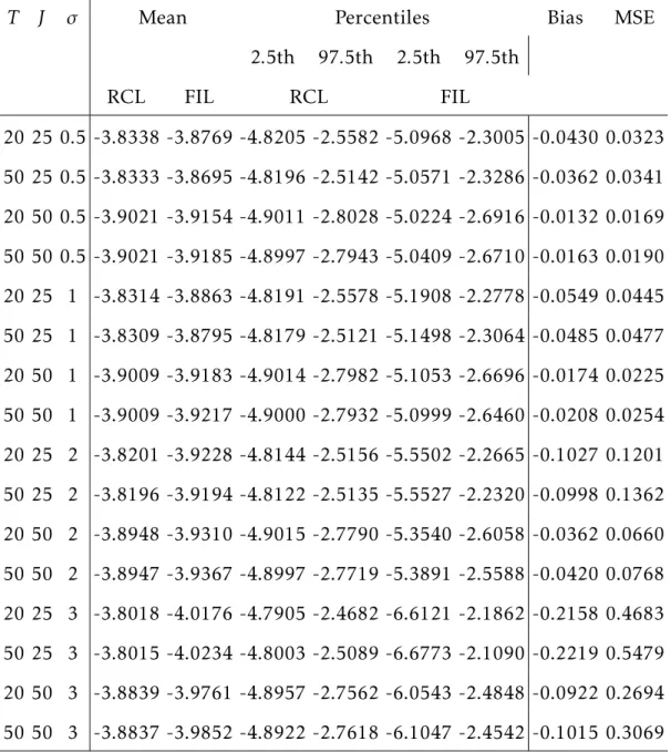
maximisateur d’utilité étudiée parAllen & Rehbeck (2019). Les paramètres de nid du modèle FIL sont ensuite projetés dans l’espace des caractéristiques. Basé sur Pinkse et al. (2002), ces paramètres sont remplacés par une fonction de la distance entre les produits dans l’espace des caractéristiques. Cette projection permet d’obtenir une substitution entre les produits qui dépend directement des caractéristiques des produits, comme c’est le cas du modèle logit à coefficients aléatoires. La projection utilise également les polynômes de Bernstein afin que la manière dont les substitutions dépendent des caractéristiques soit estimée à partir des données et non postulée. Enfin, des simulations de Monte Carlo ont été menés pour mesurer la capacité du modèle FIL à répliquer les élasticités-prix de la demande de modèles logit à coefficients aléatoires pour des spécifications de l’utilité répandues (absence d’effet revenu, utilité linéaire en le prix, un coef-ficient aléatoire normalement distribué, etc.). Les résultats des simulations mon-trent la capacité du modèle FIL à produire des substitutions flexibles.

Le troisième chapitre étudie la micro-fondation du modèle GIL développé dans le premier chapitre de cette thèse. Il montre que les restrictions que le mod-èle GIL impose sur la fonction de demande inverse sont des conditions néces-saires et suﬃsantes de cohérence avec un modèle de consommateurs hétérogènes maximisateur d’utilité, connu sous le nom de perturbed utility model (PUM) et étudié, entre autres, parAllen & Rehbeck (2019). La preuve de ce résultat im-plique deux résultats intermédiaires pouvant être considérés comme intéressants en soi. Tout d’abord, tout PUM génère une fonction de demande qui satisfait une légère variante des conditions de Daly-Zachary (voirDaly & Zachary,1979), laquelle permet de combiner substituabilité et complémentarité en demande. Ensuite, toute fonction de demande satisfaisant ces conditions a une fonction de demande inverse qui est un modèle GIL. Ainsi, par relation d’équivalence, il est montré que les modèles GIL, les PUM et les modèles de demande satisfaisant la variante des conditions de Daly-Zachary fournissent trois modélisations équiva-lentes du comportement des consommateurs.

(9)

Bibliographie

Roy Allen & John Rehbeck. Identification with additively separable heterogene-ity. Econometrica, 87(3):1021–1054, 2019.

Steven Berry, James Levinsohn, & Ariel Pakes. Automobile prices in market equi-librium. Econometrica, 63:841–890, 1995.

Steven Berry, James Levinsohn, & Ariel Pakes. Voluntary export restraints on automobiles: Evaluating a trade policy. American Economic Review, 89(3):400– 430, 1999.

Steven T Berry. Estimating discrete-choice models of product diﬀerentiation. The RAND Journal of Economics, 25:242–262, 1994.

Timothy F Bresnahan, Scott Stern, & Manuel Trajtenberg. Market segmentation and the sources of rents from innovation: Personal computers in the late 1980s. RAND Journal of Economics, pages S17–S44, 1997.

C Chu. A paired combinational logit model for travel demand analysis. In Trans-port Policy, Management and Technology Towards 2001: Selected Proceedings of the Fifth World Conference on Transport Research, pages 295–309. Vol. 4, West-ern Periodicals, Ventura, CA, 1989.

A Daly & S. Zachary. Improved multiple choice models. InDeterminants of Travel Choice, pages 337–357. ed. by D. Hensher and Q. Dalvi (eds), London: Teak-field, 1979.

Peter Davis & Pasquale Schiraldi. The flexible coeﬃcient multinomial logit (fc-mnl) model of demand for diﬀerentiated products. The RAND Journal of Eco-nomics, 45(1):32–63, 2014.

Matthew Gentzkow. Valuing new goods in a model with complementarity: On-line newspapers. The American Economic Review, 97(3):713–744, 2007.

(10)

Pinelopi Koujianou Goldberg. Product diﬀerentiation and oligopoly in interna-tional markets: The case of the us automobile industry. Econometrica, pages 891–951, 1995.

Rachel Griﬃth, Martin O’Connell, & Kate Smith. Tax design in the alcohol mar-ket. Journal of Public Economics, 172:20–35, 2019.

Christopher R Knittel & Konstantinos Metaxoglou. Estimation of random-coeﬃcient demand models: Two empiricists’ perspective. Review of Economics and Statistics, 96(1):34–59, 2014.

Frank S Koppelman & Chieh-Hua Wen. The paired combinatorial logit model: properties, estimation and application. Transportation Research Part B: Method-ological, 34(2):75–89, 2000.

Aviv Nevo. Mergers with diﬀerentiated products: The case of the ready-to-eat cereal industry. The RAND Journal of Economics, 31(3):395–421, 2000.

Aviv Nevo. Measuring market power in the ready-to-eat cereal industry. Econo-metrica, 69(2):307–342, 2001.

Amil Petrin. Quantifying the benefits of new products: The case of the minivan. Journal of political Economy, 110(4):705–729, 2002.

Joris Pinkse, Margaret E Slade, & Craig Brett. Spatial price competition: a semi-parametric approach. Econometrica, 70(3):1111–1153, 2002.

Kenneth A Small. A discrete choice model for ordered alternatives.Econometrica, pages 409–424, 1987.

Frank Verboven. International price discrimination in the european car market. The RAND Journal of Economics, pages 240–268, 1996.

Peter Vovsha. Application of cross-nested logit model to mode choice in tel aviv, israel, metropolitan area. Transportation Research Record: Journal of the Trans-portation Research Board, (1607):6–15, 1997.

(11)

Notice

The three chapters of this dissertation are self-contained research articles. This explains why some information are redundant, and that the term paper is used instead of "chapter". The first chapter of this dissertation is co-authored with Mogens Fosgerau (University of Copenhagen) and André de Palma (CREST, ENS Paris-Saclay, University of Paris-Saclay). Data used in this dissertation, known as the Dominick’s Database, are made freely available by the James M. Kilts Center, University of Chicago Booth School of Business.

(15)

Chapter 1 The Inverse Product Di

ﬀerentiation

Logit Model

1 Introduction

Estimating the demand for diﬀerentiated products is of great empirical relevance in industrial organization and other fields of economics. It is important for un-derstanding consumer behavior and for analyzing major economic issues such as the eﬀects of mergers and changes in regulation. Ideally, one would like to em-ploy a model that accommodates rich patterns of substitution, while requiring just regression for estimation.

This paper proposes the Inverse Product Diﬀerentiation Logit (IPDL) model, which generalizes the nested logit model by allowing richer patterns of substi-tution and in particular complementarity (i.e., a negative cross-price elasticity of demand), while being estimable by linear instrumental variables regression.

The IPDL model is relevant for estimating demands for diﬀerentiated prod-ucts that are segmented along multiple dimensions. It generalizes the nested logit models by allowing the segmentation to be non-hierarchical, which is often desirable in applications. At the same time, it maintains the important advan-tages of the nested logit model. First, its inverse demand has closed form such that numerical inversion of demand is not required. Second, it can be estimated by two-stage least squares regression of market shares on product characteristics and shares related to product segmentation. Third, it is consistent with util-ity maximization. The IDPL model may therefore be an attractive option in the many empirical applications where the nested logit model would otherwise be

(16)

used.

The current practice of the demand estimation literature with aggregate data is to assume an additive random utility model (ARUM) (McFadden,1974) and to estimate it using Berry (1994)’s method to deal with endogeneity of prices and market shares. The logit model is the simplest option, but exhibits the Indepen-dence of Irrelevant alternatives (IIA) property. This implies that an improvement in one product draws demand proportionately from all the other products and makes cross-price elasticities independent of how close products are in charac-teristics space, which is unreasonable in most applications.

The nested logit model with two or more levels generalizes the logit model (see Goldberg, 1995; Verboven, 1996a). This model is commonly used to esti-mate aggregate demand for diﬀerentiated products; some recent examples are

Björnerstedt and Verboven(2016) andBerry et al.(2016). The nested logit model has closed-form inverse demand and is conveniently estimated by two-stage least squares. It imposes, however, the restriction that the segmentation of products, i.e., the nesting structure, must be hierarchical, meaning. that each nest on a lower level must be contained within exactly one nest on a higher level. This severely constrains the substitution patterns that the nested logit model can ac-commodate, since the IIA property still holds within nests and at the nest level. Furthermore, the sequence of segmentation dimensions in the hierarchy is not unique and often not obvious.1

The logit and nested logit models belong to the wider class of Generalized Extreme Value (GEV) models developed by McFadden (1978).2 A number of recent papers have proposed members from this class in order to obtain mod-els with richer substitution patterns. The product diﬀerentiation logit model of

Bresnahan et al.(1997) extends the nested logit model by allowing the grouping of products to be non-hierarchical. The ordered logit model ofSmall(1987) and the ordered nested logit model ofGrigolon(2018) describe markets having a nat-ural ordering of products.3 The seminal paper byBerry et al. (1995) overcomes

1_Hellerstein₍₂₀₀₈_{) writes, concerning the beers market, "[D]emand models such as the}

mul-tistage budgeting model or the nested logit model do not fit this market particularly well. It is diﬃcult to define clear nests or stages in beer consumption because of the high cross-price elastic-ities between domestic light beers and foreign light and regular beers. When a consumer chooses to drink a light beer that also is an import, it is not clear if he categorized beers primarily as domestic or imported and secondarily as light or regular, or vice versa."

2_{GEV models are ARUM in which the random utilities have a multivariate extreme value}

distribution (Fosgerau et al.,2013).

(17)

nonpara-CHAPTER 1. THE INVERSE PRODUCT DIFFERENTIATION LOGIT MODEL

the limitations of the nested logit model by specifying a random coeﬃcient logit model, which breaks IIA at the population level. However, the inverse demands of these more general models do not have closed form.

The richer substitution patterns of these models is obtained at the cost of more complex and time-consuming nonlinear estimation procedures such as the nested fixed point (NFP) approach of Berry et al. (1995) or the Mathematical Program with Equilibrium Constraints (MPEC) approach ofDubé et al. (2012), which are associated with issues of local optima and choice of starting values (see e.g.,Knittel and Metaxoglou,2014).

In this paper, we depart from the standard practice by specifying a model in terms of the inverse demand. Given linear-in-parameters utility indexes, the model can then be directly estimated by linear regression using Berry (1994)’s method. More specifically, we propose the IPDL model for products that are seg-mented along multiple dimensions. The IPDL model extends the nested logit model by allowing arbitrary, non-hierarchical grouping structures (i.e., any par-titioning of the choice set in each dimension). It improves on the nested logit model by allowing for richer patterns of substitution and, as we show, even com-plementarity. This improvement is achieved by removing the constraint that the segmentation should be hierarchical, and it is therefore costless. While the IPDL model requires modelers to define the segmentation, the relative importance of segmentation dimensions can be estimated.

Another important approach in demand estimation is the flexible functional form approach (e.g., the AIDS model ofDeaton and Muellbauer,1980), where the error term has no immediate structural interpretation. By contrast, in this paper, the error term has the structural interpretation ofBerry(1994) that it represents product/market-level characteristics unobserved by the modeller but observed by consumers and firms.

The IPDL model belongs to a wider class of inverse demand models, that we label Generalized Inverse Logit (GIL) models. We show that any GIL model is consistent with a representative consumer model (RCM) in which a utility-maximizing representative consumer chooses a vector of nonzero demands, trad-ing oﬀ variety against quality. We also show that any ARUM is equivalent to some GIL model. However, the converse is not true, since some GIL models ex-hibit complementarity, which cannot occur in an ARUM. We establish a new de-mand inversion result, which extends Berry (1994) and Berry et al. (2013) by metric methods, seeDavis and Schiraldi(2014) for more details.

(18)

allowing complementarity. It is often desirable to allow complementarity as im-portant economic questions hinge on the extent to which products are substitutes or complements. In particular, this directly aﬀects the incentives to introduce a new product on the market, to bundle, to merge, etc.4

The paper is organized as follows. Section 2sets the context, introducing the role of demand inversion with the inverse demand of the logit and nested logit models as examples. Section 3 introduces the IPDL model as a generalization of the inverse demand of the nested logit model and shows how to estimate it with aggregate data. Section4applies the IPDL model to estimate the demand for ready-to-eat cereals in Chicago, finding that complementarity is pervasive in this market. Section 5 introduces the wider class of GIL models. Section 6

studies its linkages with the ARUM and RCM. Section7concludes. A supplement provides Monte Carlo evidence on the IPDL model as well as general methods and examples for building GIL models that go beyond the IPDL model.

2 Motivation

2.1 General Setting: the Role of Demand Inversion

Consider a population of consumers choosing from a choice set of J + 1 di ﬀer-entiated products, denoted byJ = {0,1,...,J}, where products j = 1,...,J are the inside products and product j = 0 is the outside good. We consider aggregate data on market sharessjt > 0, prices pjt ∈ R and K product/market characteris-tics x_jt ∈ RK for each inside productj = 1, . . . , J in each market t = 1, . . . , T (Berry,

1994;Berry et al.,1995;Nevo,2001). For each markett, the market shares sjt are positive and sum to 1, i.e., st=

(

s0t, . . . , sJt )

∈ int(∆), where int(∆) is the interior of the unit simplex inRJ+1.

Based onBerry and Haile(2014), letδjt∈ R be an index given by δjt=δ

(

pjt, xjt, ξjt; θ1

)

, j ∈ J , t = 1,...,T ,

whereξjt ∈ R is the jt-product/market unobserved characteristics term and θ1is

a vector of parameters.

4_See_Gentzkow₍₂₀₀₇_),_{Ershov et al.}₍₂₀₁₈_{), and}_{Iaria and Wang}₍₂₀₁₉_{) who investigate these}

(19)

CHAPTER 1. THE INVERSE PRODUCT DIFFERENTIATION LOGIT MODEL

Consider the system of demand equations

s_t= σ (δ_t; θ₂) , t = 1, . . . , T , (1)

which relates the vector of observed market shares, s_t, to the vector of product indexes in markett, δt = (δ0t, . . . , δJt), through the model, σ =

(

σ0, . . . , σJ )

, where θ₂ is a vector of parameters and

σ (·;θ₂) :D → int(∆) is an invertible function, with domainD ⊂ RJ+1.5

The market share of the outside good is determined by the identity

σ0(δt; θ2) = 1−

J ∑ k=1

σk(δt; θ2) , t = 1, . . . , T .

We normalize the index of the outside good, setting δ0t = 0 in each markett = 1, . . . , T .

Several remarks regarding the demand system (1) are in order. First, the un-observed characteristics termsξjt are scalars. Second, there is no income effect, since σ does not depend on income, and income is implicitly assumed to be su ffi-ciently high thaty > maxj∈Jpj. Last, pricespjt and characteristics xjt enter only through the indexes (in particular, we rule out random coefficients on prices and product characteristics).

Since the function σ in Equation (1) is invertible in δ_t, then the inverse de-mand, denoted byσ_j−1, maps from market shares s_tto each indexδjt with

δjt =σj−1(st; θ2) , j∈ J , t = 1,...,T . (2)

For simplicity, we assume a linear index,

δjt = xjtβ− αpjt+ξjt, j∈ J , t = 1,...,T .

Then the unobserved product characteristics terms, ξjt, can be written as a

5_{Restricting the domain of}_{σ to}_{D enables the model to be normalized. E.g., D = {δ}

t∈ RJ+1: δ0t= 0} or D = { δt∈ RJ+1:∑j∈Jδjt= 0 } .

(20)

function of the data and parameters θ₁ = (α, β) and θ2 to be estimated,

ξjt=σj−1(st; θ2) + αpjt− xjtβ, j∈ J , t = 1,...,T . (3) The unobserved product characteristics termsξjt represent the structural er-ror terms of the model, since we assume that they are observed by consumers and firms but not by the modeller. In addition, prices and market shares in the right-hand side of Equation (3) are endogenous, i.e., they are correlated with the structural error terms ξjt.6 Then, following Berry (1994), we can estimate de-mands (1) based on the conditional moment restrictions

E[ξjt|zt]= 0, j∈ J , t = 1,...,T ,

provided that there exists appropriate instruments z_t for the endogenous prices and market shares.

2.2 Closed-Form and Linear-in-Parameters Inverse Demands

Since the seminal papers by Berry (1994) and Berry et al. (1995), the standard practice of the demand estimation literature with aggregate data has been to specify an ARUM and to compute the corresponding demands, which then must be inverted numerically during estimation.7 In this paper, we instead directly specify inverse demands of the form

σ_j−1(s_t; θ₂) = ln Gj(st; θ2) + ct, j ∈ J , (4) where the vector function G = (G0, . . . , GJ) is invertible as a function of st∈ int(∆), and wherect ∈ R is a market-specific constant.8 Combining with Equation (2), this amounts to

lnGj(st; θ2) = δjt− ct. (5)

6_{Prices are likely to be endogenous since firms may consider both observed and unobserved}

product characteristics when setting prices. Market shares are endogenous by construction since they are defined by the system of equations (1), where each demand depends on the entire vectors of endogenous prices and unobserved product characteristics.

7_{To our knowledge, the logit and the nested logit models are the only ARUM that yield}

closed-form inverse demands.

8_Compiani ₍₂₀₁₉_{) adopts a similar approach, but proposing to nonparametrically estimate}

(21)

When lnGj is linear in parameters θ2, estimation amounts to linear regression,

which makes two-stage least squares (2SLS) easily applicable and (empirical) identification clear.

The logit and the nested logit models have closed-form and linear-in-parameters inverse demands that satisfy Equation (4). For the logit model,

lnGj(st) = ln (

sjt )

, j∈ J ,

so that its inverse demand its given by the following well-known expression (Berry,1994) σ_j−1(s_t) = ln ( sjt s0t ) =δjt.

For the two-level nested logit model, which partitions the choice set into groups, lnGj(st;µ) = (1− µ)ln ( sjt ) +µ ln    ∑ k∈G(j) skt   , j ∈ J ,

where G(j) is the set of products grouped with product j and µ ∈ (0,1) is the nesting parameter (seeBerry,1994).

For the three-level nested logit model, which extends the two-level nested logit model by further partitioning groups into subgroups,

lnGj(st;µ1, µ2) =   1 − 2 ∑ d=1 µd   ln(sjt ) +µ1ln    ∑ k∈G1(j) skt   +µ2ln    ∑ k∈G2(j) skt   , where the parameters satisfy∑2_d=1µd < 1, µd ≥ 0, d = 1,2, and where G1(j) and

G2(j) are the sets of products belonging the same group and to the same subgroup

as productj, respectively.9

The logit and nested logit models have the important advantage that they boil down to linear regression models (Berry,1994). For example, for the logit model,

ln ( sjt s0t ) = xjtβ− αpjt+ξjt, j = 1, . . . , J, t = 1, . . . , T .

The logit model requires just one instrument for price and the two-level nested

9_{Indeed, setting}_γ

1=µ1+µ2andγ2=µ1, we recover Equation (10) ofVerboven(1996a) and

the model satisfies the constraint 0≤ γ2 ≤ γ1 < 1 that makes it consistent with random utility

(22)

logit model requires one instrument for price and one for the endogenous shares. As a consequence, both models allow very large choice sets involving thousands of products. However, the logit and nested logit models impose strong restric-tions on the substitution patterns that can be accommodated.

In the next section, we introduce the inverse product diﬀerentiation logit (IPDL) model, which extends the inverse demand of the nested logit model in the same way that the product diﬀerentiation logit model of Bresnahan et al.(1997) extends the nested logit model; we take the IPDL model to data on ready-to-eat cereals in Section4.

3 The Inverse Product Di

ﬀerentiation Logit (IPDL)

Specification of the Model Suppose that each market exhibits product segmen-tation alongD dimensions, indexed by d. Each dimension d defines a finite num-ber ofgroups of products, such that each product belongs to exactly one group in each dimension. The grouping structure is exogenous and, for simplicity, as-sumed to be common across markets.

Let θ₂= (µ1, . . . , µD), where ∑D

d=1µd < 1 and µd ≥ 0, d = 1,...,D , and let Gd(j) be the set of products grouped with productj on dimension d. The IPDL model has inverse demands that are given by Equation (4), where lnGj is defined as

lnGj(st; θ2) =   1 − D ∑ d=1 µd   ln(sjt ) + D ∑ d=1 µdln    ∑ k∈Gd(j) skt   . (6)

We show below that inverse demands (6) are invertible, such that it is possible to compute the IPDL demands.10 We show in Section6that the IDPL demand is consistent with utility maximization.

We say that two products are of the same type if they belong to the same group on all dimensions. We assume that the outside good is the only product of its type, which implies that

lnG0(st; θ2) = ln (s0t) = δ0t− ct=−ct. (7)

10_{Invertibility of ln G =}(_ln_G

0, . . . , ln GJ )

is shown using Proposition1. The key assumption that ensures invertibility is that∑D_d=1µd < 1, which means that a positive weight is assigned to the terms ln(sjt).

(23)

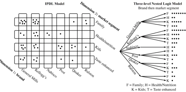
The IPDL model extends the nested logit model by allowing arbitrary, non-hierarchical grouping structures, i.e., any partitioning of the choice set in each dimension. Figure1illustrates the competing hierarchical and non-hierarchical grouping structures used for the empirical application in Section4. The freedom in defining grouping structures can be used to build inverse demand models that are similar in spirit to GEV models based on nesting, which have proved useful for demand estimation purposes (Train,2009, Chap. 4). For example, likeSmall

(1987) and Grigolon(2018), it is possible to define grouping structures that de-scribe markets where products are naturally ordered.

It is important to note that the parametrization of the IPDL model does not depend on the number of products, but instead on the number of segmentation dimensions. This is important because it implies that the IPDL model can handle markets involving very many products.

Estimation of the IPDL Model Combining Equations (6) and (7), the IPDL model boils down to a linear regression model of market shares on product char-acteristics and share terms

ln ( sjt s0t ) = x_jtβ− αpjt+ D ∑ d=1 µdln ( sjt ∑ k∈Gd(j)skt ) +ξjt, (8)

for all inside productsj = 1, . . . , J in each market t = 1, . . . , T .

Equation (8) has the same form as the logit and nested logit equations (see

Berry, 1994; Verboven, 1996a), except for the share terms. Under the standard assumption that product characteristics x_jtare exogenous, we must therefore find at leastD + 1 instruments: one instrument for price and for each of the D share terms.

Following the prevailing literature (see e.g.,Berry and Haile,2014;Reynaert and Verboven,2014; Armstrong,2016), both cost shifters and BLP instruments are good candidates for instruments. Cost shifters are appropriate instruments for prices but may not be appropriate for market shares because costs aﬀect the market shares only through prices. BLP instruments, which are functions of the characteristics of competing products and are commonly used to instrument prices, are also useful to instrument market shares. In theory, BLP instruments generally suﬃce for identification.11 However, in practice they may be weak and

(24)

then cost shifters are required.

FollowingVerboven(1996a) andBresnahan et al.(1997), the BLP instruments of the IPDL model include, for each dimension, the sums of characteristics for other products of the same group as well as the number of products within each group. These instruments reflect the degree of substitution and the closeness of products within a group and are therefore likely to aﬀect prices and within-group market shares. The same instruments can also be computed for products of the same type. Lastly, we can exploit the ownership structure of the market and compute the same instruments while distinguishing products of the same firms from products of competing firms. The idea is that prices, and thus market shares, depend on the ownership structure since multi-product firms set prices so as to maximize their total profits.

Links to Discrete Choice Models We show below that the IPDL model is con-sistent with a representative consumer model (RCM) with taste for variety and without income eﬀect. The RCM assumes the existence of a variety-seeking rep-resentative consumer who aggregates a population of consumers and chooses some quantity of every product, trading oﬀ variety against quality. It has been a workhorse of the international trade literature sinceDixit and Stiglitz(1977) and

Krugman (1979), and has also been used for demand estimation purposes (e.g.,

Pinkse and Slade,2004).

Specifically, as shown below, the IPDL model is consistent with a represen-tative consumer, endowed with income y, who chooses a vector st ∈ int(∆) of nonzero market shares in markett so as to maximize the utility

αy +∑ j∈J δjtsjt− ∑ j∈J sjtlnGj(st) , (9)

where Gj is defined by Equations (6) and (7), and where δj is a linear-in-price index. The second term in Equation (9) captures the net utility derived from the consumption of s_tin the absence of interaction among products and the last term expresses taste for variety.

As mentioned above, the IPDL model has the nested logit model, and thus the logit model, as special cases: the logit is obtained when product segmenta-tion does not matter, and the nested logit model is obtained when the grouping products increases.

(25)

structure is hierarchical. Thus some IDPL models are ARUM. On the other hand, as shown below and in contrast to any ARUM, some IDPL models allow comple-mentarity.12

Complementarity We use the standard definition of complementarity and sub-stitutability in the absence of income eﬀect (Samuelson, 1974), defining com-plementarity (resp., substitutability) as a negative (resp., positive) cross-price derivative of demand.13 Proposition4in AppendixA.3provides some properties of the IPDL model regarding the patterns of substitution, including the matrix of price derivatives of demand.

The IPDL model allows complementarity. To see this, suppose there are 3 inside products and one outside good. Inside products are grouped according to two dimensions: for the first dimension, product 1 is in one group, and products 2 and 3 are in a second group; for the second dimension, products 1 and 2 are in one group, and product 3 is in a second group. Products 1 and 3 are complements if the derivative of the demand for product 3 with respect to the price of product 1 is negative, that is, if14

(1− µ1− µ2) (s1+s2) (s2+s3)− µ1µ2s0s2> 0,

which simplifies to 4/3 > µ1µ2/(1− µ1− µ2) fors0= 1/2 and s1 =s2=s3 = 1/6. In

particular, products 1 and 3 are complements forµ1 =µ2 = 1/3, but are

substi-tutes forµ1=µ2= 0.45. With the representative consumer interpretation, the

pa-rameterµ0= 1−

∑D

d=1µd measures taste for variety over all products of the choice set and each parameterµd, ford ≥ 1, measures taste for variety across groups of products according to dimensiond: higher µd means that variety at the level of groups of products matters more, meaning that products in the same group in dimensiond are more similar (seeVerboven,1996b, for a similar interpretation of the nesting parameter of the nested logit model). Then complementarity in the IPDL model arises in a very intuitive way, due to taste for variety at the group level.

In Section 1 of the supplement, we provide some simulation results

investi-12_{It would be of interest to establish conditions under which the IDPL model is equivalent to}

an ARUM.

13_{This definition is diﬀerent from the one used by}_Gentzkow₍₂₀₀₇_{) in the context of an ARUM}

defined over bundles of products.

(26)

gating the patterns of substitution. We find that: (i) products of the same type are always substitutes, while products of diﬀerent types may be substitutes or complements; and (ii) closer products into the characteristics space used to form product types (i.e., higher values of µd and/or whether products belong to the same groups or not) have higher cross-price elasticities.

4 Empirical Illustration: Demand for Cereals

In this section, we illustrate the IPDL model by estimating the demand for ready-to-eat (RTE) cereals in Chicago in 1991 – 1992. This market has been studied extensively (see e.g.,Nevo,2001;Michel and Weiergraeber,2019) and it is known to exhibit product segmentation. We compare the results (in terms of elasticities and goodness-of-fit) from the IPDL model to those from two alternative nested logit models.

4.1 Data

Databases We use store-level scanner data from the Dominick’s Database, made available by the James M. Kilts Center, University of Chicago Booth School of Business. We supplement with data on the nutrient content of the RTE cere-als (sugar, energy, fiber, lipid, sodium, and protein) from the USDA Nutrient Database for Standard Reference and with monthly sugar prices from the web-site www.indexmundi.com.

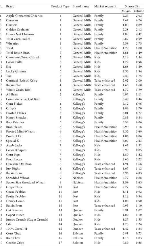
For our analysis, we use data from 83 Dominick’s stores and focus on the 50 largest products in terms of sales (e.g., Kellogg’s Special K), where a product is a cereal (e.g., Special K) associated to its brand (e.g., Kellogg’s). We define a market as a store-month pair. Prices of a serving (i.e., 35 grammes) and market shares are computed following Nevo (2001). See Appendix B for more details on the data.

Product Segmentation Based on the observations below, we consider two seg-mentation dimensions. The first dimension is brand, where the brands are Gen-eral Mills, Kellogg’s, Nabisco, Post, Quaker, and Ralston. The second dimension is market segment, where the market segments are family, kids, health/nutrition, and taste enhanced (see e.g.,Nevo,2001). These two dimensions are combined to form 17 product types among the 50 products.

(27)

Brands play an important role: Kellogg’s is the largest company and has large market shares in all market segments; and General Mills, the second largest com-pany, is especially popular in the family and kids segments. Taken together, Kel-logg’s and General Mills account for around 80 percent of the market. As regards market segments, the family and kids segments dominate and account for almost 70 percent of the market.

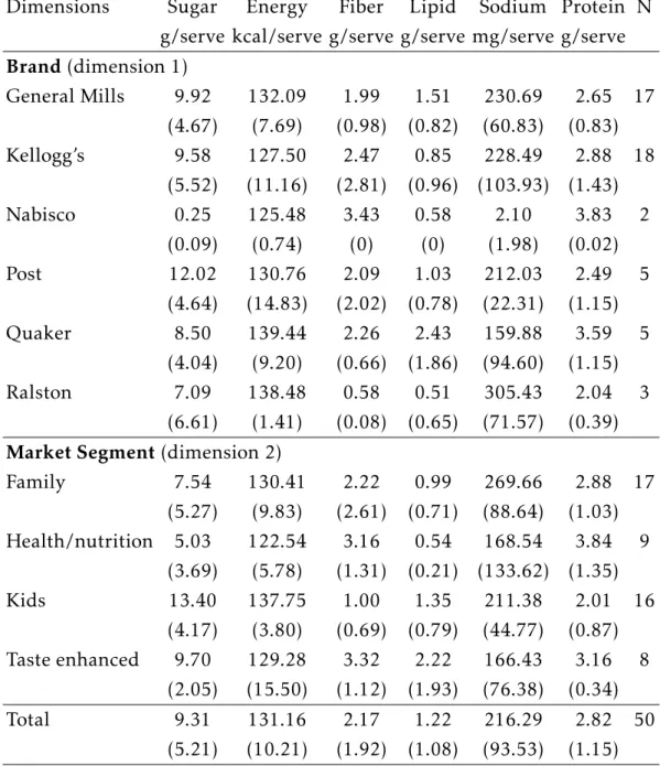
Table 1 shows the average nutrient content of the cereals grouped by brand and market segment. As expected, cereals for health/nutrition contain less sugar, more fiber, less lipid, and less sodium, and are less caloric. By contrast, cereals for kids contain more sugar and more calories. Moreover, Nabisco oﬀers cereals with less sugar and less calories, while Quaker and Ralston oﬀer cereals with more calories. The two dimensions therefore proxy, at least partially, for the nutrient content of the cereals.

Figure1illustrates the grouping structure of the IPDL model (left panel) and of the three-level nested logit model where products are grouped first by brand and then by market segment (right panel).

Figure 1: Product Segmentation on the Cereals Market

(28)

Table 1: Average by Market Segment and by Brand

Dimensions Sugar Energy Fiber Lipid Sodium Protein N

g/serve kcal/serve g/serve g/serve mg/serve g/serve Brand(dimension 1) General Mills 9.92 132.09 1.99 1.51 230.69 2.65 17 (4.67) (7.69) (0.98) (0.82) (60.83) (0.83) Kellogg’s 9.58 127.50 2.47 0.85 228.49 2.88 18 (5.52) (11.16) (2.81) (0.96) (103.93) (1.43) Nabisco 0.25 125.48 3.43 0.58 2.10 3.83 2 (0.09) (0.74) (0) (0) (1.98) (0.02) Post 12.02 130.76 2.09 1.03 212.03 2.49 5 (4.64) (14.83) (2.02) (0.78) (22.31) (1.15) Quaker 8.50 139.44 2.26 2.43 159.88 3.59 5 (4.04) (9.20) (0.66) (1.86) (94.60) (1.15) Ralston 7.09 138.48 0.58 0.51 305.43 2.04 3 (6.61) (1.41) (0.08) (0.65) (71.57) (0.39)

Market Segment(dimension 2)

Family 7.54 130.41 2.22 0.99 269.66 2.88 17 (5.27) (9.83) (2.61) (0.71) (88.64) (1.03) Health/nutrition 5.03 122.54 3.16 0.54 168.54 3.84 9 (3.69) (5.78) (1.31) (0.21) (133.62) (1.35) Kids 13.40 137.75 1.00 1.35 211.38 2.01 16 (4.17) (3.80) (0.69) (0.79) (44.77) (0.87) Taste enhanced 9.70 129.28 3.32 2.22 166.43 3.16 8 (2.05) (15.50) (1.12) (1.93) (76.38) (0.34) Total 9.31 131.16 2.17 1.22 216.29 2.82 50 (5.21) (10.21) (1.92) (1.08) (93.53) (1.15)

Notes: Standard deviations are reported in parentheses. Column "N" gives the number of

products by market segment and by brand. Averages and standard deviations are com-puted over products (without taking into account of their market shares).

4.2 Demand Estimation

Specification We estimate Equation (8), where xjt includes a constant, the nu-trients mentioned above and a dummy for promotion. FollowingBresnahan et al.

(29)

capture market-invariant observed and unobserved brand-specific and market segment-specific characteristics, respectively. The advantages provided by the two dimensions are therefore parametrized by the fixed eﬀects ξb andξs, which measure the extent to which belonging to a group shifts the demand for the prod-uct, as well as the parameters for groupsµ1 andµ2, which measure the extent to

which products within a group are protected from substitution from products in other groups along each dimension. Lastly, we include fixed eﬀects for month (ξm), and store (ξst), which capture monthly unobserved determinants of demand and time-invariant store characteristics, respectively.

The unobserved product characteristics terms are therefore given by ξjt=ξb+ξs+ξm+ξst+ ˜ξjt,

where ˜ξjt, the structural error that remain inξjt, capture the unobserved product characteristics varying across products and markets that are not included into the model (e.g., changes in shelf-space, positioning of the products among oth-ers), which aﬀect consumers utility and that consumers and firms (but not the modeller) observe so that they are likely to be correlated with prices and market shares.

Instruments We use two sets of instruments. First, as cost-based instruments, we form the price of the cereal’s sugar content of a serve (i.e., sugar content in a serve times the sugar monthly price), which we interact with brand fixed effects. Multiplying the price of sugar by the sugar content allows the instrument to vary by product; and interacting this with fixed effects allows the price of sugar to enter the production function of each firm differently.

Second, we form BLP instruments by using other products’ promotional ac-tivity in a given market, which varies both across stores for a given month and across months for a given store: for a given product, other products’ promo-tional activity should aﬀect consumers’ choices, and should thus be correlated with the price and market share of that product, but not with the error term.15

15_{We do not use functions of the nutrient content of the cereals as instruments since by}

con-struction of the data they are invariant across markets. We treat promotion as an exogenous variable since, at Dominick’s Finer Foods, the promotional calendar is known several weeks in advance of the weekly price decisions. One concern about the use of promotions to form instru-ments is that promotions could be advertised. If it was the case, this would mean that promotions are not exogenous and cannot be used as instruments. However, we do not observe advertising in the data, which is therefore part of the error term, and, in turn, we assume that promotions

(30)

Specifically, we use the number of other promoted products of rival firms and the number of other promoted products of the same firm, which we interact with brand name fixed eﬀects. We also use these numbers over products belonging to the same market segment, which we interact with market segment fixed eﬀects.

A potential problem is weak identification, which occurs when instruments are only weakly correlated with the endogenous variables. With multiple en-dogenous variables, the standard first-stage F-statistic is no longer appropriate to test for weak instruments. We therefore useSanderson and Windmeijer(2016)’s F-statistic to test whether each endogenous variable is weakly identified. In each estimated model, the F-statistics are far larger than 10, implying that we can be confident that instruments are not weak.

Parameter Estimates Table 2 presents the 2SLS demand estimates from the IPDL and the three-level nested logit models with groups for market segment on top (3NL1) and with groups for brand on top (3NL2), in columns (1), (2), and (3), respectively.

Consider first the results from the IPDL model. As expected, the estimated parameters on the negative of price (α) and on promotion (β) are significantly positive. The estimated parameters for groups have magnitude and sign that conform to the assumptions of the IPDL model,µ1≥ 0, µ2≥ 0 and 1 − µ1− µ2> 0;

no constraints were imposed on the parameters during the estimation. These estimates imply that there is product segmentation along both dimensions: for cereals of the same market segment, cereals of the same brand are closer substi-tutes than cereals of diﬀerent brands; and for cereals of the same brand, cereals within the same market segment are closer substitutes than cereals from diﬀerent market segments. Overall, cereals of the same type are closer substitutes.

We find that the brand reputation of the cereals confers a significant advan-tage to products from General Mills and Kellogg’s and that cereals for family have a significant advantage. In addition, we find thatµ1> µ2, which means that

the market segments confer more protection from substitution than brand repu-tation does (cereals of the same market segment are more protected from cereals from diﬀerent market segments than cereals of the same brand are from cereals of diﬀerent brands).

are not followed by advertising. SeeMichel and Weiergraeber(2019) who also use promotion to form instruments.

(31)

Table 2: Parameter Estimates of Demand

(1) (2) (3) IPDL 3NL1 3NL2 Price (−α) -1.83 (0.12) -2.91 (0.12) -4.10 (0.16) Promotion (β) 0.088 (0.003) 0.102 (0.003) 0.144 (0.004) Constant (β0) -0.697 (0.059) -0.379 (0.065) -0.195 (0.076) Nesting Parameters (µ) Market Segment/Group (µ1) 0.626 (0.009) 0.771 (0.008) 0.668 (0.011) Brand/Subgroup (µ2) 0.232 (0.009) 0.792 (0.007) 0.709 (0.010) FE Brands (ξb) Kellogg’s 0.024 (0.005) -0.056 (0.003) 0.104 (0.006) Nabisco -0.754 (0.024) -0.218 (0.011) -2.11 (0.02) Post -0.485 (0.014) -0.187 (0.008) -1.36 (0.01) Quaker -0.553 (0.015) -0.329 (0.014) -1.51 (0.01) Ralston -0.732 (0.025) -0.200 (0.011) -2.13 (0.02) FE Market Segments (ξs) Health/nutrition -0.672 (0.010) -0.855 (0.008) -0.069 (0.005) Kids -0.433 (0.009) -0.529 (0.009) 0.071 (0.005) Taste enhanced -0.710 (0.010) -0.903 (0.007) -0.088 (0.006) Observations 99281 99281 99281 RMSE 0.210 0.242 0.270

Notes: The dependent variable is ln(sjt/s0t). Regressions include fixed eﬀects (FE) for brands, market segments, months, and stores, as well as a constant, the nutrients (fiber, sugar, lipid, protein, energy, sodium) and a dummy for promotion. Robust standard errors are reported in parentheses. The values of the F-statistics in the first stages suggest that weak instruments are not a problem.

Model Selection and Robustness The estimates from the two nested logit mod-els satisfyµ2> µ1, which means that they are both consistent with random utility

maximization. Neither nested logit model can then be rejected on this criterion. The three estimated models are non-nested and have the same number of estimated parameters. Then the non-nested test ofRivers and Vuong(2002) can be used to determine which best fits the data. We find that the test strongly rejects both nested logit models in favor of the IPDL model.16

In many situations, consumers face choices involving a very large number

16_{The test statistic is given by}√_J_{× T}(_Q_ˆ 1− ˆQ2

)

/ ˆσ , where ˆQi is the value of the 2SLS objective function of model i evaluated at the demand estimates, and ˆσ2 is the estimated value of the variance of the diﬀerence between ˆQi’s. The null hypothesis is that the two non-nested models are asymptotically equivalent; the first (resp., second) alternative hypothesis is that model 1 (resp., model 2) is asymptotically better than model 2 (resp., model 1). This statistic must be evaluated against the standard normal distribution and we estimate ˆσ2 _{using 500 bootstrap replications.}

The test statistics of the two nested logit models (model 1) against the IDPL model (model 2) are 1509.77 and 3644.43, respectively.

(32)

of products (e.g., choice of a car or of a RTE cereal). We have estimated an al-ternative specification in which we define products as cereal-brand-store combi-nations, as it is commonly done in the vertical relationships literature (see e.g.,

Villas-Boas, 2007), and markets as months. The resulting specification, which has more than 4, 000 products, leads to very similar parameter estimates, thereby indicating that the results are fairly robust to the definitions of products and markets.

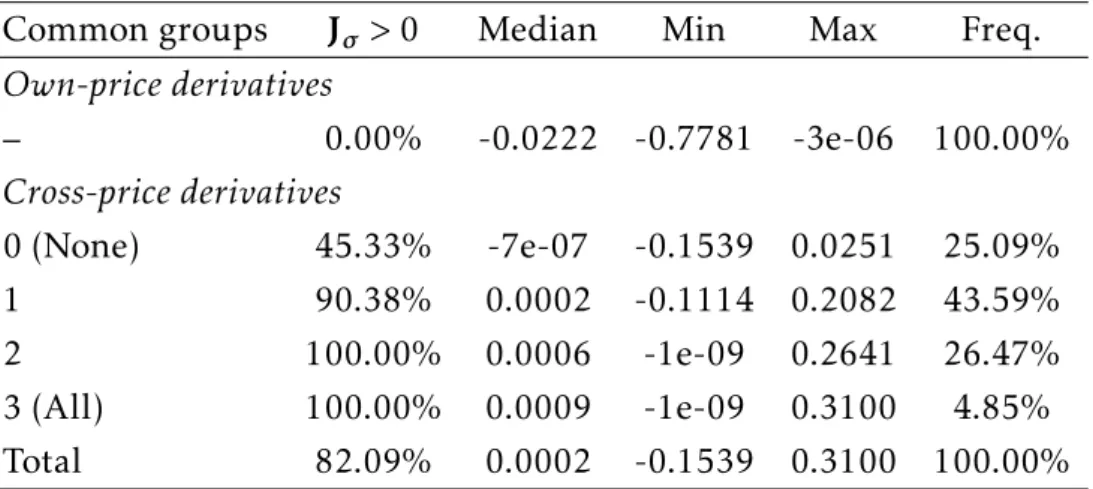
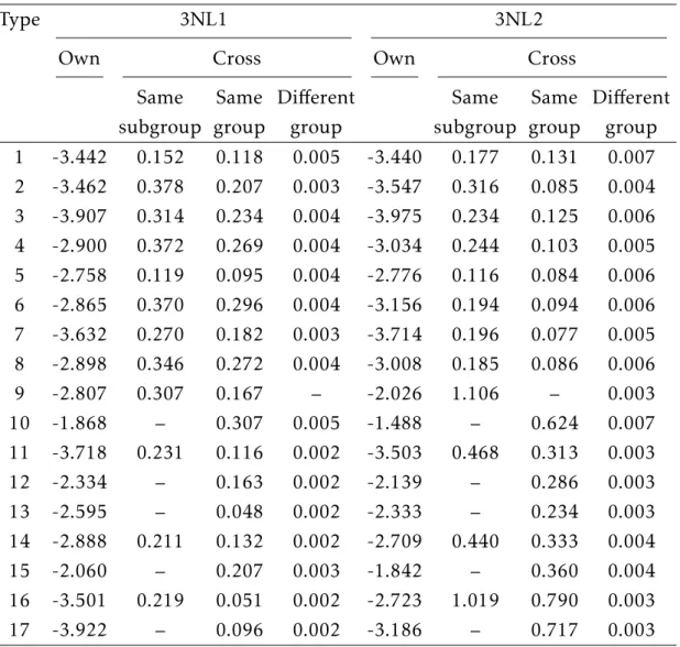
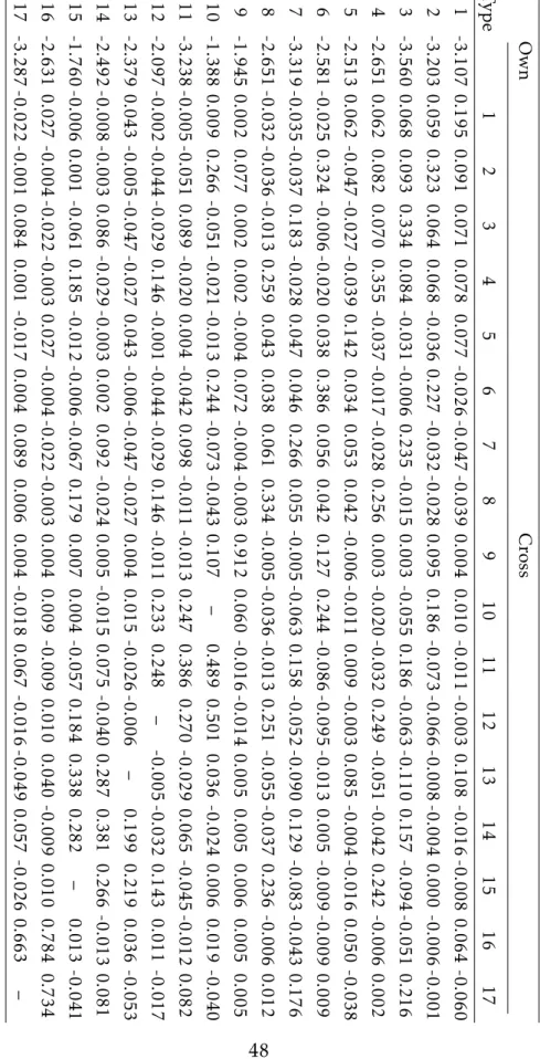
Substitution Patterns. Figure2presents the estimated density of the own- and cross-price elasticities of demands of the IPDL and the two nested logit models (see Section 3 of the supplement for the estimated own- and cross-price elastici-ties of demands, averaged across markets and product types).

The estimated own-price elasticities are in line with the literature (see e.g.,

Nevo,2001). On average, the estimated own-price elasticity of demands is−2.815 for the IPDL model,−3.187 for the 3NL1 model and −3.124 for the 3NL2 model. However, there is an important variation in price responsiveness across product types: for the IPDL model, own-price elasticities range from−3.560 for cereals for kids produced by General Mills to−1.388 for cereals for health/nutrition pro-duced by Post; for the 3NL1 model, they range from−3.923 for cereals for kids produced by Ralston to−1.868 for cereals for health/nutrition produced by Post; and for the 3NL2 model, they range from−3.975 for cereals for kids produced by General Mills to−1.488 for cereals for health/nutrition produced by Post.

Consider now the cross-price elasticities. Among the 50× 50 diﬀerent cross-price elasticities that the IPDL model yields, 49.5 percent (resp., 50.5 percent) are negative (resp., positive), meaning about one half of all pairs of cereals are com-plements. Note that the presence of complementarity is likely to reduce compe-tition in the cereals market compared to a case with no complementarity. Iaria and Wang(2019) also find that complementarity is pervasive in the RTE cereals market. Complementarity can arise for many reasons, including taste for variety and shopping costs.

Products of the same brand are always substitutes, which means that there is cannibalization effect; likewise, products from the same market segment are all substitutes. Products of different brands and of different market segments may or may not be complements.

(33)

Figure 2: Estimated Price Elasticities of Demands

5 The Generalized Inverse Logit Model

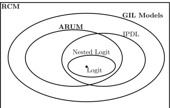
In this section, we introduce the Generalized Inverse Logit (GIL) class of models, which includes the IPDL model as a special case and hence also the logit and nested logit models. Proofs for this section are provided in AppendixA.4along with formal statements of the results. To ease exposition, we omit notation for parameters θ₂ and markett.

Definition 1. GIL models are inverse demands of the form (5), i.e.,

lnGj(s) = δj− c, j ∈ J , (10)

wherec∈ R is a market-specific constant and lnG =(lnG0, . . . , ln GJ )

is an inverse GIL demand.

An inverse GIL demand is a function ln G, where G : (0,∞)J+1 → (0,∞)J+1is homogeneous of degree one and where the Jacobian J_{ln G}(s) is positive definite and symmetric.

This definition immediately implies that the IDPL model is also a GIL model. Section 2 of the supplement provides a range of general methods for building inverse GIL demands along with illustrative examples that go beyond the IPDL

(34)

model, which is the focus of the paper. As stated in the following proposition, an inverse GIL demand is injective and hence invertible on its range.

Proposition 1. Let ln G be an inverse GIL demand. Then ln G is injective on int (∆).

We denote the inverse function as H = G−1. Inverting Equation (10) and us-ing that demands sum to one together with the homogeneity of G leads to the demand functions sj=σj(δ) = Hj ( eδ) ∑ k∈JHk(eδ) , j ∈ J . (11)

This expression generalizes the logit demands in a nontrivial way through the presence of the function H.

In addition, consider any vector of market shares s ∈ int(∆). Then, hold-ingδ0 = 0, the injectivity of the inverse GIL demand ensures that there exists a

unique vector of indexes δ =(0, δ1, . . . , δJ )

that rationalizes demand, i.e., s = σ (δ). Using that demands satisfy Roy’s identity ∂CS(eδ)/∂δj =σj(δ), it can easily be shown that the consumer surplus is

CS (δ) = ln   ∑ k∈J Hk ( eδ)   ,

up to an additive constant. Note that the consumer surplus is simply the loga-rithm of the denominator of the demands in Equation (11), just as in the case of the logit model.

Using that demands sum to one, we obtain that the market-specific constant is equal to the consumer surplusc = CS (δ), which combined with Equation (10), shows that GIL models satisfy

δj = lnGj(s) + CS (δ) , j ∈ J . (12)

Diﬀerentiating (12) with respect to δ, we find that the matrix of demand derivatives∂σj/∂δi is given by

Jσ(δ) = [Jln G(s)]−1− ss⊺, (13)

where s = σ (δ). Given the absence of income eﬀects, the matrix (13) is the Slutsky matrix. This is symmetric and positive semi-definite, which implies that GIL

(35)

demands are non-decreasing in their own indexδj,∂σj/∂δj ≥ 0.

The class of GIL models accommodates patterns that go beyond those of stan-dard ARUM. In particular, it allows for complementarity: this is for example the case of the IPDL model, which is a member of the class of GIL models. Our in-vertibility result in Proposition 1 therefore extends Berry (1994)’s invertibility result, which restricts the products to be strict substitutes. Proposition 1 also extendsBerry et al.(2013), who show invertibility for demands that satisfy their “connected substitutes” conditions, which rule out complementarity.17

6 Relationships between Models

This section puts the GIL and the IPDL models into perspective by showing how they relate to the representative consumer model (RCM) and to the additive ran-dom utility model (ARUM).

6.1 Representative Consumer Model

Consider a representative consumer facing the choice set of diﬀerentiated prod-ucts,J , and a homogeneous numéraire good, with demands for the diﬀerentiated products summing to one. Letpj andvj be the price and the quality of product j∈ J , respectively.

The price of the numéraire good is normalized to 1 and the representative consumer’s income y is suﬃciently high (y > maxj_∈Jpj) to guarantee that con-sumption of the numéraire good is positive.

In this subsection, we show that the inverse GIL demand ln G is consistent with a representative consumer who chooses a consumption vector s∈ ∆ of mar-ket shares of the diﬀerentiated product and a quantity z ≥ 0 of the numéraire

17_{The connected substitutes structure requires two conditions: (}_{i) products are weak gross}

substitutes, i.e., everything else equal, an increase inδi weakly decreases demandσj for all other products; and (ii) the “connected strict substitution” condition holds, i.e., there is suﬃcient strict

substitution between products to treat them in one demand system. In contrast to ours,Berry

et al. (2013)’s result does not require that demand σ is diﬀerentiable. Demand systems with

complementarity may be covered byBerry et al.(2013)’s result in cases where a suitable trans-formation of demand can be found such that the transformed demand satisfies their conditions. They provide no general result on how such a transformation could be found. Our result allows complementarity without requiring such a transformation to be found.

(36)

good, so as to maximize her direct utility αz +∑ j∈J vjsj− ∑ j∈J sjlnGj(s) (14)

subject to the budget constraint and the constraint that demands sum to one, ∑ j∈J pjsj+z≤ y and ∑ j∈J sj= 1, (15)

whereα > 0 is the marginal utility of income. The first two terms of the direct utility (14) describe the utility that the representative consumer derives from the consumption (s, z) of the diﬀerentiated products and the numéraire in the absence of interaction among them. The third term is a strictly concave function of s that expresses the representative consumer’s taste for variety (see Lemma4

in AppendixA.5).

Letδj =vj− αpj be the net utility that the consumer derives from consuming one unit of productj ∈ J . The utility maximization program (14)-(15) leads to first-order conditions for interior solution

lnGj(s) + c = δj, (16)

which are of the form of Equation (10) defining the inverse GIL demand.

We state this observation as a proposition and give a detailed proof in Ap-pendixA.5.

Proposition 2. The GIL model (16) is consistent with a representative consumer who maximizes utility (14) subject to constraints (15).

This proposition thus extends Anderson et al.(1988) andVerboven(1996b)’s results that the logit and the nested logit models are consistent with a utility maximizing representative consumer.

6.2 Additive Random Utility Model

We now turn to the Additive Random Utility Model. A population of consumers face the choice set of diﬀerentiated products, J , and associate a deterministic utility componentδj=vj− αpj to each productj ∈ J . Each individual consumer

Essais sur l'estimation structurelle de la demande

HAL Id: tel-02373983

https://tel.archives-ouvertes.fr/tel-02373983

Essais sur l’estimation structurelle de la demande

Julien Monardo

To cite this version:

Thèse

de

do

ctorat

NNT

:

2019SA

CLN042

Julien Monardo

Remerciements

Résumé de la thèse

Bibliographie

Contents

Notice

Chapter 1

The Inverse Product Di

ﬀerentiation

Logit Model

1

Introduction

2

Motivation

2.1

General Setting: the Role of Demand Inversion

2.2

Closed-Form and Linear-in-Parameters Inverse Demands

3

The Inverse Product Di

ﬀerentiation Logit (IPDL)

4

Empirical Illustration: Demand for Cereals

4.1

Data

4.2

Demand Estimation

5

The Generalized Inverse Logit Model

6

Relationships between Models

6.1

Representative Consumer Model

6.2

Additive Random Utility Model