COPYRIGHT NOTICE:

(1)

COPYRIGHT NOTICE:

Steven J. Miller and Ramin Takloo-Bighash:

An Invitation to Modern Number Theory

is published by Princeton University Press and copyrighted, © 2006, by Princeton

University Press. All rights reserved. No part of this book may be reproduced in any form

by any electronic or mechanical means (including photocopying, recording, or information

storage and retrieval) without permission in writing from the publisher, except for reading

and browsing via the World Wide Web. Users are not permitted to mount this file on any

network servers.

Follow links Class Use and other Permissions. For more information, send email to:

permissions@pupress.princeton.edu

(2)

Chapter Fifteen

From

Nuclear

Physics

to

L

Functions

In attempting to describe the energy levels of heavy nuclei ([Wig1, Wig3, Po, BFFMPW]), researchers were confronted with daunting calculations for a many bodied system with extremely complicated interaction forces. Unable to explicitly calculate the energy levels, physicists developed Random Matrix Theory to predict general properties of the systems. Surprisingly, similar behavior is seen in studying the zeros of Lfunctions!

In this chapter we give a brief introduction to classical Random Matrix Theory, Random Graphs and LFunctions. Our goal is to show how diverse systems ex hibit similar universal behaviors, and introduce the techniques used in the proofs. In some sense, this is a continuation of the Poissonian behavior investigations of Chapter 12. The survey below is meant to only show the broad brush strokes of this rich landscape; detailed proofs will follow in later chapters. We assume familiarity with the basic concepts of Lfunctions (Chapter 3), probability theory (Chapter 8) and linear algebra (a quick review of the needed background is provided in Appen dix B).

While we assume the reader has some familiarity with the basic concepts in physics for the historical introduction in §15.1, no knowledge of physics is required for the detailed expositions. After describing the physics problems, we describe several statistics of eigenvalues of sets of matrices. It turns out that the spacing properties of these eigenvalues is a good model for the spacings between energy levels of heavy nuclei and zeros of Lfunctions; exactly why this is so is still an open question. For those interested in learning more (as well as a review of recent developments), we conclude this chapter with a brief summary of the literature.

15.1 HISTORICAL INTRODUCTION

A central question in mathematical physics is the following: given some system with observables t1 ≤ t2 ≤ t3 ≤ . . . , describe how the ti are spaced. For example, we could take the ti to be the energy levels of a heavy nuclei, or the prime numbers, or zeros of Lfunctions, or eigenvalues of real symmetric or complex Hermitian matrices (or as in Chapter 12 the fractional parts {nkα} arranged in increasing order). If we completely understood the system, we would know exactly where all the ti are; in practice we try and go from knowledge of how the ti are spaced to knowledge of the underlying system.

(3)

15.1.1 Nuclear Physics

In classical mechanics it is possible to write down closed form solutions to the two body problem: given two points with masses m1 and m2 and initial velocities �v1 and �v2 and located at �r1 and �r2, describe how the system evolves in time given that gravity is the only force in play. The three body problem, however, deﬁes closed form solutions (though there are known solutions for special arrangements of special masses, three bodies in general position is still open; see [Wh] for more details). From physical grounds we know of course a solution must exist; how ever, for our solar system we cannot analyze the solution well enough to determine whether or not billions of years from now Pluto will escape from the sun’s inﬂu ence! In some sense this is similar to the problems with the formula for counting primes in Exercise 2.3.18.

Imagine how much harder the problems are in understanding the behavior of heavy nuclei. Uranium, for instance, has over 200 protons and neutrons in its nu cleus, each subject to and contributing to complex forces. If the nucleus were com pletely understood, one would know the energy levels of the nucleus. Physicists were able to gain some insights into the nuclear structure by shooting highenergy neutrons into the nucleus, and analyzing the results; however, a complete under standing of the nucleus was, and still is, lacking. Later, when we study zeros of Lfunctions from number theory, we will ﬁnd analogues of highenergy neutrons!

One powerful formulation of physics is through inﬁnite dimensional linear alge bra. The fundamental equation for a system becomes

Hψn = Enψn, (15.1)

where H is an operator (called the Hamiltonian) whose entries depend on the physical system and the ψn are the energy eigenfunctions with eigenvalues En. Unfortunately for nuclear physics, H is too complicated to write down and solve; however, a powerful analogy with Statistical Mechanics leads to great insights.

15.1.2 Statistical Mechanics

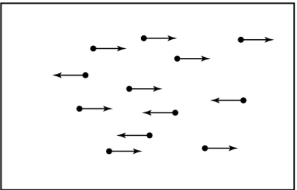
For simplicity consider N particles in a box where the particles can only move left or right and each particle’s speed is v; see Figure 15.1.

If we want to calculate the pressure on the left wall, we need to know how many particles strike the wall in an infinitesimal time. Thus we need to know how many particles are close to the left wall and moving towards it. Without going into all of the physics (see for example [Re]), we can get a rough idea of what is happen ing. The complexity, the enormous number of configurations of positions of the molecules, actually helps us. For each configuration we can calculate the pressure due to that configuration. We then average over all configurations, and hope that a generic configuration is, in some sense, close to the system average.

Wigner’s great insight for nuclear physics was that similar tools could yield use ful predictions for heavy nuclei. He modeled the nuclear systems as follows: in stead of the inﬁnite dimensional operator H whose entries are given by the physical laws, he considered collections of N × N matrices where the entries were inde pendently chosen from some probability distribution p. The eigenvalues of these

(4)

361

FROMNUCLEARPHYSICSTO LFUNCTIONS

Figure 15.1 Molecules in a box

matrices correspond to the energy levels of the physical system. Depending on physical symmetries, we consider different collections of matrices (real symmet ric, complex Hermitian). For any given ﬁnite matrix we can calculate statistics of the eigenvalues. We then average over all such matrices, and look at the limits as . The main result is that the behavior of the eigenvalues of an arbitrary N → ∞

matrix is often well approximated by the behavior obtained by averaging over all matrices, and this is a good model for the energy levels of heavy nuclei. This

is reminiscent of the Central Limit Theorem (§8.4). For example, if we average over all sequences of tossing a fair coin 2N times, we obtain N heads, and most sequences of 2N tosses will have approximately N heads.

Exercise 15.1.1. Consider 2N identical, indistinguishable particles, which are in the left (resp., right) half of the box with probability 1 ₂. What is the expected number

3 4

of particles in each half? What is the probability that one half has more than (2N )

3 4

particles than the other half? As (2N ) � N , most systems will have similar behavior although of course some will not. The point is that a typical system will be close to the system average.

Exercise 15.1.2. Consider 4N identical, indistinguishable particles, which are in the left (resp., right) half of the box with probability 1 ₂; each particle is moving left (resp., right) with probability 1 ₂. Thus there are four possibilities for each particle, and each of the 44N conﬁgurations of the 4N particles is equally likely. What is the

3

expected number of particles in each possibility (leftleft, leftright, rightleft, right right)? What is the probability that one possibility has more than (4N ) particles4

than the others? As (4N )3 4 � N , most systems will have similar behavior.

15.1.3 Random Matrix Ensembles

The ﬁrst collection of matrices we study are N × N real symmetric matrices, with the entries independently chosen from a ﬁxed probability distribution p on R. Given

(5)

such a matrix A, _⎛

a11 a12 a13 · · · a1N ⎞ A = ⎜ ⎜ ⎜ ⎝ a21 . . . a22 . . . a23 . . . · · · . . _. a2N . . . ⎟ ⎟ ⎟ ⎠ = A T _(15.2) aN 1 aN 2 aN 3 · · · aN N (so aij = aji), the probability density of observing A is

Prob(A)dA = � p(aij )daij . (15.3) 1≤i≤j≤N

We may interpret this as giving the probability of observing a real symmetric matrix where the probability of the ijth entry lying in [aij , aij + daij ] is p(aij )daij . More explicitly,

Prob(A : aij ∈ [αij , βij ]) =

� � βij

p(aij )daij . (15.4) 1≤i≤j≤N αij

Example 15.1.3. For a 2 × 2 real symmetric matrix we would have

A =

�

a11 a12 �

, Prob(A) = p(a11)p(a12)p(a22)da11da12da22. (15.5) a12 a22

An N × N real symmetric matrix is determined by specifying N (N +1) ₂ entries: there are N entries on the main diagonal, and N 2 − N offdiagonal entries (for these entries, only half are needed, as the other half are determined by symmetry). We say such a matrix has N (N ₂+1) degrees of freedom. Because p is a probability

density, it integrates to 1. Thus

�

Prob(A)dA = � � ∞

p(aij )daij = 1; (15.6) 1≤i≤j≤N aij =−∞

this corresponds to the fact that we must choose some matrix.

For convergence reasons we often assume that the moments of p are ﬁnite. We mostly study p(x) satisfying

p(x) ≥ 0 � ∞ p(x)dx = 1 � ∞ −∞ k x p(x)dx < ∞. (15.7) | | −∞

The last condition ensures that the probability distribution is not too spread out (i.e., there is not too much probability near inﬁnity). Many times we normalize p so that the mean (ﬁrst moment) is 0 and the variance (second moment if the mean is zero) is 1.

Exercise 15.1.4. For the kth _moment�

R xk p(x)dx to exist, we require

�

R |x|k p(x)dx < ∞; if this does not hold, the value of the integral could depend on how we ap

proach inﬁnity. Find a probability function p(x) and an integer k such that

� A � 2A

k k

lim x p(x)dx = 0 but lim x p(x)dx = ∞. (15.8)

(6)

363

Exercise 15.1.5. Let p be a probability density such that all of its moments exist. If

p is an even (resp., odd) function, show all the odd (resp., even) moments vanish.

Exercise 15.1.6. Let p be a continuous probability density on R. Show there exist constants a, b such that q(x) = a · p(ax + b) has mean 0 and variance 1. Thus in some sense the third and the fourth moments are the ﬁrst “free” moments as the above transformation is equivalent to translating and rescaling the initial scale.

Exercise 15.1.7. It is not necessary to choose each entry from the same probability distribution. Let the ijth entry be chosen from a probability distribution pij . What

is the probability density of observing A? Show this also integrates to 1.

Deﬁnition 15.1.8 (Ensembles). A collection of matrices, along with a probability density describing how likely it is to observe a given matrix, is called an ensemble of matrices (or a random matrix ensemble).

Example 15.1.9. Consider the ensemble of 2 × 2 real symmetric matrices A where

x y for a matrix A = � y z �, 2 � 3 _{if x}2 _{+ y}2 _{+ z ≤ 1} p(A) = 4π _(15.9) 0 otherwise.

Note the entries are not independent. We can parametrize these matrices by using spherical coordinates. For a sphere of radius r we have

x = x(r, θ, φ) = r cos(θ) sin(φ) y = y(r, θ, φ) = r sin(θ) sin(φ)

z = z(r, θ, φ) = r cos(φ), (15.10)

where θ ∈ [0, 2π] is the azimuthal angle, φ ∈ [0, π] is the polar angle and the volume of the sphere is 4 πr3 _.

3

In this introduction we conﬁne ourselves to real symmetric matrices, although many other ensembles of matrices are important. Complex Hermitian matrices (the generalization of real symmetric matrices) also play a fundamental role in the theory. Both of these types of matrices have a very important property: their

eigenvalues are real; this is what allows us to ask questions such as how are the

spacings between eigenvalues distributed.

In constructing our real symmetric matrices, we have not said much about the probability density p. In Chapter 17 we show for that some physical problems, additional assumptions about the physical systems force p to be a Gaussian. For many of the statistics we investigate, it is either known or conjectured that the answers should be independent of the speciﬁc choice of p; however, in this method of constructing random matrix ensembles, there is often no unique choice of p. Thus, for this method, there is no unique answer to what it means to choose a matrix at random.

Remark 15.1.10 (Advanced). We would be remiss if we did not mention another

notion of randomness, which leads to a more natural method of choosing a ma trix at random. Let U (N ) be the space of N × N unitary matrices, and consider

(7)

� �

its compact subgroups (for example, the N × N orthogonal matrices). There is a natural (canonical) measure, called the Haar measure, attached to each of these compact groups, and we can use this measure to choose matrices at random. Fur ther, the eigenvalues of unitary matrices have modulus 1. They can be written as eiθj _{, with the θ}

j real. We again obtain a sequence of real numbers, and can again ask many questions about spacings and distributions. This is the notion of random matrix ensemble which has proven the most useful for number theory.

Exercise 15.1.11. Prove the eigenvalues of real symmetric and complex Hermitian matrices are real.

Exercise 15.1.12. How many degrees of freedom does a complex Hermitian matrix have?

15.2 EIGENVALUE PRELIMINARIES 15.2.1 Eigenvalue Trace Formula

Our main tool to investigate the eigenvalues of matrices will be the Eigenvalue Trace Formula. Recall the trace of a matrix is the sum of its diagonal entries:

Trace(A) = a11 +· · · + aN N . (15.11) We will also need the trace of powers of matrices. For example, a 2 × 2 matrices

a11 a12 _(15.12)

A = _a21 _a22 , we have

Trace(A2_{) = a}_11a11_{+ a}_12a21_{+ a}_12a21_{+ a}_22a22₌ 2 � 2 � aij aji. N � i=1 j=1 (15.13) In general we have

Theorem 15.2.1. Let A be an N × N matrix. Then

N � Trace(Ak₎₌ _ai _(15.14) k−1 ik aik i1 . ai1 i2 ai2 i3 · · · · · · i1 =1 ik =1

For small values of k, instead of using i1, i2, i3, . . . we often use i, j, k, . . . . For example, Trace(A3) = �_i�_j�_kaij ajkaki.

Exercise 15.2.2. Show (15.13) is consistent with Theorem 15.2.1. Exercise 15.2.3. Prove Theorem 15.2.1.

Theorem 15.2.4 (Eigenvalue Trace Formula). For any nonnegative integer k, if A is an N × N matrix with eigenvalues λi(A), then

N

�

Trace(Ak_{) =} _λi_(A)k _. _(15.15) i=1

(8)

365

The importance of this formula is that it relates the eigenvalues of a matrix (which is what we want to study) to the entries of A (which is what we choose at random). The importance of this formula cannot be understated – it is what makes the whole subject possible.

Sketch of the proof. The case k = 1 follows from looking at the characteristic poly

nomial det(A − λI) = 0. For higher k, note any matrix A can be conjugated to an upper triangular matrix: U −1AU = T where T is upper triangular and U is uni tary. The eigenvalues of A equal those of T and are given by the diagonal entries of T . Further the eigenvalues of Ak equal those of T k . If λi(A) and λi(Ak ) are the eigenvalues of A and Ak , note λi(Ak ) = λi(A)k . The claim now follows by applying the k = 1 result to the matrix Ak:

Trace(Ak _{) =} N � λi(Ak _{) =} N � λi(A)k _. _(15.16) i=1 i=1

Exercise 15.2.5. Prove all the claims used in the proof of the Eigenvalue Trace For mula. If A is real symmetric, one can use the diagonalizability of A. To show any matrix can be triangularized, start with every matrix has at least one eigenvalue eigenvector pair. Letting −v1 →be the eigenvector, using GramSchmidt one can ﬁnd an orthonormal basis. Let these be the columns of U1, which will be a unitary

matrix. Continue by induction.

15.2.2 Normalizations

Before we can begin to study fine properties of the eigenvalues, we first need to figure out what is the correct scale to use in our investigations. For example, the celebrated Prime Number Theorem (see Theorem 13.2.10 for an exact statement of the error term) states that π(x), the number of primes less than x, satisfies

x

π(x) = + lower order terms. (15.17)

log x

Remark 15.2.6. If we do not specify exactly how much smaller the error terms

are, we do not need the full strength of the Prime Number Theorem; Chebyshev’s arguments (Theorem 2.3.9) are sufﬁcient to get the order of magnitude of the scale.

x

The average spacing between primes less than x is about _{x/ log x}= log x, which

tends to infinity as x → ∞. Asking for primes that differ by 2 is a very hard question: as x → ∞, this becomes insignificant on the “natural” scale. Instead, a more natural question is to inquire how often two primes are twice the average spacing apart. This is similar to our investigations in Chapter 12 where we needed to find the correct scale.

If we ﬁx a probability density p, how do we expect the sizes of the eigenvalues λi(A) to depend on N as we vary A? A good estimate falls out immediately from

the Eigenvalue Trace Formula; this formula will be exploited numerous times in the arguments below, and is essential for all investigations in the subject.

(9)

We give a heuristic for the eigenvalues of our N ×N ensembles of matrices being roughly of size √N . Fix a matrix A whose entries aij are randomly and indepen dently chosen from a ﬁxed probability distribution p with mean 0 and variance 1. By Theorem 15.2.1, for A = AT we have that

Trace(A2) = N � N � aij aji = N � N � a 2 ij . (15.18) i=1 j=1 i=1 j=1 2

From our assumptions on p, we expect each a_ijto be of size 1. By the Central Limit Theorem (Theorem 8.4.1) or Chebyshev’s Theorem (Exercise 8.1.55), we expect with high probability

N � N � 2 a_ij∼ N2 _·_1, _(15.19) i=1 j=1 2

with an error of size √N2 = N (as each a_ijis approximately of size 1 and there are N2 of them, with high probability their sum should be approximately of size N2_{). Thus} N � λi(A)2 _{∼ N}2 _, _(15.20) i=1 which yields N · Ave(λi(A)2) ∼ N2 . (15.21) For heuristic purposes we shall pass the square root through to get

|Ave(λi(A))| ∼ √N . (15.22) In general the square root of an average need not be the same as the average of the square root; however, our purpose here is merely to give a heuristic as to the correct scale. Later in our investigations we shall see that √N is the correct normalization. Thus it is natural to guess that the correct scale to study the eigenvalues of an N × N real symmetric matrix is c√N , where c is some constant independent of N . This yields normalized eigenvalues �λ1(A) = λi (A) _{; choosing c = 2 leads to}

c√N

clean formulas. One could of course normalize the eigenvalues by f (N ), with f an undetermined function, and see which choices of f give good results; eventually one would ﬁnd f (N ) = c√N .

Exercise 15.2.7. Consider real N × N matrices with entries independently chosen from a probability distribution with mean 0 and variance 1. How large do you expect the average eigenvalue to be?

Exercise 15.2.8. Use Chebyshev’s Theorem (Exercise 8.1.55) to bound the proba

2

bility that |�_i�_ja_ij− N2_|_{≥ N log N . Conclude that with high probability that}

(10)

FROMNUCLEARPHYSICSTO LFUNCTIONS 367

15.2.3 Eigenvalue Distribution

We quickly review the theory of point masses and induced probability distributions (see §11.2.2 and §12.5). Let δx0 represent a unit point mass at x0. We deﬁne its action on functions by

� _∞

δx0 (f ) := f (x)δ(x − x0)dx = f (x0). (15.23) −∞

δx0 , called the Dirac delta functional at x0, is similar to our approximations to the identity. There is ﬁnite mass (its integral is 1), the density is 0 outside x0 and inﬁnite at x0. As its argument is a function and not a complex number, δx0 is a

functional and not a function. To each A, we attach a probability measure (the eigenvalue probability distribution):

1 N µA,N (x)dx = � δ � x − λi(A) � dx. (15.24) N _i=1 2√N 1 At each normalized eigenvalue λi (A) _{we have placed a mass of weight}

N ; there 2√N

are N masses, thus we have a probability distribution. If p(x) is a probability distribution then � _ab p(x)dx is the probability of observing a value in [a, b]. For us,

� _b

µA,N (x)dx is the percentage of normalized eigenvalues in [a, b]:

a

� _b _{#{i :}λi (A)

2√N ∈ [a, b]

µA,N (x)dx = } . (15.25)

a N

We can calculate the moments of µA,N (x).

Deﬁnition 15.2.9. Let E[xk ]A denote the kth moment of µA,N (x). We often denote

this MN,k(A).

The following corollary of the Eigenvalue Trace formula is the starting point of many of our investigations; we see in Remark 15.3.15 why it is so useful.

)

Lemma 15.2.10. MN,k (A) = Trace(A

k . k

2k _N2 +1

Proof. As Trace(Ak ) = �_iλi(A)k _{we have} k

�

k

MN,k (A) = E[x ]A = x µA,N (x)dx N 1 �� x − λi(A) � = x k_δ 2√N dx N _i=1 R N 1 � λi(A)k = N (2√N )k i=1 Trace(Ak ₎ = . (15.26) 2k_Nk 2 +1 2

Exercise 15.2.11. Let A be an N × N real symmetric matrix with a| ij |≤ B. In

terms of B, N and k bound Trace(A| k) and M| N,k (A). How large can maxi |λi(A)|

(11)

15.3 SEMICIRCLE LAW 15.3.1 Statement

A natural question to ask concerning the eigenvalues of a matrix is: What percent

age of the normalized eigenvalues lie in an interval [a, b]? Let µA,N (x) be the eigenvalue probability distribution. For a given A, the answer is

� b

µA,N (x)dx. (15.27)

a

How does the above behave as we vary A? We have the following startling result, which is almost independent of the underlying probability density p we used to choose the entries of A:

Theorem 15.3.1 (SemiCircle Law). Consider the ensemble of N × N real sym metric matrices with entries independently chosen from a ﬁxed probability density

p(x) with mean 0, variance 1, and ﬁnite higher moments. As N → ∞, for almost

all A, µA,N (x) converges to the semicircle density 2 √

1 − x2_. π

Thus the percentage of normalized eigenvalues of A in [a, b] [−1, 1] for a typical A as N → ∞ is ⊂ � _b 2 � 1 − x2_dx. _(15.28) π a

Later in §15.3.4 we discuss what happens if the higher moments are inﬁnite.

15.3.2 Moment Problem

We brieﬂy describe a needed result from Probability Theory: the solution to the Moment Problem. See page 110 of [Du] for details; see [ShTa] for a connection between the moment problem and continued fractions!

Let k be a nonnegative integer; below we always assume m0 = 1. We are inter ested in when numbers mk determine a unique probability distribution P whose kth moment is mk . If the mk do not grow too rapidly, there is at most one continuous probability density with these moments (see [Bi, CaBe, Fe]). A sufﬁcient condition

mj tj

is Carleman’s Condition that �∞_j=1m_2j−1/2j = ∞. Another is that �∞_{j=1 j!} has a positive radius of convergence. This implies the moment generating function (see Exercise 15.3.2) exists in an interval and the distribution is uniquely determined.

Exercise 15.3.2 (Nonuniqueness of moments). For x ∈ [0, ∞), consider

√ 2 1 πxe −(log x)2 _/2 f1(x) = f2(x) = f1(x) [1 + sin(2π log x)] . (15.29) r

Show that for r ∈ N, the rth moment of f1 and f2 is e 2 _/2

. The reason for the nonuniqueness of moments is that the moment generating function

� _∞

Mf (t) = e txf (x)dx (15.30) −∞

(12)

�

FROMNUCLEARPHYSICSTO LFUNCTIONS 369

does not converge in a neighborhood of the origin. See [CaBe], Chapter 2. See also Exercise A.2.7.

For us the numbers mk arise from averaging the moments MN,k (A) of the µA,N (x)’s and taking the limit as N → ∞. Let

MN,k = MN,k(A)Prob(A)dA, mk = lim MN,k . (15.31)

A N →∞

For each N the moments MN,k yield a probability distribution PN , and limN →∞ MN,k = mk . If the mk grow sufﬁciently slowly, there is a unique continuous probability density P with kth _{moment m}

k. It is reasonable to posit that as for each k, limN →∞ MN,k = mk , then “most” µA,N (x) converge (in some sense) to the probability density P (x).

N

Remark 15.3.3 (Warning). For each N , consider N numbers {an,N }n=1 deﬁned by an,N = 1 if n is even and −1 if N is odd. For N even, note the average of the an,N ’s is 0, but each a| n,N | = 1; thus, no element is close to the system average. Therefore, it is not always the case that a typical element is close to the system average. What is needed in this case is to consider the variance of the moments (see Exercise 15.3.5).

Remark 15.3.4. While it is not true that every sequence of numbers mk that grow sufﬁciently slowly determines a continuous probability density (see Exercise 15.3.8), as our mk arise from limits of moments of probability distributions, we do obtain a unique limiting probability density. This is similar to determining when a Taylor series converges to a unique function. See also Exercise A.2.7.

N

Exercise 15.3.5. Let {bn,N }n=1 be a sequence with mean µ(N ) = 1

�N bn,N

N n=1

1

and variance σ2(N ) = _N �N _n=1|bn,N − µ(N )2 . Assume that as N → ∞,

µ(N ) → µ and σ2_{(N ) → 0. Prove for any � >} |

0 as N → ∞ for a ﬁxed N at most � percent of bn,N are not within � of µ. Therefore, if the mean of a sequence

converges and we have control over the variance, then we have control over the limiting behavior of most elements.

In this text we content ourselves with calculating the average moments mk =

limN →∞

�

MN,k(A)dA. In many cases we derive simple expressions for the

A

probability density P with moments mk; however, we do not discuss the probability arguments needed to show that as N → ∞, a “typical” matrix A has µA,n(x) close to P . The interested reader should see [CB, HM] for an application to moment arguments in random matrix theory.

Some care is needed in formulating what it means for two probability distribu tions to be close. For us, µA,N (x) is the sum of N Dirac delta functionals of mass

1

N . Note |P (x) − µA,N (x) can be large for individual x. For example, if P (x) is| the semicircle distribution, then P (x) − µ| A,N (x) will be of size 1 for almost all |

[−1, 1]. We need to deﬁne what it means for two probability distributions to

x ∈ be close.

One natural measure is the KolmogoroffSmirnov discrepancy. For a probability distribution f (x) its Cumulative Distribution Function Cf (x) is deﬁned to be the

(13)

�

probability of [−∞, x]:

x

Cf (x) = f (x)dx. (15.32) −∞

If our distribution is continuous, note this is the same as the probability of [−∞, x); however, for distributions arising from Dirac delta functionals like our µA,N (x), there will be ﬁnite, nonzero jumps in the cumulative distribution function at the normalized eigenvalues. For example, for µA,N (x) we have

1 CµA,N (x) = _N � 1, (15.33) λi (A) _{< x} 2√N 1

which jumps by at least _N at each normalized eigenvalue. For two probability distributions f and g we deﬁne the KolmogoroffSmirnov discrepency of f and g to be sup_x|Cf (x) − Cg (x) . Note as N → ∞ each normalized eigenvalue| contributes a smaller percentage of the total probability. Using the Kolmogoroff Smirnov discrepancy for when two probability distributions are close, one can show that as N → ∞ “most” µA,N (x) are close to P .

Remark 15.3.6. It is not true that all matrices A yield µA,N (x) that are close to P ; for example, consider multiples of the identity matrix. All the normalized eigenvalues are the same, and these real symmetric matrices will clearly not have µA,N (x) close to P (x). Of course, as N → ∞ the probability of A being close to

a multiple of the identity matrix is zero.

Exercise 15.3.7. Fix a probability distribution p, and consider N × N real sym metric matrices with entries independently chosen from p. What is the probability that a matrix in this ensemble has all entries within � of a multiple of the N × N identity matrix? What happens as N → ∞ for ﬁxed �? How does the answer depend on p?

Exercise 15.3.8. Let mk be the kth moment of a probability density P . Show

2 m0

m2m0 − m1 ≥ 0. Note this can be interpreted as

� � m1 m1 � � ≥ 0. Thus, if m2 2

m2m0 − m1 < 0, the mk cannot be the moments of a probability distribution.

Find a similar relation involving m0, m1, m2, m3 and m4 and a determinant. See

[Chr] and the references therein for more details, as well as [ShTa, Si] (where the determinant condition is connected to continued fraction expansions!).

Exercise 15.3.9. If p(x) = 0 for x > R, show the kth _{moment satisﬁes m}

k ≤ Rk _{. Hence lim}_{j→∞ m}1/2j < ∞ | . |

Therefore, if a probability distribution has

2j

limj→∞ m 1/2j _2j = ∞, then for any R there is a positive probability of observing

|x| > R. Alternatively, we say such p has unbounded support. Not surprisingly,

the Gaussian moments (see Exercise 15.3.10) grow sufﬁciently rapidly so that the Gaussian has unbounded support.

Exercise 15.3.10 (Moments of the Gaussian). Calculate the moments of the Gaussian

g(x) = √1 2π e

−x 2 _/2

. Prove the odd moments vanish and the even moments are

(14)

� | � � � � 371

ways to match 2k objects in pairs. Show the moments grow sufﬁciently slowly to determine a unique continuous probability density.

Exercise 15.3.11. Consider two probability distributions f and g on [0, 1] where

f (x) = 1 for all x and g(x) = 1 for x �∈ Q and 0 otherwise. Note both f and g assign the same probability to any [a, b] with b = a. Show sup_x∈[0,1]f (x) − g(x) = 1 but the KolmogoroffSmirnov discrepancy is zero. Thus looking at the |

pointwise difference could incorrectly cause us to conclude that f and g are very different.

Exercise 15.3.12. Do there exist two probability distributions that have a large KolmogoroffSmirnov discrepancy but are close pointwise?

15.3.3 Idea of the Proof of the SemiCircle Law

We give a glimpse of the proof of the SemiCircle Law below; a more detailed sketch will be provided in Chapter 16. We use Moment Method from §15.3.2.

k

For each µA,N (x), we calculate its kthmoment, MN,k (A) = E[x ]A. Let MN,k be the average of MN,k (A) over all A. We must show as N → ∞, MN,k converges to the kth moment of the semicircle. We content ourselves with just the second moment below, and save the rest for §16.1. By Lemma 15.2.10,

MN,k (A)Prob(A)dA MN,2 = A 1 22_N2 2 +1 _A Trace(A2_)Prob(A)dA. _(15.34) =

We use Theorem 15.2.1 to expand Trace(A2) and ﬁnd 1 �N �N ₂

ij Prob(A)dA. (15.35)

MN,2 = a

22_N2

A i=1 j=1 We now expand Prob(A)dA by (15.3):

MN,2

1 � ∞ � ∞ �N �N ₂

ij · p(a11)da11 · · · p(aN N )daN N

= a

22_N2 · · ·

a11 =−∞ aN N =−∞ _{i=1 j=1} 1 �N �N � ∞ � ∞

2

ij · p(a11)da11 · · · p(aN N )daN N ;

= a

22_N2 · · ·

i=1 j=1 a11 =−∞ aN N =−∞

(15.36) we may interchange the summations and the integrations as there are ﬁnitely many sums. For each of the N 2 pairs (i, j), we have terms like

� _∞ 2 ij p(aij )daij · � _∞ p(akl)dakl. (15.37) a aij =−∞ (k,l)=(ij) � akl =−∞ k≤l

The above equals 1. The ﬁrst factor is 1 because it is the variance of aij , which was assumed to be 1. The second factor is a product of integrals where each integral

(15)

is 1 (because p is a probability density). As there are N 2 summands in (15.36), we

1 1

ﬁnd MN,2 = ₄(so limN →∞ MN,2 = ₄), which is the second moment of the semicircle.

Exercise 15.3.13. Show the second moment of the semicircle is 1 ₄.

Exercise 15.3.14. Calculate the third and fourth moments, and compare them to those of the semicircle.

Remark 15.3.15 (Important). Two features of the above proof are worth highlight

ing, as they appear again and again below. First, note that we want to answer a question about the eigenvalues of A; however, our notion of randomness gives us information on the entries of A. The key to converting information on the entries to knowledge about the eigenvalues is having some type of Trace Formula, like Theorem 15.2.4.

The second point is the Trace Formula would be useless, merely converting us from one hard problem to another, if we did not have a good Averaging Formula, some way to average over all random A. In this problem, the averaging is easy because of how we deﬁned randomness.

Remark 15.3.16. While the higher moments of p are not needed for calculating

MN,2 = E[x2_{], their ﬁniteness comes into play when we study higher moments.}

15.3.4 Examples of the SemiCircle Law

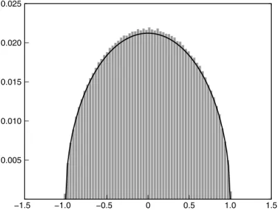
First we look at the density of eigenvalues when p is the standard Gaussian, p(x) = √1

2π e −x 2 _/2

. In Figure 15.2 we calculate the density of eigenvalues for 500 such matrices (400 × 400), and note a great agreement with the semicircle.

What about a density where the higher moments are inﬁnite? Consider the Cauchy distribution,

1

(15.38) p(x) =

π(1 + x2₎.

The behavior is clearly not semicircular (see Figure 15.3). The eigenvalues are unbounded; for graphing purposes, we have put all eigenvalues greater than 300 in the last bin, and less than 300 in the ﬁrst bin.

Exercise 15.3.17. Prove the Cauchy distribution is a probability distribution by showing it integrates to 1. While the distribution is symmetric, one cannot say the mean is 0, as the integral � | |x p(x)dx = ∞. Regardless, show the second moment is inﬁnite.

15.3.5 Summary

Note the universal behavior: though the proof is not given here, the SemiCircle Law holds for all mean zero, ﬁnite moment distributions. The independence of the behavior on the exact nature of the underlying probability density p is a common feature of Random Matrix Theory statements, as is the fact that as N → ∞ most

(16)

373

−1.5 −1.0 −0.5 0 0.5 1.0 1.5 0.005 0.010 0.015 0.020 0.025

Figure 15.2 Distribution of eigenvalues: 500 Gaussian matrices (400 × 400)

−300 −200 −100 0 100 200 300 500 1000 1500 2000 2500

(17)

A yield µA,N (x) that are close (in the sense of the KolmogoroffSmirnov discrep

ancy) to P (where P is determined by the limit of the average of the moments MN,k(A)). For more on the SemiCircle Law, see [Bai, BK].

15.4 ADJACENT NEIGHBOR SPACINGS 15.4.1 GOE Distribution

The SemiCircle Law (when the conditions are met) tells us about the density of eigenvalues. We now ask a more reﬁned question:

Question 15.4.1. How are the spacings between adjacent eigenvalues distributed?

For example, let us write the eigenvalues of A in increasing order; as A is real symmetric, the eigenvalues will be real:

(15.39) λ1(A) ≤ λ2(A) ≤ · · · ≤ λN (A).

The spacings between adjacent eigenvalues are the N − 1 numbers

λ2(A) − λ1(A), λ3(A) − λ2(A), . . . , λN (A) − λN −1(A). (15.40) As before (see Chapter 12), it is more natural to study the spacings between adja cent normalized eigenvalues; thus, we have

λ2(A) λ1(A) λN (A) λN −1(A)

, . . . ,

2√N − 2√N 2√N − 2√N . (15.41)

Similar to the probability distribution µA,N (x), we can form another probability distribution νA,N (s) to measure spacings between adjacent normalized eigenval ues. Deﬁnition 15.4.2. N 1 � δ �

s − λi(A) − λi−1(A)

�

νA,N (s)ds =

N − 1 _i=2 2√N ds. (15.42) Based on experimental evidence and some heuristical arguments, it was con jectured that as N → ∞, the limiting behavior of νA,N (s) is independent of the probability density p used in randomly choosing the N × N matrices A.

Conjecture 15.4.3 (GOE Conjecture:). As N → ∞, νA,N (s) approaches a uni

versal distribution that is independent of p.

Remark 15.4.4. GOE stands for Gaussian Orthogonal Ensemble; the conjecture is

known if p is (basically) a Gaussian. We explain the nomenclature in Chapter 17.

Remark 15.4.5 (Advanced). The universal distribution is π_{4 dt}2 d2 Ψ 2 , where Ψ(t) is (up to constants) the Fredholm determinant of the operator f � t K ∗ f with

1 � sin(ξ−η) ₊sin(ξ+η) �

→ _−t

kernel K = _2π _ξ+η . This distribution is well approximated by πs 2 � pW (s) = π _{s exp}� ξ− 4 η . 2 −

(18)

375

πs 2

Exercise 15.4.6. Prove pW (s) = π s exp

�

4

�

is a probability distribution with

2 −

mean 1. What is its variance?

We study the case of N = 2 and p a Gaussian in detail in Chapter 17.

Exercise(hr) 15.4.7 (Wigner’s surmise). In 1957 Wigner conjectured that as N

∞ the spacing between adjacent normalized eigenvalues is given by

→ π � πs2 �

pW (s) =

2 s exp − 4 . (15.43) He was led to this formula from the following assumptions:

Given an eigenvalue at x, the probability that another one lies s units to its

•

right is proportional to s.

Given an eigenvalue at x and I1, I2, I3, . . . any disjoint intervals to the right

•

of x, then the events of observing an eigenvalue in Ij are independent for all j.

The mean spacing between consecutive eigenvalues is 1.

•

Show these assumptions imply (15.43).

15.4.2 Numerical Evidence

We provide some numerical support for the GOE Conjecture. In all the experiments below, we consider a large number of N × N matrices, where for each matrix we look at a small (small relative to N ) number of eigenvalues in the bulk of the

eigenvalue spectrum (eigenvalues near 0), not near the edge (for the semicircle,

eigenvalues near ±1). We do not look at all the eigenvalues, as the average spac ing changes over such a large range, nor do we consider the interesting case of the largest or smallest eigenvalues. We study a region where the average spacing is ap proximately constant, and as we are in the middle of the eigenvalue spectrum, there are no edge effects. These edge effects lead to fascinating questions (for random graphs, the distribution of eigenvalues near the edge is related to constructing good networks to rapidly transmit information; see for example [DSV, Sar]).

First we consider 5000 300 × 300 matrices with entries independently chosen from the uniform distribution on [−1, 1] (see Figure 15.4). Notice that even with N as low as 300, we are seeing a good ﬁt between conjecture and experiment.

What if we take p to be the Cauchy distribution? In this case, the second moment of p is inﬁnite, and the alluded to argument for semicircle behavior is not applica ble. Simulations showed the density of eigenvalues did not follow the SemiCircle Law, which does not contradict the theory as the conditions of the theorem were not met. What about the spacings between adjacent normalized eigenvalues of real symmetric matrices, with the entries drawn from the Cauchy distribution?

We study 5000 100 × 100 and then 5000 300 × 300 Cauchy matrices (see Figures 15.5 and 15.6. We note good agreement with the conjecture, and as N increases the ﬁt improves.

(19)

0 0.5 1.0 1.5 2.0 2.5 3.0 3.5 4.0 4.5 5.0 0.5 1.0 1.5 x 104 2.0 2.5 3.0 3.5

Figure 15.4 The local spacings of the central threeﬁfths of the eigenvalues of 5000 matrices (300 × 300) whose entries are drawn from the Uniform distribution on [−1, 1]

0 0.5 1.0 1.5 2.0 2.5 3.0 3.5 4.0 4.5 5.0 2,000 4,000 6,000 8,000 10,000 12,000

Figure 15.5 The local spacings of the central threeﬁfths of the eigenvalues of 5000 matrices (100 × 100) whose entries are drawn from the Cauchy distribution

(20)

377

0 0.5 1.0 1.5 2.0 2.5 3.0 3.5 4.0 4.5 5.0 0.5 1.0 1.5 x 104 2.0 2.5 3.0 3.5

Figure 15.6 The local spacings of the central threeﬁfths of the eigenvalues of 5000 matrices (300 × 300) whose entries are drawn from the Cauchy distribution

We give one last example. Instead of using continuous probability distribution, we investigate a discrete case. Consider the Poisson Distribution:

λn

p(n) = e−λ . (15.44) n!

We investigate 5000 300 × 300 such matrices, ﬁrst with λ = 5, and then with λ = 20, noting again excellent agreement with the GOE Conjecture (see Figures 15.7 and 15.8):

15.5 THIN SUBFAMILIES

Before moving on to connections with number theory, we mention some very im portant subsets of real symmetric matrices. The subsets will be large enough so that there are averaging formulas at our disposal, but thin enough so that sometimes we see new behavior. Similar phenomena will resurface when we study zeros of Dirichlet Lfunctions.

As motivation, consider as our initial set all even integers. Let N2(x) denote the x

number of even integers at most x. We see N2(x) ∼ ₂, and the spacing between adjacent integers is 2. If we look at normalized even integers, we would have yi = 2

2 i , and now the spacing between adjacent normalized even integers is 1. Now consider the subset of even squares. If N2(x) is the number of even squares at most x, then N2(x) ∼

√ x

. For even squares of size x, say x = (2m)2, the next 2

(21)

0 0.5 1.0 1.5 2.0 2.5 3.0 3.5 4.0 4.5 5.0 0.5 1.0 1.5 x 104 2.0 2.5 3.0 3.5

Figure 15.7 The local spacings of the central threeﬁfths of the eigenvalues of 5000 matrices (300 × 300) whose entries are drawn from the Poisson distribution (λ = 5)

0 0.5 1.0 1.5 2.0 2.5 3.0 3.5 4.0 4.5 5.0 0.5 1.0 1.5 x 104 2.0 2.5 3.0 3.5

Figure 15.8 The local spacings of the central threeﬁfths of the eigenvalues of 5000 matrices (300 × 300) whose entries are drawn from the Poisson distribution (λ = 20)

(22)

379

1

2

3

4

Figure 15.9 A typical graph

even square is at (2m + 2)2 = x + 8m + 4. Note the spacing between adjacent

even squares is about 8m ∼ 4√x for m large.

Exercise 15.5.1. By appropriately normalizing the even squares, show we obtain a new sequence with a similar distribution of spacings between adjacent elements as in the case of normalized even integers. Explicitly, look at the spacings between

N consecutive even squares with each square of size x and N � x.

Remark 15.5.2. A far more interesting example concerns prime numbers. For the

first set, consider all prime numbers. For the subset, fix an integer m and consider all prime numbers p such that p + 2m is also prime; if m = 1 we say p and p + 2 are a twin prime pair. It is unknown if there are infinitely many elements in the second set for any m, though there are conjectural formulas (using the techniques of Chapter 13). It is fascinating to compare these two sets; for example, what is the spacing distribution between adjacent (normalized) primes look like, and is that the same for normalized twin prime pairs? See Research Project 12.9.5.

15.5.1 Random Graphs: Theory

A graph G is a collection of points (the vertices V ) and lines connecting pairs of points (the edges E). While it is possible to have an edge from a vertex to itself (called a selfloop), we study the subset of graphs where this does not occur. We will allow multiple edges to connect the same two vertices (if there are no multiple edges, the graph is simple). The degree of a vertex is the number of edges leaving (or arriving at) that vertex. A graph is dregular if every vertex has exactly d edges leaving (or arriving).

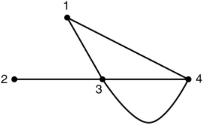
For example, consider the graph in Figure 15.9: The degrees of vertices are 2, 1, 4 and 3, and vertices 3 and 4 are connected with two edges.

To each graph with N vertices we can associate an N ×N real symmetric matrix, called the adjacency matrix, as follows: First, label the vertices of the graph from

1 to N (see Exercise 15.5.3). Let aij be the number of edges from vertex i to vertex j. For the graph above, we have

A = ⎛ ⎜ ⎜ ⎝ 0 0 1 1 0 0 1 0 1 1 0 2 1 0 2 0 ⎞ ⎟ ⎟ ⎠ . (15.45)

(23)

For each N , consider the space of all dregular graphs. To each graph G we associate its adjacency matrix A(G). We can build the eigenvalue probability dis tributions (see §15.2.3) as before. We can investigate the density of the eigenvalues and spacings between adjacent eigenvalues. We are no longer choosing the matrix elements at random; once we have chosen a graph, the entries are determined. Thus we have a more combinatorial type of averaging to perform: we average over all graphs, not over matrix elements. Even though these matrices are all real symmet ric and hence a subset of the earlier ensembles, the probability density for these matrices are very different, and lead to different behavior (see also Remark 16.2.13 and §7.10).

One application of knowledge of eigenvalues of graphs is to network theory. For example, let the vertices of a graph represent various computers. We can transmit information between any two vertices that are connected by an edge. We desire a well connected graph so that we can transmit information rapidly through the sys tem. One solution, of course, is to connect all the vertices and obtain the complete

graph. In general, there is a cost for each edge; if there are N vertices in a simple

graph, there are N (N ₂−1) possible edges; thus the complete graph quickly becomes very expensive. For N vertices, dregular graphs have only dN ₂ edges; now the cost is linear in the number of vertices. The distribution of eigenvalues (actually, the second largest eigenvalue) of such graphs provide information on how well con nected it is. For more information, as well as speciﬁc constructions of such well connected graphs, see [DSV, Sar].

Exercise 15.5.3. For a graph with N vertices, show there are N ! ways to label the vertices. Each labeling gives rise to an adjacency matrix. While a graph could potentially have N ! different adjacency matrices, show all adjacency matrices have the same eigenvalues, and therefore the same eigenvalue probability distribution.

Remark 15.5.4. Fundamental quantities should not depend on presentation. Exer

cise 15.5.3 shows that the eigenvalues of a graph do not depend on how we label the graph. This is similar to the eigenvalues of an operator T : Cn _→Cn _{do not} depend on the basis used to represent T . Of course, the eigenvectors will depend on the basis.

Exercise 15.5.5. If a graph has N labeled vertices and E labeled edges, how many ways are there to place the E edges so that each edge connects two distinct vertices? What if the edges are not labeled?

Exercise 15.5.6 (Bipartite graphs). A graph is bipartite if the vertices V can be split into two distinct sets, A1 and A2, such that no vertices in an Ai are connected

by an edge. We can construct a dregular bipartite graph with #A1 = #A2 = N .

Let A1 be vertices 1, . . . , N and A2 be vertices N + 1, . . . , 2N . Let σ1, . . . , σd

be permutations of {1, . . . , N }. For each σj and i ∈ {1, . . . , N }, connect vertex i ∈ A1 to vertex N + σj (i) ∈ A2. Prove this graph is bipartite and dregular. If d = 3, what is the probability (as N → ∞) that two vertices have two or more

(24)

381

Remark 15.5.7. Exercise 15.5.6 provides a method for sampling the space of bi

partite dregular graphs, but does this construction sample the space uniformly (i.e., is every dregular bipartite graph equally likely to be chosen by this method)? Fur ther, is the behavior of eigenvalues of dregular bipartite graphs the same as the behavior of eigenvalues of dregular graphs? See [Bol], pages 50–57 for methods to sample spaces of graphs uniformly.

Exercise 15.5.8. The coloring number of a graph is the minimum number of colors needed so that no two vertices connected by an edge are colored the same. What is the coloring number for the complete graph on N ? For a bipartite graph with N vertices in each set?

Consider now the following graphs. For any integer N let GN be the graph with

vertices the integers 2, 3, . . . , N , and two vertices are joined if and only if they have a common divisor greater than 1. Prove the coloring number of G10000 is at least

13. Give good upper and lower bounds as functions of N for the coloring number of GN .

15.5.2 Random Graphs: Results

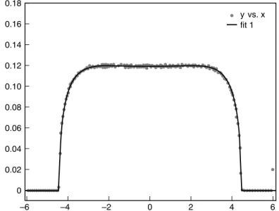
The ﬁrst result, due to McKay [McK], is that while the density of states is not the semicircle there is a universal density for each d.

Theorem 15.5.9 (McKay’s Law). Consider the ensemble of all dregular graphs with N vertices. As N → ∞, for almost all such graphs G, µA(G),N (x) converges

to Kesten’s measure d f (x) = � 2π(d2 _−x � 4(d − 1) − x2 _, _x 2 ₎ | | ≤ 2 √ d − 1 (15.46) 0 otherwise.

Exercise 15.5.10. Show that as d → ∞, by changing the scale of x, Kesten’s measure converges to the semicircle distribution.

Below (Figures 15.10 and 15.11) we see excellent agreement between theory and experiment for d = 3 and 6; the data is taken from [QS2].

The idea of the proof is that locally almost all of the graphs almost always look like trees (connected graphs with no loops), and for trees it is easy to calculate the eigenvalues. One then does a careful bookkeeping. Thus, this subfamily is thin enough so that a new, universal answer arises. Even though all of these adjacency matrices are real symmetric, it is a very thin subset. It is because it is such a thin subset that we are able to see new behavior.

Exercise 15.5.11. Show a general real symmetric matrix has N (N +1) ₂ independent entries, while a dregular graph’s adjacency matrix has dN ₂ nonzero entries.

What about spacings between normalized eigenvalues? Figure 15.12 shows that, surprisingly, the result does appear to be the same as that from all real symmetric matrices. See [JMRR] for more details.

(25)

–3 –2 –1 0 1 2 3 0.05 0.10 0.15 0.20 0.25 0.30 0.35 0 y vs. _x fit 1

Figure 15.10 Comparison between theory (solid line) and experiment (dots) for 1000 eigen values of 3regular graphs (120 bins in the histogram)

–6 –4 –2 0 2 4 6 0.06 0.08 0.10 0.12 0.14 0.16 y vs. _x fit 1 0.18 0.04 0.02 0

Figure 15.11 Comparison between theory (solid line) and experiment (dots) for 1000 eigen values of 6regular graphs (240 bins in the histogram)

(26)

383

0.5 1.0 1.5 2.0 2.5 3.0 0 0.1 0.2 0.3 0.4 0.5 0.6 0.7

Figure 15.12 3regular, 2000 vertices (graph courtesy of [JMRR])

15.6 NUMBER THEORY

We assume the reader is familiar with the material and notation from Chapter 3. For us an Lfunction is given by a Dirichlet series (which converges if �s is sufﬁ ciently large), has an Euler product, and the coefﬁcients have arithmetic meaning:

∞ an(f )

L(s, f ) = � = � Lp(p−s, f )−1 , �s > s0. (15.47) ns

n=1 p

The Generalized Riemann Hypothesis asserts that all nontrivial zeros have �s =

1 1

2 ; i.e., they are on the critical line �s = 2and can be written as 1 2 + iγ, γ ∈ R. The simplest example is ζ(s), where an(ζ) = 1 for all n; in Chapter 3 we saw how information about the distribution of zeros of ζ(s) yielded insights into the be havior of primes. The next example we considered were Dirichlet Lfunctions, the Lfunctions from Dirichlet characters χ of some conductor m. Here an(χ) = χ(n),

and these functions were useful in studying primes in arithmetic progressions. For a fixed m, there are φ(m) Dirichlet Lfunctions modulo m. This provides our first example of a family of Lfunctions. We will not rigorously define a family, but content ourselves with saying a family of Lfunctions is a collection of “similar” Lfunctions.

The following examples will be considered families: (1) all Dirichlet Lfunctions with conductor m; (2) all Dirichlet Lfunctions with conductor m ∈ [N, 2N ]; (3) all Dirichlet Lfunctions arising from quadratic characters with prime conductor p ∈ [N, 2N ]. In each of the cases, each Lfunction has the same conductor, similar functional equations, and so on. It is not unreasonable to think they might share other properties.

(27)

2

Another example comes from elliptic curves. We commented in §4.2.2 that given a cubic equation y2 = x3 + Af x + Bf , if ap(f ) = p − Np (where Np is the number of solutions to y2 ≡ x3 _{+ A}_{f x + Bf}_{mod p), we can construct an Lfunction using} the ap(f )’s. We construct a family as follows. Let A(T ), B(T ) be polynomials with integer coefﬁcients in T . For each t ∈ Z, we get an elliptic curve Et (given by y = x3 + A(t)x + B(t)), and can construct an Lfunction L(s, Et). We can consider the family where t ∈ [N, 2N ].

Remark 15.6.1. Why are we considering “restricted” families, for example Dirich

let Lfunctions with a fixed conductor m, or m ∈ [N, 2N ], or elliptic curves with t ∈ [N, 2N ]? The reason is similar to our random matrix ensembles: we do not consider infinite dimensional matrices: we study N × N matrices, and take the limit as N → ∞. Similarly in number theory, it is easier to study finite sets, and then investigate the limiting behavior.

1

Assuming the zeros all lie on the line �s = ₂, similar to the case of real sym metric or complex Hermitian matrices, we can study spacings between zeros. We now describe some results about the distribution of zeros of Lfunctions. Two clas sical ensembles of random matrices play a central role: the Gaussian Orthogonal Ensemble GOE (resp., Gaussian Unitary Ensemble GUE), the space of real sym metric (complex Hermitian) matrices where the entries are chosen independently from Gaussians; see Chapter 17. It was observed that the spacings of energy levels of heavy nuclei are in excellent agreement with those of eigenvalues of real sym metric matrices; thus, the GOE became a common model for the energy levels. In §15.6.1 we see there is excellent agreement between the spacings of normalized zeros of Lfunctions and those of eigenvalues of complex Hermitian matrices; this led to the belief that the GUE is a good model for these zeros.

15.6.1 nLevel Correlations

In an amazing set of computations starting at the 1020th zero, Odlyzko [Od1, Od2] observed phenomenal agreement between the spacings between adjacent normal ized zeros of ζ(s) and spacings between adjacent normalized eigenvalues of com plex Hermitian matrices. Speciﬁcally, consider the set of N × N random Hermitian matrices with entries chosen from the Gaussian distribution (the GUE). As N → ∞ the limiting distribution of spacings between adjacent eigenvalues is indistinguish able from what Odlyzko observed in zeros of ζ(s)!

His work was inspired by Montgomery [Mon2], who showed that for suitable test functions the pair correlation of the normalized zeros of ζ(s) agree with that of normalized eigenvalues of complex Hermitian matrices. Let {αj } be an increasing sequence of real numbers, B ⊂ Rn−1 a compact box. Deﬁne the nlevel correla

tion by # ��αj1 − αj2 , . . . , αjn−1 − αjn � ∈ B, ji ≤ N ; ji = jk � lim � . (15.48) N N →∞

For example, the 2level (or pair) correlation provides information on how often two normalized zeros (not necessarily adjacent zeros) have a difference in a given

(28)

385

interval. One can show that if all the nlevel correlations could be computed, then we would know the spacings between adjacent zeros.

We can regard the box B as a product of n−1 characteristic functions of intervals (or binary indicator variables). Let

�

1 if x ∈ [ai, bi],

Iai ,bi (x) = (15.49) 0 otherwise.

We can represent the condition x ∈ B by IB (x) =

�_n

Ia_i,bi (xi). Instead of

i=1

using a box B and its function IB , it is more convenient to use an inﬁnitely differ entiable test function (see [RS] for details). In addition to the pair correlation and the numerics on adjacent spacings, Hejhal [Hej] showed for suitable test functions the 3level (or triple) correlation for ζ(s) agrees with that of complex Hermitian matrices, and RudnickSarnak [RS] proved (again for suitable test functions) that the nlevel correlations of any “nice” Lfunction agree with those of complex Her mitian matrices.

The above work leads to the GUE conjecture: in the limit (as one looks at zeros with larger and larger imaginary part, or N × N matrices with larger and larger N ), the spacing between zeros of Lfunctions is the same as that between eigenvalues of complex Hermitian matrices. In other words, the GUE is a good model of zeros of Lfunctions.

Even if true, however, the above cannot be the complete story.

Exercise 15.6.2. Assume that the imaginary parts of the zeros of ζ(s) are un bounded. Show that if one removes any ﬁnite set of zeros, the nlevel correlations are unchanged. Thus this statistic is insensitive to ﬁnitely many zeros.

The above exercise shows that the nlevel correlations are not sufﬁcient to cap ture all of number theory. For many Lfunctions, there is reason to believe that there is different behavior near the central point s = 1 ₂ (the center of the critical strip) than higher up. For example, the Birch and SwinnertonDyer conjecture (see §4.2.2) says that if E(Q) (the group of rational solutions for an elliptic curve E; see §4.2.1) has rank r, then there are r zeros at the central point, and we might expect different behavior if there are more zeros.

Katz and Sarnak [KS1, KS2] proved that the nlevel correlations of complex Hermitian matrices are also equal to the nlevel correlations of the classical com

pact groups: unitary matrices (and its subgroups of symplectic and orthogonal

matrices) with respect to Haar measure. Haar measure is the analogue of ﬁxing a probability distribution p and choosing the entries of our matrices randomly from p; it should be thought of as specifying how we “randomly” chose a matrix from these groups. As a unitary matrix U satisﬁes U∗U = I (where U∗ _{is the complex} conjugate transpose of U ), we see each entry of U is at most 1 in absolute value, which shows unitary matrices are a compact group. A similar argument shows the set of orthogonal matrices Q such that QT Q = I is compact.

What this means is that many different ensembles of matrices have the same nlevel correlations – there is not one unique ensemble with these values. This led to a new statistic which is different for different ensembles, and allows us to “determine” which matrix ensemble the zeros follow.

COPYRIGHT NOTICE: