Lire
la
première partie
265
Annex A. GNSS signals
In this annex, a general view of the structure of a GNSS signal is presented and the architecture of a GNSS receiver is described. Nevertheless, before presenting the general structure of a GNSS signal, the minimum information data needed to provide positioning service is explained.
A.1. Minimum information data
The main fields needed to provide positioning service can be reduced to two different types of information. On one hand, the receiver-satellite distance; on the other hand, the satellite position with respect to Earth [MACABIAU and JULIEN, 2009] [SPILKER and ASHBYa, 1996].
A.1.1. Pseudo-range measurement
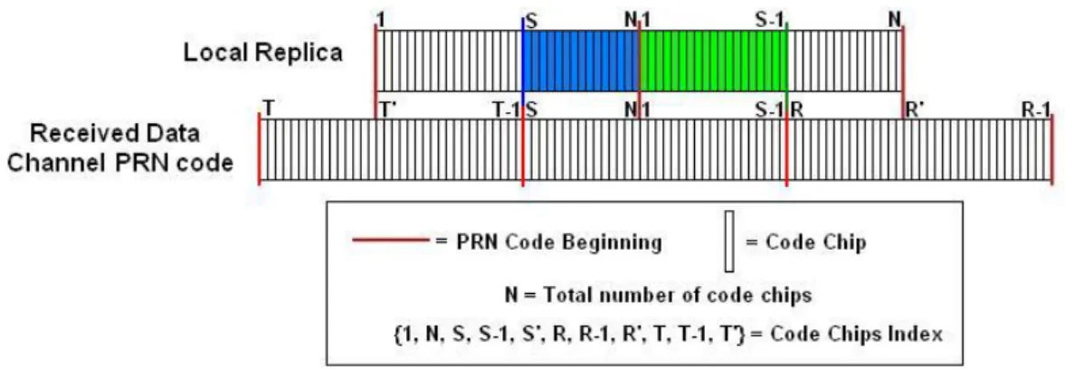
A receiver needs to know the distance between a GNSS satellite and itself. This distance is calculated from the signal propagation time and it is called pseudo-range [SPILKER and ASHBYb, 1996]. The pseudo-range is measured as the time offset between the signal received from the satellite at the antenna output and a local replica of this same signal generated by the receiver taking into account that the receiver ideally knows the time at which the satellite emitted the signal. The pseudo-range is the sum of the distance and the satellite-receiver clock offset. This means that the satellite-receiver has to take into account this lack of synchronization in order to correctly estimate the distance between the satellite and the receiver and thus in order to correctly estimate the user position. More specifically, the receiver and the satellite clocks should be both synchronized with the common GNSS general time but the reality is that neither of them is. Moreover, the lack of synchronization of each clock is processed differently due to the very different clock qualities.
In fact, the clock quality is much higher for a satellite clock, which is an atomic clock, than for a receiver clock which is not very accurate [SPILKER and ASHBYa, 1996]. Therefore, whereas the satellite clock bias is modeled as en error over the pseudo-range measurement, the receiver clock bias is so important and particular for each individual clock that the receiver is obliged to estimate the clock bias in order to remove its influence over the pseudo-range measurement.
The receiver cannot estimate its position with only one satellite pseudo-range, which means that the pseudo-range of several satellites should be used. Indeed, assuming a perfect synchronization between the satellites and the receiver clocks, with one satellite pseudo-range, the user position range is a sphere centered at the satellite position. With two satellite pseudo-ranges, the user position range is reduced to the common points (intersection) of the two satellite spheres, a circumference. And with three satellites pseudo-ranges, the user position range is reduced to only two points. Nevertheless, one of the two points is directly discarded because it is not placed on the Earth surface. Therefore, with three satellites a user should be able to estimate its position [SPILKER and ASHBYb, 1996]. See Figure A-1 for a graphical explanation.
266
Figure A-1: Receiver positioning scheme with 3 received satellite pseudo-ranges
When assuming that the satellites and the receiver clocks are not synchronized, in order to obtain a 3-Dimensional user position, the receiver needs to measure 4 satellite pseudo-ranges; three satellites for the three user position components (x, y, z) and one for the user clock bias [SPILKER and ASHBYb, 1996].
Moreover, some additional information is required in order to correct pseudo-range measurement errors, such as the influence of the ionosphere, troposphere, etc and the previously commented satellite clock bias [MACABIAU and JULIEN, 2009].
A.1.2. Satellite ephemeris data
The receiver has to know the absolute position of the satellites, because, as it can be observed from Figure A-1, the estimated user position depends on the satellites position. Therefore, in order to obtain an absolute position instead of a relative one, the user has to know what the absolute positions of the satellites are.
A.1.3. Mathematical model of the estimation of the user position
Once the minimum information date needed to estimate a user position has been explained, the mathematical model which allows the user position estimation is given. This mathematical model relates the corrected pseudo-ranges measurements to the receiver position components and to the receiver clock bias [MACABIAU and JULIEN, 2009]:
) ( ) ( ) ( ) ( ) ( ) ( ) ( ) ( ) ( 2 2 2 2 2 2 2 2 2 2 2 1 2 1 2 1 2 1 1 k b k t c z z y y x x k P k b k t c z z y y x x k P k b k t c z z y y x x k P n u n n n n u u (A-1) Where: Pi(k): pseudo-range measurement of satellite i after applying the best corrections
(x, y, z): user coordinates
267
c: velocity of light in vacuum
Δtu: user clock bias
bi(k): noise plus multipath and additional residual errors after ionosphere, troposphere,
satellite i clock bias correction, etc.
Note that an increase of the number of measured pseudo-ranges leads to a more accurate estimation of the user position [MACABIAU and JULIEN, 2009]. Moreover, the accuracy of the estimation of the user position is higher for uniform distributions of the line-of-sights of the transmitting satellites [MACABIAU and JULIEN, 2009].
A.2. GNSS signal mathematical model
In this subsection, a general view of the GNSS signal structure is presented in order to better understand the signal processing discussed in the following subsections and along this dissertation. This general view consists in a general mathematical model and in the description of the GNSS signal components providing the necessary information data specified in annex A.1.
The presented mathematical model is a generic basis for any of the existing GNSS signals although, in order to exactly represent each particular GNSS signal, some specific variations have to be introduced to this mathematical model. Nevertheless, the exact mathematical expressions of each GNSS signal have been presented in 0.
A GNSS signal has three main components, the carrier frequency, the PRN code and the navigation data [MACABIAUa, 2009] [SPILKER and ASHBYc, 1996]. Moreover, the modern GNSS signals such as GPS L1C and GALILEO E1 have an additional component, a sub-carrier. The general mathematical model of an emitted GNSS signal is given next
t Ad
t c t s t
f t
r c( )cos2 0 (A-2)
Where:
A: signal amplitude
d(t): waveform representing the navigation data.
c(t): waveform representing the PRN code.
sc(t): sub-carrier waveform θ: signal carrier phase
f0: signal carrier frequency
First, the signal carrier frequency serves to locate the GNSS signal frequency content into its allocated frequency band. GNSS bands are situated in the L-band range frequencies.
Second, the PRN code or pseudo-random noise code is a spread spectrum code which has several functions. The first one is to spread the signal power density. The second one is to allow the transmission of several satellite signals into the same communication channel. This technique is called Code Division Multiple Access (CDMA) and is achieved by imposing that each satellite PRN code is orthogonal with any other satellite PRN code. The third function is to improve the signal resilience to the noise, to the multipath and to the interferences compared to a non-spread BPSK signal. The fourth and last function is to allow pseudo-range measurement by the receiver [SPILKER and ASHBYc, 1996], which is one of the two main
268 necessary information data presented in annex A.1. In order to allow the pseudo-range measurement, the PRN code autocorrelation function is designed to have a triangular form of a two-chip base width centered at τ=0 and to be about 0 outside the triangle [MACABIAUa, 2009].
c c c c T T T R 0 1 (A-3) Third, the navigation data carries the orbital parameters of the satellite broadcasting the signal with respect to the Earth and also carries the additional information necessary to calculate the pseudo-range measurement [SPILKER and ASHBYc, 1996]. Therefore, the navigation data provides the second information necessary to calculate the user position. Moreover, the navigation data also carries the satellites almanacs data, the information concerning the pseudo-range error correction, such as the ionosphere and satellite clock information, etc [SPILKER and ASHBYc, 1996].Fourth and last, the subcarrier moves further the traditional BPSK power density spectrum around a central subcarrier frequency. Moreover, the introduction of the subcarrier is equivalent to a modification of the PRN code autocorrelation properties, where the central triangle width is reduced and additional triangles are created inside the initial two-chip base width.
Note that the mathematical model (A-3), when the subcarrier term is removed is a model of the autocorrelation of the GPS L1 C/A signal which was designed about 30 years ago [MACABIAUb, 2009]. This signal, despite providing good positioning service performance, has shown to have some limitations in terms of demodulation, tracking and acquisition performance. Among other factors, these limitations are due to the data symbol duration since it bounds the maximum coherent integration time which can be used in the FLL, PLL and DLL [SPILKER and ASHBYd, 1996]. The solution adopted by the modern GNSS signals is to transmit two signals instead of one. One signal contains the navigation data. The other signal is data free in order not to limit the FLL, PLL and PLL coherent integration time. The signal containing the data is called data channel and the signal not containing data is called dataless or pilot channel [ARINC, 2006].
The two signals are combined and transmitted together as one unique signal. Each GNSS signal is transmitted with a specific method. The signals can be transmitted in-phase [ARINC, 2006] [ESA, 2008], in phase-quadrature [ARINC, 2005] or they can be time multiplexed [ARINC, 2004]. The following equation presents the mathematical model of a signal with pilot and data channel transmitted in-phase.
t A
d
t c t s t c t s t
f t
r d cd( ) p( ) cp( ) cos 2 0 (A-4)
Where:
cd(t): data channel PRN code waveform cp(t): pilot channel PRN code waveform scd(t): data channel sub-carrier waveform scp(t): pilot channel sub-carrier waveform
Note that the pilot and the data channels have different PRN codes. The reason is that they need different orthogonal PRN codes in order to allow the receiver to separate them.
269
A.3. Architecture of a GNSS receiver
The general structure of GNSS receivers can differ from the general structure of traditional telecommunication receivers. Therefore for a better comprehension of the concepts and mathematical expressions given along this dissertation, the general structure of a GNSS receiver is presented in this subsection.
Moreover, since the receiver is only a part of the GNSS user segment, in this subsection, first the general structure of a GNSS user segment is presented and second the block diagram of the demodulation and signal carrier phase tracking processes are described.
A.3.1. General GNSS user segment block diagram
A GNSS user segment consists of five principal components: the antenna, the receiver, the navigator/receiver processor, the input/output (I/O) device such as a control display unit (CDU), and a power supply [KAPLAN and HEGARTYa, 2006]. The block diagram is illustrated below:
Figure A-2: Principal GNSS user segment components [KAPLAN and HEGARTYa, 2006]
The antenna is in charge of receiving the signal from the satellite. The receiver runs the three basic operations required to obtain the user position, the acquisition, the tracking and the demodulation. The navigator/receiver processor is in charge of controlling and commanding the receiver through its operational sequence, starting with the satellite signal acquisition and following by the satellite signal tracking and the satellite navigation message data demodulation. The I/O device is the interface between the GNSS and the user, and the power supply provides the power to the other user segment parts [KAPLAN and HEGARTYa, 2006].
270 A more detailed block diagram of a generic GNSS SPS user segment is shown in Figure A-3.
Figure A-3: Generic GNSS SPS user segment [KAPLAN and HEGARTYa, 2006]
In Figure A-3, it can be observed the separate processing performed for the different received satellite signals (marked as channels) and how the navigation/receiver processor command and control the processing on the different channels.
A.3.2. Demodulation receiver block diagram
In this subsection, the block diagram of the demodulation elements is described. However, since each GNSS signal component has a different modulation, in this section, a standard signal without any sub-carrier and BPSK modulated is assumed. More specifically, the described demodulation receiver block diagram is for a GPS L1 C/A receiver, and thus, for any other GNSS signal, the block diagram should be modified.
In this example, the received signal is simplified as we only consider the data channel as in the GPS L1 C/A case. However, this simplification does not affect the demodulator scheme and its associated mathematical model since the pilot channel contribution on the demodulation process is negligible. This statement is justified because the data and the pilot PRN codes are orthogonal, and thus the pilot channel does not influence the data channel.
271 The block diagram of the demodulator is shown below.
Figure A-4: Block Diagram of the Demodulator [MACABIAUb, 2009]
The elements of the previous diagram block are commented below:
r(t): received signal after the RF front-end processing
ˆ : estimated signal carrier phase
ˆ: estimated code delay
TD: symbol duration
ri(t): correlator output signal
ri[k]: numeric correlator output signal (after sampling)
The input signal after the front-end filter is assumed to be [MACABIAUb, 2009]:
t A d
t
c t
f t
btr f cos20 (A-5)
Where:
A: signal amplitude
d(t-τ): navigation data
cf(t-τ): PRN code after the RF front-end filtering τ: code delay due to the propagation time
θ: signal carrier phase
f0: signal carrier frequency
b(t): thermal noise after the RF front-end filtering Therefore, the signal at correlator input is modeled as:
t A d
t
c t
c t
f t
f t
n
trb f ˆ cos 2 0 cos20 ˆ (A-6) And the noise at the correlator input is likewise modeled as:
t b t ctˆ
cos
2f0tˆ
272 Therefore, at the correlator output the signal and the noise are equal to:
[ ] [ˆ ]
cos
[ ] [ˆ ]
[ ] ] [ 2 ] [k A d k R k k k k n k ri cf i (A-8)
t T k D i Dn u du T t n( ) 1 ˆ ( ) (A-9) Where: Rcf(x): PRN code autocorrelation function after RF front-end filtering
And the noise power (Pni) is modeled as:
D n NT Pi 4 0 (A-10)
Therefore, if a perfect estimation of the code delay and of the signal phase carrier is assumed, equation (A-8) is equivalent to:
] [ ] [ 2 ] [k A d k n k ri i (A-11)
Finally, from ri[k] the symbol estimation is immediately made if no channel code is
implemented. But, if a channel code is implemented, ri[k] is used to enter the detector block
of Figure C-1.
A.3.3. Signal carrier phase tracking receiver block diagram
In this subsection, the block diagram of the tracking elements is described. More specifically, this tracking block diagram presents the traditional case where the received signal is tracked with a Phase Locked Loop (PLL) [KAPLAN and HEGARTYb, 2006].
The received signal model is simplified as done in the previous section. However, in this case, only the pilot channel is considered because the contribution of the data channel is negligible in comparison with the contribution of the pilot channel correlator output for the carrier phase tracking process. The justification is that the pilot and data PRN codes are orthogonal, and thus the data channel does not affect the pilot channel correlator output. Moreover, the signal sub-carrier is also removed for simplification purposes. The mathematical model of the signal after the front-end filter is presented below:
t A c
t
f t
b tr f cos 2 0 (A-12)
If the signal does not have a pilot channel, as for example the GPS L1 C/A signal, the signal used to track the carrier phase is the data channel.
273 The PLL block diagram is presented below:
Figure A-5: Phase Locked Loop block diagram [MACABIAUb, 2009]
Where:
r(k): sampled received signal after the RF front-end processing
ˆ : estimated signal carrier phase
ˆ: estimated code delay
Ti: coherent integration time Ip(n): Prompt I channel Qp(n): Prompt Q channel
Ve(n): Phase discriminator output Vc(n): DCO input
In Figure A-5, the output of the front-end block is directly a sampled signal. Therefore, all the blocks presented in Figure A-5 are digital blocks.
Another observation that can be made from the PLL block diagram is that since the signal phase is estimated, it cannot be assured that all the useful signal power is contained in the in-phase channel (I). Therefore, in order to use all the useful signal power during the signal carrier phase tracking process, the phase-quadrature channel (Q) is also employed. Nevertheless, note that if the signal carrier phase is well estimated, all the power should be in the I channel.
274 The mathematical model of the I and Q channels and their noises are [MACABIAUa, 2009]:
n
n R A n Ip( ) 2 cf ˆ cosˆ I (A-13)
n
n R A n Qp( ) 2 cf ˆ sinˆ Q (A-14)
i i nT t t T k i I n T bu cu f u du n
ˆ ˆ cos2 0 ˆ 1 ) ( (A-15)
i i nT t t T k i Q n T bu cu f u du n
ˆ ˆ sin2 0 ˆ 1 ) ( (A-16)The description of the blocks forming a PLL is presented next.
The discriminator block is the part of the PLL in charge of measuring the phase estimation error. Two main groups can be distinguished depending on their sensibility to the phase shifts introduced by the data bits [MACABIAUb, 2009].
The Dot Product, or Costas, and the ArcTangent discriminators are not sensitive to the phase changes introduced by the data bits [MACABIAUb, 2009]. These discriminators are used with the GPS L1 C/A signal because this signal does not have a dataless channel and thus, the carrier phase has to be estimated with the signal containing the data. Consequently, the PLL has to remove the phase of the information data (±π) before measuring the error between the received signal carrier phase and the local signal carrier phase.
The Q (or Coherent) and ArcTangent2 discriminators are sensitive to the phase changes introduced by the data bits [MACABIAUb, 2009]. These discriminators are affected by the sign of the data and thus force the PLL to make a change of π on the signal estimated phase each time that the data sign varies. Therefore, these discriminators can only be used on pilot (dataless) channels. This means that they can only be applied on the GPS L2C, GPS L5, GPS L1C and GALILEO E1 signals.
Moreover, the discriminators of the second group are normally used when a pilot channel exist because they have better tracking performance than the discriminators of the first group [JULIEN, 2005]. For example, the loss of lock threshold of the Q and ArcTangent2 discriminators is quite lower in terms of dB-Hz than the loss of lock threshold of the Dot product or the ArcTangent discriminators.
The PLL filter, F(z), has two main functions. First, the filter has to reduce the noise affecting the discriminator output. Second, the filter has to allow the PLL to track the signal phase dynamics [KAPLAN and HEGARTYb, 2006]. Therefore, in order to accomplish these functions, three main parameters are defined: the filter bandwidth (BL), the filter order (k) and
the integration time (Ti). First, in order to eliminate the maximum possible noise, the filter has
to have a small bandwidth. However, at the same time, the bandwidth has to be large enough so that the filter does not distort the phase signal measurement. Second, the order of the filter has to be high enough to follow the dynamics of the phase signal but without imposing an excessively complex PLL. Third and last, the filter has to be adapted to the integration time (Ti). From these 3 parameters, the filter coefficients are defined [STEPHENS and THOMAS,
275 The DCO or Digitally controlled oscillator is equivalent to digital VCO, which is an electronic oscillator designed to be controlled in oscillation frequency by a voltage input, in this case a sampled input.
Finally two of the sources of error affecting the PLL performance are presented, the thermal noise and the dynamic stress error. Moreover, the definition of PLL loss of lock is given and the choice of the PLL discriminator used for the simulations conducted in this dissertation is justified.
A.3.3.1. PLL Thermal Noise
The error source called thermal noise results from the impossibility of removing all the narrow-band noise existent at the RF/IF output block. Its influence on the carrier phase estimation is explained next.
First, the I and Q channels are used as inputs to the PLL discriminator in order to obtain a measurement of the carrier signal phase estimation error. Second, the PLL discriminator output is filtered and, third and last, the filtered result is used as input to the DCO in order to generate the local signal carrier phase. Nevertheless, since the I and Q channels are corrupted by the RF/IF filtered AWG noise introduced by the transmission channel and the filter cannot remove all the existent noise on the PLL discriminator output, the DCO cannot generate the exact signal phase.
Once the theoretical explanation of the thermal noise source of error has been given, a numerical quantification is presented. It is demonstrated [MACABIAUa, 2009] that the signal carrier phase estimation when only the thermal noise presence is considered can be calculated as: ] [ ] [ ] [ ] [ ] [ˆz H z z H z Ne z (A-17) Where:
ˆ : signal phase estimation
: signal phase
H[z]: closed loop PLL transfer function
Ne[z]: Equivalent noise at the input of the closed loop ] [ ] [z n N z Ne ne (A-18) Where:
Nne[z] : Noise at the discriminator output
n: Real number which depends on the applied discriminator
From equation (A-17), it can be observed that the contribution of the thermal noise on the phase estimation error is modelled as a noise filtered by the PLL closed loop transfer function. Therefore, the general expression of the power of the carrier phase estimation error depends on the general structure of the PLL and on the thermal noise power. In fact, depending on the type of discriminator used the mathematical model of the carrier phase estimation error changes.
276 The mathematical expression of the variance of the carrier phase estimation error is particularized for each different discriminator. The error variance for the product discriminator also known as (generic) Costas or product discriminator is:
0 0 2 / 2 1 1 /N T C N C B I L (A-19) Where: σε2: Variance of the carrier phase estimation error due to thermal noise BL: PLL filter Bandwidth
TI: Coherent integration Time
The expression for the Q discriminator is:
0 2 / N C BL (A-20)
The expressions for the ArcTangent and ArcTangent2 discriminators are very difficult to obtain mathematically; however it has been shown through Monte Carlo simulations that their expression can be approximated by the same expression as the product one [SPILKER and ASHBYd, 1996].
To sum up, the phase estimation error due to the thermal noise at the PLL output is modelled as a noise with a power defined in equation (A-19) or (A-20), with flat power density spectrum bounded by the bandwidth of the closed PLL transfer function.
A.3.3.2. Dynamic stress error
The dynamic stress error is phase jitter caused by the permanent motion of the satellites and the possible receiver motion [IRSIGLER and EISSFELLER, 2002], or in other words, it is phase jitter caused by the signal dynamics. The incoming carrier phase or signal dynamics is modelled as [LEGRAND, 2002]: 3 3 2 2 1 0 ( ) ( ) ( ) ) (t a t t a t t a t t (A-21) Where:
θ(t): Incoming signal phase
θ0: Initial signal phase
a1(t): Radial satellite-receiver velocity. a2(t): Radial satellite-receiver acceleration. a3(t): Radial satellite-receiver jerk.
Along this dissertation, the phase jitter is reduced to a simple bias on the estimated signal carrier phase since the majority of signal dynamics can be perfectly tracked by the PLL filter. Indeed, the highest signal dynamics order that can be tracked by the PLL depends on the PLL filter order. This means that a PLL with a 3rd order filter can track up to 2nd order phase
277 dynamics which can affect the signal carrier phase estimation are the satellite and/or receiver acceleration variations, and higher order dynamics. The acceleration variations, called jerk, are the highest order signal dynamics considered in this dissertation.
The mathematical model of the dynamic stress error of a 3rd order PLL is given below
[STEPHENS and THOMAS, 1995]. This error represents in meters the bias of phase introduced by the signal dynamics in the generated local carrier phase.
m dt dR K TI e 3 3 3 3 (A-22) Where: θe: Dynamic stress error
R: signal phase delay between the satellite and the receiver (in metres)
TI: Integration Time
K3: coefficient given by [STEPHENS and THOMAS, 1995], in their description of
discrete-update PLL.
This expression is reduced to a constant bias if the signal dynamics generating the dynamic stress error is a constant jerk. We select the worst possible and realistic jerk introduced by the signal dynamics. Therefore, the results obtained by this Ph.D. when this worst jerk value is assumed represent a lower-bound of the tracking and demodulation performance.
For a constant jerk, that is a3(t), as the only signal dynamics causing the dynamic stress error,
the previous expression is equal to:
m jerks m dt dR 3 3 (A-23) 1 jerk = 1 g/s = 9.8 m/s3 (A-24)
rad g m K TI e 3 3 2 (A-25) Where: θe: Dynamic stress error m: Constant number of jerks
g: gravity acceleration
λ: Wavelength of the carrier signal frequency
TI: Integration Time
K3: coefficient given by [STEPHENS and THOMAS, 1995], in their description of
discrete-update PLL.
Note that the final expression (A-25) is expressed in radians; therefore, in order to obtain equation (A-25) from equation (A-22), equation (A-22) is multiplied by (2π radians/1 λ) resulting into the substitution of the meters by the radians.
278 A.3.3.3. Definition of the PLL loss of lock threshold
Each of one of the discriminator defined in annex A.3.3 measures the difference between the received signal carrier phase and the generated local carrier phase in a different way. However, this measurement is not ideal due to the different sources of error commented in section 3.1.3.2 and due to the discriminator itself. Indeed, the output of a discriminator is a perfect phase difference, or in its default, a value proportional to the phase difference. In doing so, the DCO will be allowed to generate a new local carrier phase which will compensate the previous measured difference [KAPLAN and HEGARTYb, 2006]. The proportional term of the measurement is called discriminator normalization factor (KD), and it has to be removed in order to allow the correct functioning of the DCO. The action to remove this term is called normalize the discriminator output.
However, the proportional measurement of the difference of phases is only possible when the discriminator works in its linear zone; in this zone, its output is proportional to its input. If this is not the case, the discriminator works outside its linear zone and the measurement is distorted. And, although using the discriminator at the edges of this linear zone is allowed but infrequent, an allowed maximum measurement distortion has been set in order to guarantee a minimum degree of accuracy. The linear zone range and the possibility to work outside this zone depend on the signal C/N0. Therefore, for a determined discriminator, there exists a C/N0
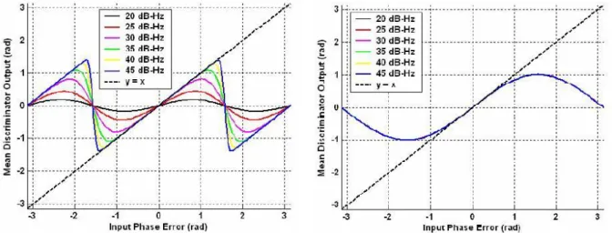
value under which the discriminator does not work in the linear zone, the maximum allowed measurement distortion is reached and thus the discriminator cannot properly measure the phase difference. This value is called the PLL loss of lock threshold since it is considered that under that value the local carrier phase generated by the PLL is no longer accurate enough. A graphical example of the variation of the discriminator linear zone is presented in Figure A-6 [JULIEN, et al. 2005]. This figure shows the slopes of two discriminators, Arctangent and Q, assuming that the discriminator output has been normalized. It can be observed that whereas the arctangent linear zone varies as a function of the pilot channel C/N0, the Q linear
zone remains constant. These curves have been calculated assuming the thermal noise presence only.
Figure A-6: Mean discriminator output (rad) as a function of the input phase error (rad). Left - Arctangent, Right – Q Discriminator. Coherent integration time equal = 4ms. Each of the curves
represents a different value of pilot C/N0 [JULIEN, et al. 2005].
Therefore, from the determination of the linear zone (depends on the accepted degradation of linearity), from the determination of a maximum accepted percentage of phase errors that can
279 fall outside the linear zone and from the knowledge that the phase error variance of the thermal noise depends on the pilot channel C/N0 value, it is possible to calculate the pilot
channel C/N0 value at which the PLL loses its lock.
More specifically, this maximum accepted percentage of phase errors that can fall outside the linear zone has been defined through the phase standard deviation error (σ). Therefore, it has been defined that the PLL loses its lock when 3σ is larger than half the linear zone range [KAPLAN and HEGARTYb, 2006]. In other words, assuming that the tracking error is Gaussian, it is theoretically defined that the PLL conserves its lock for a given C/N0 (PLL
threshold lock) 99% of the time (99% of the time the phase errors fall into the linear zone). Consequently, the pilot channel C/N0 threshold is the pilot channel C/N0 value at which half
the discriminator linear zone is equal to 3σ.
Therefore, the mathematical expression allowing the calculation of the PLL loss of lock threshold when the 4 sources of noise are taken into account is presented below. The mathematical expression is derived from equations (3-5) and (3-6) [KAPLAN and HEGARTYb, 2006]. 2 3 e L (A-26) Where: 2 2 2 Osc Vib th
o σth: Thermal noise standard deviation error
o σVib: Oscillator vibrations standard deviation error
o σOsc: Allan deviation noise standard deviation error θe: Dynamic stress error
Lφ: Two-sided discriminator linear tracking region
From equation (A-26), the PLL loss of lock threshold can be directly calculated.
Table A-1 and Table A-2 [JULIEN, et al. 2005] summarize the threshold values for the different discriminators. These tables are calculated for a TCXO oscillator, for a level of signal dynamics jerk equal to 0 and 1 g/s, and for an effective BL the nearest to 10Hz as
possible. The integration time is 20ms because all the signals have a pilot channel.
Note that the values found in the reference [JULIEN, et al. 2005] are expressed in pilot C/N0
values. Therefore, these values have to be converted to total signal C/N0 values at the receiver
antenna output. The PLL loss of lock threshold expressed in total C/N0 values is given below.
Signal GPS L2C GPS L5 GPS L1C GALILEO E1 OS BL (Hz) Th re sh old (dB -Hz) DOT Product 29 29 27.25 29 7-10 Q 23 23 21.25 23 5-6 Atan 27.5 27.5 25.75 27.5 4-30 Atan2 26 26 24.25 26 2-30
280 Signal GPS L2C GPS L5 GPS L1C GALILEO E1 OS BL (Hz) Th re sh old (dB -Hz) DOT Product 35 35 33.25 35 16-17 Q 29 29 27.25 29 20-30 Atan 27.5 27.5 25.75 27.5 14-30 Atan2 26 26 24.25 26 9-30
Table A-2: PLL tracking loss thresholds with a TCXO oscillator and a jerk = 1 g/s
The first observation to make is that the thresholds values of the Arctangent and Arctangent2 discriminators do not change from Table A-1 and Table A-2. However, this is not entirely true. In fact, each presented threshold is calculated from the BL value inside the specified
range of values which provides the lower PLL loss of lock threshold. Therefore, the BL used
for a determined discriminator is different for each analyzed jerk value. And these BL values
can also be different for each different discriminator. Therefore, in reality, for a given BL, the
PLL loss of lock threshold values of the Arctangent and Arctangent2 discriminators increase when a jerk of 1 g/s is applied.
Another observation is that the product and Arctangent discriminators are only applied over the pilot channel although they could also be used on the data channel. This means that the additional data channel power could also be used to track the signal and thus the threshold should be lower. However, the coherent integration time should be adapted to each GNSS signal since its value should become equal to the signal symbol duration. Therefore, it is not possible to directly add the power of the data channel which has not been used to the pilot channel power in order to calculate the new PLL loss of lock threshold.
The last observation to make is that the thresholds presented in the Table A-2 are calculated assuming that the PLL is always working in the linear region. In fact the bias introduced by the dynamic stress error, expressed in equation (A-25), is only valid when the discriminator is in the linear region. However, there is the possibility that the change in the propagation time between the satellite and the receiver induces a phase change greater than the discriminator linear tracking range during one coherent integration period [JULIEN, et al. 2005]. In other words, the dynamic stress error can provoke by itself a loss of lock. Nevertheless, in this dissertation, it is assumed that the PLL receiver is well dimensioned and that the PLL never loses its lock due to a dynamic stress error bigger than expected. In fact, the assumed value of 1 g/s is very large and hardly a user will receive a signal with a larger jerk; therefore, when the jerk is 1 g/s, the only element which could cause a PLL loss of lock is the thermal noise. Table A-1 and Table A-2 constitute a good reference of PLL tracking threshold values. Nevertheless, these values are calculated from the theoretical noise standard deviation expressions resulting from models where some assumptions were made that are not always fulfilled during the signal tracking process. For example, the BL used in their calculation is
281 A.3.3.4. PLL discriminator selection for the simulations
In this subsection, the PLL discriminator selected to conduct all the simulations of the dissertation is presented. This selection was made from the discriminator performance since one of the objectives of this dissertation is to find the performance bounds of the demodulation of the different GNSS signals. The chosen discriminator is the Q or coherent discriminator and the reasons for its selection are given next.
There are two main reasons which justify the Q discriminator selection. The first reason is that since the majority of the GNSS signals analyzed all along this dissertation have a pilot channel (a dataless channel), it is allowed the utilization of a discriminator which is sensitive to the phase jumps of π introduced by the data because there is no data in the pilot channel. Therefore, since these types of discriminators outperform the discriminators which are insensitive to the phase jumps of π, either the Q or the Arctangent 2 discriminators are chosen. The second reason is that the Q discriminator has a better performance than the Arctangent2 discriminator. This justification is given next.
The main differences between the Costas and Q discriminator with respect to the Arctangent and Arctangent2 discriminators are the following. First, the discriminator normalization factor (KD) of the product and Q discriminators is estimated from the I and Q channels, whereas for
the Arctangent and Arctangent2 discriminators, KD is always 1. Note that this estimation gets
worse with low pilot channel C/N0 levels. Second, whereas the two-sided discriminator linear
region varies as a function of the pilot channel C/N0 for the Arctangent and Arctangent2
discriminators, its value remains constant for the product and Q discriminators.
Therefore, from the previous differences, it is assumed that for low C/N0 levels, the Costas
and Q discriminators have a better performance than the Arctangent and Arctangent2 discriminators. The justification is given next.
For low C/N0 values, the KD estimation of the product and Q discriminators is quite affected
by the thermal noise. Nevertheless, this estimation can be significantly improved when the KD
estimation is made using long periods of time. Obviously, this assumption is only valid when the signal C/N0 does not vary significantly during the KD estimation time. This assumption is
valid for an AWGN channel.
For low C/N0 values, the linear region of the Arctangent and Arctangent2 discriminators is
quite reduced. This region length can be enlarged applying longer coherent integration times. However, the coherent integration time cannot be enlarged indefinitely due to the signal phase variations. In fact, the larger the coherent integration time is, the more the received signal carrier phase can vary between the coherent integration time beginning and the coherent integration time end. Indeed, since the PLL can only provide a linearly varying phase during a coherent integration time period, the integration time size is bounded. And this means that the improvement of the tracking performance of the Arctangent and Arctangent2 discriminators is limited by the coherent integration time.
Therefore, since the tracking performance of the ArcTangent2 discriminator is limited by the coherent integration time, and this time cannot be so easily enlarged as the time used to estimate the KD term, which is the term limiting the tracking performance of the Q
discriminator, the Q discriminator outperforms the ArcTangent2 discriminator from the tracking performance point of view in low C/N0 transmission channels. This statement can be
seen in Table A-1 in spite of the Table A-2 values. Note that the threshold values of Table A-1 and Table A-2 for the different discriminators are calculated for different BL values.
282 Therefore, due to the limited improvement of the tracking performance of the Arctangent and Arctangent2 discriminators for low C/N0 levels and the possibility to use long time periods for
the estimation of the KD normalization factor of the products and Q discriminators, we assume
that the product and Q discriminators have better tracking performance for low C/N0 levels
than the Arctangent and Arctangent2 discriminators. And thus, we choose to implement in the simulations of this dissertation the Q discriminator.
283
Annex B. Figures of merit
In this subsection, three figures of merit are defined. They are the SNR, the Eb/N0 and the
C/N0 and they are used along the entire dissertation. Therefore a good understanding of what
these figures represent, what are their units and what are their inter-relationships is necessary to correctly follow the analyses conducted along the dissertation.
Chapter 10. Rhr(pas effacer)
B.1. Signal-to-noise ratio (SNR)
The signal-to-noise ratio expresses the relationship between the signal power and the noise power [ATIS, 2000]. noise signal P P SNR (B-1)
More specifically, this figure of merit compares the level of a desired signal to the level of background noise. In other words, the SNR represents how much the noise distorts the useful signal. The higher the ratio, the less disturbing the background noise is. The SNR is normally expressed in dB [ATIS, 2000]. noise signal P P dB SNR ( ) 10 log10 (B-2)
Finally, this figure of merit is widely used in the telecommunications field.
B.2. Energy per bit to noise density ratio (E
b/N
0)
The Eb/N0 is an important parameter in digital communication or data transmission. It is a
normalized signal-to-noise ratio (SNR) figure, also known as the “SNR per bit” [ATIS, 2000]. In fact, the relationship between Eb/N0 and SNR is easily calculated. Nevertheless, in order to
establish this relationship, some other figures of merit have to be defined. First, the energy per symbol to noise density ratio (Es/N0) can be approximated as an equivalence to the
signal-to-noise ratio (SNR), where a symbol is the physical representation of a bit or of a group of bits. Indeed, the bits are never directly transmitted through a channel since they belong to the digital domain whereas the channel belongs to the continuous one. Therefore, each bit or group of bits is assigned to a physical waveform in order to adapt the digital signal to its transmission through a channel. This physical waveform is called symbol [PROAKISb, 2001].
The following equation shows the equivalence between the Es/N0 and SNR, an equivalence
which is only true when a matched filter is used to process the received signal [PROAKISc, 2001]. However, the use of the matched filter is the normal strategy followed by any receiver:
SNR P P B N R E N E noise signal s s s 0 0 (B-3) Where:
Rs: Symbol transmission rate B: Channel bandwidth
284 Note that the use of the matched filter sets the channel bandwidth equal to the symbol transmission rate [PROAKISc, 2001]. In fact, the channel bandwidth is the bandwidth of the noise where this noise is the signal noise after the signal processing (filters, etc).
Therefore, since it has been defined that a symbol represents a bit or a group of bits, we can directly relate the Es/N0 with the Eb/N0:
b N E N Eb s 1 0 0 (B-4) Where:
b: Number of bits represented by each symbol
Nevertheless, the bits transmitted through the channel are not the signal information bits. In fact, the information bits are usually encoded by a channel code. The definition of encoding and decoding is given in annex C.3 and C.4. Therefore, Es/N0 is normally related to the
energy per coded bit to noise density ratio (Ec/N0) when a channel code is applied on the
message. Consequently, equation (B-4) may be expressed as: b N E N Ec s 1 0 0 (B-5)
Finally, the Ec/N0 can be related to the Eb/N0 using the code rate, r.
r N E N Eb c 1 0 0 (B-6)
This code rate, r, determines the quantity Y of coded bits needed to represent the quantity X of information bits [PROAKISe, 2001].
Y X
r / (B-7)
To summarize, the final relationship between the SNR and the Eb/N0 is expressed in equation
(B-8) where the Eb/N0 unit is dB [ATIS, 2000]:
b
r dB SNR dB N Eb 10 10 0 log 10 log 10 ) ( ) ( (B-8)Note that, in case that the signal message does not have any channel code, the code rate is equal to 1 and thus the influence of the channel code is cancelled.
This figure of merit is also widely used in the telecommunication field.
B.3. Carrier-to-noise density ratio (C/N
0)
The C/N0 is the ratio between the received carrier power and the receiver noise density [ATIS,
2000]. This figure of merit compares the level of a desired signal to the level of the background noise power density. The advantage of the C/N0 in comparison to the SNR is that
this former figure of merit does not take into account the channel bandwidth (B), and thus it is valid for any signal processing. Note that the signal characteristics and the signal processing inside the receiver determine the channel bandwidth. The relationship between the C/N0 and
285 B SNR N C 0 (B-9)
Therefore, the C/N0 is expressed in dB-Hz [ATIS, 2000]. Moreover, the Eb/N0 and C/N0 can
be related as shown below:
R
b
r dB N E Hz dB N C s b 10 10 10 0 0 log 10 log 10 log 10 ) ( ) ( (B-10)Finally, this figure of merit is widely used in the satellite navigation field.
Chapter 11. hk
287
Annex C. GNSS fundamental processes
In this annex, the definitions of the three main processes conducted by a GNSS receiver are described. These processes are the demodulation of the navigation message, the tracking of the signal and the acquisition of the signal. Additionally, since the demodulation of the navigation message normally implies the decoding of the channel code implemented over the message, the encoding and decoding process of a message are also described.
The descriptions given in this annex are generalized for any type of signal, not only the GNSS signals.
C.1. Signal Demodulation
The demodulation process of a digital communication of a signal consists in estimating the transmitted signal bits values from the antenna output received signal. In other words, the receiver has to decide from the received signal values which is the more probable bit being transmitted [PROAKISc, 2001].
The communication of a digital signal is achieved by transmitting either a waveform or a specific combination of waveforms, where each waveform or specific combination of waveforms represents either a bit or group of bits. This association between bits and waveforms is necessary in order to adapt the digital nature of the bits to the continuous nature of the channel [PROAKISc, 2001].
Therefore, due to the adaptation of the bits to the channel, the receiver must measure the received signal waveforms and/or the received signal waveform amplitudes in order to estimate which waveforms or waveforms amplitudes have been transmitted. And from the estimation of the received signal waveforms and the received signal waveform amplitudes, the transmitted bits can be estimated since the assignation between waveforms and bits at the emission is known [PROAKISc, 2001]. This dissertation calls symbol the set of waveforms and/or the waveform amplitudes assigned to a bit or a group of bits. And the action of assigning a bit or group of bits to a determined signal waveform is called to modulate [PROAKISb, 2001].
Therefore, for an ideal channel, a channel that transmits the signal between the transmitter and the receiver without any kind of distortion or any kind of noise, the estimated symbols at the receiver are identical to the transmitted ones. This means that the transmitted bits are perfectly recovered at reception.
However, in reality, even the simplest channel, the AWGN channel, distorts the received signal after the communication. Therefore, the received signal waveforms and/or the received signal waveform amplitudes no longer correspond to a signal waveform and/or a signal waveform amplitude assigned to a bit or group of bits. Consequently, the receiver has to decide from the received signal waveforms or received signal waveform amplitudes which were the original transmitted symbols. The received signal waveforms or received signal waveform amplitudes are called the channel observations and play an important role into the demodulation of the signal [PROAKISc, 2001].
There are several criterions that can be used to decide which symbol has been transmitted and the most common is the Maximum a Priori (MAP) criterion [PROAKISc, 2001]. This criterion searches the probability of transmitting the symbol si(t), associated to a bit or group
288 of bits, when the signal r(t) has been received. Equation (C-1) represents its mathematical expression:
s (t)r(t)
P i (C-1)
Where:
P(x|y): Probability of x when y occurs
Therefore, the receiver decides that the symbol i has been transmitted if the symbol i has the largest MAP probability among all the possible symbols [PROAKISc, 2001]:
si(t) transmitted P
si(t)r(t)
P
sj(t)r(t)
j0..L1,ji (C-2) Where: L: Number of symbols
However, the probability in (C-1) cannot be directly obtained and thus, this criterion is related to the Maximum Likelihood (ML) criterion by the Bayes theorem [PROAKISc, 2001]. The ML criterion searches the probability of receiving the signal r(t) when the symbol si(t) has
been transmitted. This theorem has an equivalent expression for the probability density function.
r(t)s (t)
f i (C-3)
Where:
f(x): probability density function of x
Therefore, the final MAP expression is [PROAKISc, 2001]: si(t) transmitted
↕
r t s t
P
s t
f
r t s t
Ps t j L j i f ( ) i( ) i( ) ( ) j( ) j( ) 0.. 1, (C-4) In equation (C-4), it can be observed that apart from the observation of the channel, r(t), another factor influences the final symbol decision, the term P(si(t)). This factor is the a priori
information of the signal communication, and altogether with the channel observation, they are the major actors of the symbol estimation process [PROAKISc, 2001].
Finally, one last intuitive concept can be extracted from equations (C-3) and (C-4). These equations show that the detected symbol will be the symbol which is the most similar to the received signal waveforms but weighted by the a priori information.
C.2. Demodulation Performance
The demodulation performance expresses how well a transmitted signal is demodulated: it indicates the quantity of errors made when demodulating the received signal [PROAKISc, 2001]. Obviously, the demodulation performance depends on the transmission channel, the employed demodulation technique, the signal characteristics, etc. All these factors define a scenario with fixed characteristics except for the signal power and the noise power. Therefore, the demodulation performance of a given scenario is given by the quantity of decision errors as a function of the signal power and the noise power [PROAKISc, 2001].
289 The relationship between the signal power and the noise power is provided by the three different figures of merit already defined in 0: the SNR, the Eb/N0 and the C/N0. The Eb/N0 is
the most used figure in the telecommunications field. However, the C/N0 is also used along
this dissertation since it is the reference figure of merit in the satellite navigation field.
The quantity of errors made when demodulating the received signal can be expressed with three different parameters. Each parameter defines the percentage of errors of a different information unit. The parameters are the Bit Error Rate (BER), the Word Error Rate (WER) and the Ephemeris Error Rate (EER).
To sum up, the demodulation performance of the different GNSS signals analyzed in this study is expressed as the BER, the WER and the EER as a function of either the Eb/N0 or the
C/N0.
The BER, the WER and the EER are detailed and their influence is commented below. C.2.1. Bit Error Rate (BER)
The BER is equal to the number of wrong demodulated bits divided by the number of total transmitted bits [ATIS, 2000]. Therefore, the BER expresses the percentage of bits that would be wrong demodulated during the communication of a specific signal through a determined channel. Bits of Number Total Bits Erroneous of Nmmber BER (C-5)
Besides, the BER can be calculated either over the information bits or over the coded bits. The most significant figure of merit is the BER of the information bits since the final user is only concerned by the information, and not on how this information is transmitted [PROAKISe, 2001]. Moreover, the BER of the information bits provides more information than the BER of the coded bits as detailed hereafter.
The BER of the coded bits shows the influence of the transmission channel and the influence of the signal adaptation to the channel (modulation, etc). Moreover, this BER indicates the influence of the energy per bit and, depending on the figure of merit associated to the BER (C/N0 for example), the symbol transmission rate influence. But, in addition to all these
influences, the BER of the information bits also shows the additional protection provided by the channel code implemented over the message.
To sum up, the BER of the information symbols provides the percentage of error on transmitted information bits, which is the only interesting value to the final user, and shows the improvement of the signal demodulation due to the introduction of a channel code. Remember that each GNSS signal has a distinct channel code.
Finally, the BER is a great indicator of the signal design quality in terms of demodulation performance. However, the BER does not specify the level of Eb/N0 or C/N0 necessary to
demodulate a determined information message with a given percentage of success. C.2.2. Word Error Rate (WER)
The information transmitted during a communication is not usually a random stream of bits, but rather a structured unit. In fact, all the bits representing an information field, such as the satellite inclination, are usually transmitted together. And, normally, the information fields are
290 grouped depending on their importance, on their type, etc, forming different units of information. These information units have been called packets or words along this dissertation and a different channel code can be implemented on each different word. Moreover, these words are grouped again forming new structures such as subframes or frames. Then, the process of structuring the information in words or subframes is applied over and over again until a periodic repetition of the structure information is achieved.
Additionally, each word usually carries some information which enables the receiver to detect whether any of the bits forming the word are wrong. Therefore, the receiver is usually able to know if the demodulated word information contains any error. This means that it is possible to measure the percentage of times that a word is correctly demodulated. And, even if a word did not carry any information allowing the verification of its integrity, it is always interesting to know the percentage of times that a word can be demodulated without error.
Therefore, the WER is a very interesting figure of merit in terms of percentage of times that an information field can be demodulated without errors. Moreover, the WER shows the influence of the word size because when a word is larger, a better channel code can be implemented. This statement was demonstrated by Shannon [PROAKISd, 2001].
More specifically, the WER is equal to the number of wrong demodulated words divided by the number of total transmitted words [ATIS, 2000].
Words of Number Total Words Erroneous of Nmmber WER (C-6)
Therefore, the WER expresses the percentage of words that would be wrong demodulated during the communication of a specific signal though a determined channel.
Note that the WER can be calculated for each different word transmitted by the signal. However, if the only difference among words is their position inside the signal structure, their WER is the same.
C.2.3. Ephemeris Error Rate (EER)
During the description of the WER, it was said that the information fields are usually grouped into words. Moreover, it was commented that this regrouping is done among information fields providing the same type of information. This is the case of the different GNSS signals, where the information fields containing the satellite broadcasting ephemeris set or clock error corrections are transmitted into the same words. The entire ephemeris data set can be divided into several words as it is done for GPS L1 C/A, GPS L2C [ARINC, 2004], GPS L5 [ARINC, 2005] and GALILEO E1 [ESA, 2008] signals, or all the information can be grouped into only one word as it is done for GPS L1C [ARINC, 2006].
In any case, since the ephemeris and clock data are the only information necessary to obtain the satellite position and thus the final user position, the only important figure of merit from the point of view of the final user is the EER.
Consequently, in this dissertation, the EER is defined as the percentage of times that a receiver can correctly demodulate the signal ephemeris data set. And the EER is calculated by dividing the number of wrong demodulated ephemeris data sets by the number of total transmitted ephemeris data sets.
291 Sets Data Ephemeris of Number Total Sets Data Ephemeris Erroneous of Number WER (C-7)
Note that the Ephemeris Error Rate and the Word Error Rate are equal for the GNSS signals transmitting the ephemeris set and clock data into only one word. Therefore, for the signals transmitting the satellite ephemeris data set into more than one word the only interest of the WER is the following: to compare the value of either Eb/N0 or C/N0 necessary to obtain a
given WER value with the value of either Eb/N0 or C/N0 necessary to obtain a EER value
equal to the WER value. From this comparison, it can be concluded whether the ephemeris data set division into several words has improved the signal demodulation performance.
C.3. Signal Encoding
The encoding of the signal message is the application of a channel code over the signal message. This process consists in introducing, in a controlled manner, some redundancy in the binary information sequence of the signal. This redundancy can be used at the receiver level to overcome the effects of noise and interference encountered in the transmission of the signal through the channel [PROAKISd, 2001]. In other words, from the information bits point of view, the encoding process generates some new bits which represent the same content as the information bits. Therefore, these new bits are redundant since the original information content is already transmitted by the information bits. And the inclusion of these new binary bits into the transmitted word means that if some of the original information bits are corrupted or lost at the reception, the receiver will still have the possibility to recover the message since the lost information could be reconstructed from these new generated bits.
Moreover, in addition to generating the new bits and introducing them to the transmitted word, the information bits can be modified during the encoding process. Therefore, the encoding process can be seen as a generation of a new binary word from the original binary information word, where the original word can be preserved or not. These bits of the new binary word are called coded bits and the new binary word is called coded word [PROAKISd, 2001]. Besides, note that the coded binary word is the binary word used to modulate the signal. Therefore, when a channel code is applied, equation (B-5) is used instead of equation (B-4).
Additionally, the ratio between the size of the original information word and the size of the coded word is called code rate (r). Its expression has already been given in equation (B-6).
C.4. Signal Decoding
The decoding of the received signal message is the action of exploiting the available redundancy contained into the received message in order to correct the perturbations introduced by the channel [PROAKISd, 2001]. Therefore, due to this correction, the receiver can try to recover the original binary information word.
Nevertheless, there are two types of decoding process depending on the decoder block input. In fact, the received signal passes through a demodulator and a detector before entering the decoder [PROAKISd, 2001], as depicted below.
292
Figure C-1: Digital Communication block scheme
The demodulator block processes the received channel-corrupted waveform and reduces each waveform to a scalar or to a vector that represents an estimate of the transmitted data symbol. The detector block quantizes the output of the demodulator block and from this quantization the two possible decoding types are defined [PROAKISd, 2001].
If the number of quantization steps is equal to the number of possible symbols, the detection process has already chosen the symbol and thus has set the binary value of the coded bits. Therefore, since these coded bits are directly fed to the decoder block, this type of decoding is called hard decision. If the level of quantization is infinite, or much larger than the number of symbols, the value of the decoded bits is not binary but real. Therefore, this type of decoding is called soft decision [PROAKISd, 2001].
C.4.1. Strategies of channel codes use
There are two different strategies of channel code use. The first one is called Forward Error Correction (FEC) and consists in using the redundancy transmitted into the signal message in order to correct any possible errors introduced by the channel [PROAKISe, 2001].
The other use is called Automatic Repeat-Request (ARQ). It consists in detecting if any error has been introduced by the transmission channel into the received signal and in asking the transmitter to resend the information if some error was detected [PETERSON and DAVIE, 2003]. Along this Ph.D. manuscript, the action of using the word channel code to detect if the word contains any erroneous bit has been called verification, and the verification process is called verify the channel code. Therefore, if a word fails the channel code verification, it means that the word contain erroneous bits. And, if a word passes the channel code verification, it means that the word is error free.
In satellite navigation systems, the ARQ is not possible since the transmitters are only a few satellites whereas the number of receivers is much bigger. Therefore, a single receiver cannot request the retransmission of the navigation message. Nevertheless, the ephemeris data set is continuously repeated during a period of time, and when another set replaces the previous one, the user no longer needs the first ephemeris data set. Therefore, even if the user does not correctly decode an ephemeris data set, a retransmission request is unnecessary since the needed information is continuously broadcasted by the satellite [SPILKER and ASHBYb, 1996]. However, even if the ARQ strategy is not implemented, each GNSS signal has a channel code allowing the verification of the received words as seen in 0. And normally, if the word verification fails, the word is discarded.
Finally, in addition to the channel code used to detect whether the word is error free or not, the majority of GNSS signals have another channel code used to implement the FEC as it has also been seen in 0.
![Figure D-2: Desinterleaver GPS L1C navigation message [ARINC, 2006]](https://thumb-eu.123doks.com/thumbv2/123doknet/3710663.110474/45.892.181.700.688.1033/figure-d-desinterleaver-gps-l-navigation-message-arinc.webp)
![Figure D-5: Even or Odd Part of a Page Structure Galileo E1 OS [ESA, 2008]](https://thumb-eu.123doks.com/thumbv2/123doknet/3710663.110474/48.892.173.738.739.906/figure-even-odd-part-page-structure-galileo-esa.webp)
![Figure D-7: Subframe Structure Galileo E1 OS [ESA, 2008]](https://thumb-eu.123doks.com/thumbv2/123doknet/3710663.110474/50.892.109.783.589.852/figure-subframe-structure-galileo-e-os-esa.webp)