Combined Estimation of Material Law and Unloaded Configuration (Application to Pulmonary Poro-Mechanics)

(1)

HAL Id: hal-03043448

https://hal.inria.fr/hal-03043448

Submitted on 14 Jan 2021

HAL is a multi-disciplinary open access archive for the deposit and dissemination of sci-entific research documents, whether they are pub-lished or not. The documents may come from teaching and research institutions in France or abroad, or from public or private research centers.

L’archive ouverte pluridisciplinaire HAL, est destinée au dépôt et à la diffusion de documents scientifiques de niveau recherche, publiés ou non, émanant des établissements d’enseignement et de recherche français ou étrangers, des laboratoires publics ou privés.

Combined Estimation of Material Law and Unloaded

Configuration (Application to Pulmonary

Poro-Mechanics)

Mahdi Manoochehrtayebi

To cite this version:

Mahdi Manoochehrtayebi. Combined Estimation of Material Law and Unloaded Configuration (Ap-plication to Pulmonary Poro-Mechanics). Mechanical engineering [physics.class-ph]. 2020. �hal-03043448�

(2)

M

ASTER

T

HESIS

Combined Estimation of Material Law

and Unloaded Configuration

Application to Pulmonary Poro-Mechanics

Author:

Mahdi MANOOCHEHRTAYEBI

Supervisor: Martin GENET

Solid Mechanics Laboratory ÉCOLE POLYTECHNIQUE(IP PARIS)

(3)

(4)

A

BSTRACT

T

he human body acts as a complicated mechanical system. One of the subsystems in the human body is the respiratory system, which contains the lung and the thorax. Simulating this system as a mechanical system, mechanical properties, like stiffness for the lung, can be considered. Our lungs are under mechanical load by air. In the inhalation and exhalation process, the lung geometry passes through different configurations, but never the unloaded configuration. Fining this unloaded configuration is an interesting problem in biomechanics. In this paper, different mechanical systems have been studied, and methods for finding the unloaded configuration have been suggested, which are applied for solving such a problem for the lung. In this paper, it has been shown that estimating the unloaded configuration, one data point, which contains a loaded configuration and the corresponding applied force, is needed. and for material parameter estimation, if the dimension of the problem is more than the quantity of the material parameters, one data point is enough for material parameters estimation, too.

In this article, the inverse problem for the linear and nonlinear spring, Rivlin cube, tube, and at the end, the lung mechanical modeling has been discussed. The inverse problem is divided into the unloaded configuration and material parameter estimation. Methods used for solving the nonlinear equations are the gradient-free method, Newton nonlinear solver, and the gradient descent method. Moreover, the priority of the Newton solver has been shown.

The novelty studied in this project combines two classic problems in mechanics, and here the combined estimation of the material parameters and unloaded configuration has been discussed. In the end, the application of this estimation in lung pro mechanic has been studied. For modeling the lung mechanics, CT1(x-ray based) images during the inhalation and exhalation process for the hospital patients have been used.

(5)

(6)

A

CKNOWLEDGMENTS

Acknowledgments

R

eaching to this peak of science, I was the smallest part of this power system, which pushed me here. First and foremost, all the honors and appreciations belong to my family, who tried more than me to reach up to here. I’m fortunate to have such a family and passed through a way in which I have become familiar with great people; each of them has played a role in my success.

In my master’s internship period, it was time to start dealing with science, which is a very different way compared with what I was studying before. I am so grateful that I entered the science world under the supervision of Prof. Martin Genet, who made my mindset in the way of research, especially during this epidemic period in which I had to do almost all of my internship period at home; he was always accessible and in touch with me.

Besides Prof. Martin Genet, Cecile Patte has a significant portion of this project who shared her three-year Ph. D. research results and had much time training me. Many thanks to Dr. Taghvaeipour, Dr. Kamali, Prof. Michael Jabbour, Prof. Domonique Chapelle, École Polytechnique solid mechanics laboratory, Active M3DISIM team, and INRIA.

(7)

(8)

A

UTHOR

’

S DECLARATION

I

, Mahdi MANOOCHEHRTAYEBI, declare that this thesis titled, ’Combined Estimation of Material Law and Unloaded Configuration’ and the work presented in it is my own. I confirm that this work submitted for assessment is my own and is expressed in my own words. Any uses made within it of other authors’ works in any form (e.g., ideas, equations, figures, text, tables, programs) are appropriately acknowledged at any point of their use. A list of the references employed is included.

(9)

(10)

T

ABLE OF

C

ONTENTS

Page

List of Figures ix

1 Introduction 1

2 Combined Estimation of Material Parameters and Unloaded Configurations 7

2.1 Models . . . 7 2.1.1 Linear Spring . . . 7 2.1.2 Nonlinear Spring . . . 8 2.1.3 Rivlin Cube . . . 8 2.1.4 Tube . . . 10 2.2 Forward Problem . . . 11

2.2.1 A Method for Solving Nonlinear Problems. . . 11

2.2.2 Linear Spring . . . 12

2.2.3 Rivlin Cube . . . 12

2.3 Inverse Problem . . . 22

2.3.1 Methods for Minimizing a Cost Function. . . 23

2.3.2 Methods for Computing Gradients and Hessians . . . 24

2.3.3 Unloaded Configuration Estimation . . . 29

2.3.4 Material Parameter Estimation . . . 30

2.3.5 Combined Estimation of the Unloaded Configuration and Material Para-meters . . . 34

2.4 Finite Differences Approximation of the Derivative and Hessian Matrix . . . 40

2.4.1 Computing the Gradient of Some Functions. . . 40

3 Lung Mechanical Modeling 45 3.1 Introduction . . . 45

3.1.1 Lung Mesh. . . 45

3.1.2 Thorax Mesh . . . 45

3.1.3 Lung Porosity . . . 46

(11)

TABLE OF CONTENTS

4 Discussion and Ongoing Research 51

Bibliography 53

(12)

L

IST OF

F

IGURES

FIGURE Page

1.1 Sketch of the general forward mechanical problem [12]. . . 2 1.2 Illustration of Sellier’s iterative method for identifying a stress-free reference

configu-ration in biomechanical boundary value problems [11]. . . 2 1.3 Schematic of the reference configuration and the deformed configuration with the

associated local quantities, volumes and porosity [9]. . . 3 1.4 Kinematics of pre-strained biological systems. Pre-strain maps the stress-free

refer-ence configuration onto the residually stressed but mechanically unloaded configura-tion [3]. . . 4

2.1 Minimization of the cost function of the nonlinear spring with respect to the material parameters . . . 9 2.2 Tube geometry by Martin Genet in two different time steps under different loading

pressures . . . 10 2.3 The variation of Rivlin cube configuration and stress for the Saint Venant-Kirchhoff

model under the applied axial compression in the x- direction. . . 14 2.4 The variation of the Rivlin configuration and stress with respect to the equitriaxial

pressure applied on the compressible Saint Venant-Kirchhoff model. . . 14 2.5 The variation of Rivlin cube configuration and stress with respect to applied axial

pressure for the compressible Mooney-Rivlin model . . . 18 2.6 The variation of Rivlin cube configuration and stress with respect to applied

equireiax-ial pressure for the compressible Mooney-Rivlin model . . . 18 2.7 The variation of Rivlin cube configuration and stress with respect to applied axial

pressure for the incompressible Mooney-Rivlin model . . . 19 2.8 The variation of Rivlin cube configuration and stress with respect to applied

equireiax-ial pressure for the incompressible Mooney-Rivlin model. . . 19 2.9 Three different bulk energy models variation with respect to the compression index . 20 2.10 First derivative of three different bulk energy models variation with respect to the

(13)

LIST OF FIGURES

2.11 Second derivative of three different bulk energy models variation with respect to the

compression index . . . 22

2.12 The variation of the pressure and displacement with respect to the lambda for the compressible Saint Venant-Kirchhoff model . . . 30

2.13 Minimizing the cost function (J(E)) by CMA code for the linear spring. . . 31

2.14 The variation ofλin Saint-Venant Kirchhoff model with respect to the applied equitri-axial pressure applied on Rivlin Cube . . . 32

2.15 The variation of Rivlin cube configuration and stress with respect to applied axial pressure for the incompressible Saint-Venant Kirchhoff model . . . 32

2.16 The variation of Rivlin cube configuration and stress with respect to applied equitriax-ial pressure for the incompressible Saint-Venant Kirchhoff model . . . 33

2.17 Minimization of Mooney-Rivlin cube cost function with respect to re-scaled material parametersλandµ. . . 34

2.18 Minimization of Mooney-Rivlin cube cost function with respect to re-scaled material parametersλandµ. . . 35

2.19 Linear spring cost function minimization with respect to the re-scaled parameters of the unloaded configuration and Young modulus . . . 37

2.20 Minimization of the cost of the linear spring with respect to two parameters of the unloaded configuration and stiffness coefficient . . . 38

2.21 Minimization of Mooney-Rivlin cube cost function with respect to re-scaled material parametersλandµand unloaded configuration parameters. . . 38

2.22 Tube cost function minimization for the unloaded configuration and material parame-ter estimation via CMA code. . . 39

2.23 Tube cost function minimization for the unloaded configuration and material parame-ter estimation via Newton method. . . 39

2.24 Tube cost function minimization for the unloaded configuration and material parame-ter estimation via gradient descent method. . . 40

3.1 Lung surface mesh obtained in MeVisLab. . . 46

3.2 Lung 3D mesh obtained in GMSH from the surface mesh . . . 47

3.3 Lung CT images in three different angles . . . 47

3.4 Thorax surface mesh obtained in MeVisLab . . . 48

3.5 Thorax 3D mesh obtained in GMSH . . . 48

3.6 CT image before and after porosity consideration . . . 49

3.7 The right lung with different values of porosity. Blue color shows zero porosity and red color show parts with porosity equal to one. . . 49

3.8 Thorax mask images in three different angles . . . 50

3.9 Thorax displacement field from end of the exhalation process and end of the inhalation process. . . 50

(14)

C

H A P T E R

1

I

NTRODUCTION

O

ne classic problem in biomechanics is solving the inverse problem for a biomechanical system when the unloaded configuration or the material parameters are unknown. The new problem discussed here is the combined estimation of the unloaded configuration and material parameters. One of the exciting problems discussed in this paper will be developed later is to solve such a lung problem. This problem can be simulated to a mechanical system by finite element methods and considering a stiffness for it as a mechanical property where the controlling force is the air pressure.

In this chapter, some simple 1D to 3D problems have been discussed. In the end, the methods have been generalized for a more complicated problem like the tube, which has an n-dimensional configuration, making it more complicated to find a solution for the unloaded configuration.

The last model that has been discussed in this project is the lung poromechanic. The purpose of what has been discussed before is to model and find a lung poromechanics solution as the lung contains blood and air as the liquid in it. Besides the lung, the thorax plays an essential role in respiration, which is always in contact with the lung. So, thorax displacement can affect the inhalation and exhalation process.

Literature Review

For solving the inverse problem in hyperelasticity, different methods have been proposed. First of all, it is necessary to consider a re-parameterization of the weak form of the forward problem of finite elasticity as a solution method for the inverse incompressible problem. Many numerical approaches have been proposed for solving forward problems in incompressible finite elasticity. Most commonly, a mixed formulation is assumed with independent fields for displacements,

(15)

CHAPTER 1. INTRODUCTION

pressure, and sometimes the volumetric deformation[7].

The material used in this paper and cites govindjeecom putational1998istheN eo−HookeanmaterialwiththecompressibleCiarletGe ymonatconstitutiverelationshi p [6].F orsolvingsuchproblemsnumericall y, itisneededtominimizeacost f unction [1].So, therewouldsuggestaniterativemethod f orminimizingsuchacost f unction f oraprobleminwhich f orcesareappliedintheboundar y [12]asshowninF i gure1.1.

Figure 1.1: Sketch of the general forward mechanical problem [12].

The methods used in [12] has been implemented for a problem which contains fluid like what is discussed in the next chapter [11] as in Figure1.2. The concept of the inverse problem in hyperelasticity is what is proposed in [2].

Figure 1.2: Illustration of Sellier’s iterative method for identifying a stress-free reference configu-ration in biomechanical boundary value problems [11].

.

The concept of the inverse problem in hyperelasticity is what is proposed in [2].

As discussed in the last chapter, the inverse problem can be solved for the multi-dimensional problems if there are as many data points as needed. The same problem can be solved for the lung, but there are other aspects of this problem: the existence of the thorax and the porosity in the lung.

In [9], the lung’s inverse problem by considering the porosity and poromechanics theory for large

(16)

deformations has been discussed hyperelastic potential reproducing the volumetric response of the pulmonary mixture to a change of pressure has been studied.

Figure 1.3: Schematic of the reference configuration and the deformed configuration with the associated local quantities, volumes and porosity [9].

A similar method has been discussed for the heart. The proposed method is embedded within the continuum theory of fictitious configurations and uses a fixed-point iteration on the geometry itself [3].

The motivation to work on the lung is its importance on human health as there are many pulmonary diseases. For example, a chronic disease in which collagen fibers accumulate into interstitial tissue leads to thickening, stiffening, and damage of alveolar walls. This disease remains poorly understood, poorly diagnosed, and poorly treated and represents a real clinical challenge. In interaction with data such as medical imaging, mechanical modeling-based tools could help clinicians in classifying patients and thus deciding on the treatment options [8]. For modeling the lung from the CT images, images registration tools have been implemented [4]. In the lung problem, the lung is in contact with the thorax, so the boundary problem by consid-ering the contact between the lung and thorax should be considered in the boundary condition problem [10]. In [5], image processing has been implemented for the heart problem for extracting ventricular strain data from MR images.

(17)

CHAPTER 1. INTRODUCTION

Figure 1.4: Kinematics of pre-strained biological systems. Pre-strain maps the stress-free refer-ence configuration onto the residually stressed but mechanically unloaded configuration [3].

Types of the Problems Discussed

This chapter will start with the most simple problem, which is the linear spring. This problem has a one-dimensional configuration, which is the length of the spring. And also, there is stiffness for this spring as its material parameter.

Assumptions for obtaining the unknown material parameter and unloaded configuration is that the spring’s length under an applied force has been measured. So, two applied forces with the corresponding deformed length are needed two obtain these two unknowns.

Different methods for solving this problem are implemented and generalized for a nonlinear spring and a three-dimensional problem, which is the Rivlin cube. For Rivlin cube, different material laws have been studied, and the more practical one is introduced. All the different methods have been implemented in the tube problem with the n-dimension configuration, and the more efficient one is introduced.

Materials and Methods

In mechanical systems, we may face problems in which the initial (unloaded) state is known, plus the material parameters. In this situation, the configuration under a specific load can be determined.

There are some unknown parameters, while these parameters like deformed configuration in these kinds of problems are known. Moreover, this deformed configuration is typically measured from the imaging data. So, there would be a cost function like Equation (1.1), which shows that

(18)

the parameter_θis the actual value when making the cost function minimum, which is equal to zero. (1.1) θ= argmin ½ J(θ) =1 2 Z

Ωmes(U(θ) −U

mes₎2¾

So, the goal is to minimize the cost function, which varies from problem to problem. Never-theless, the critical point is that the suggested cost function needs at least as many terms as the unknown parameters. There are different ways to minimize such a cost function, containing unknown parameters such as the material parameters or the unknown configurations. The unknown configuration depends on the problem dimension; for instance, it is one for a linear spring and three for a cube with three different dimensions.

(19)

(20)

C

H A P T E R

2

C

OMBINED

E

STIMATION OF

M

ATERIAL

P

ARAMETERS AND

U

NLOADED

C

ONFIGURATIONS

Introduction

In this chapter, the inverse problem has been discussed for different models, and different methods have been implemented for solving the nonlinear equations. The inverse problem contains two aspects of the unloaded configuration and material parameter estimation, estimated together. Before going to the inverse problem concept, the forward problem has been explained. In the end, the minimization of the cost function has been discussed and methods of doing it.

2.1 Models

Materials discussed in this paper are linear and nonlinear spring, Rivlin cube, and a tube. Each of them has its material parameters and coordinates, which are discussed in the following.

2.1.1 Linear Spring

A linear spring is the most straightforward problem which can be discussed here. The linear spring has only a stiffness coefficient and a length, which changes by applying a force. In general, the linear spring law can be written as below:

(2.1) E¡ud e f− uund e f¢ = F

E is the stiffness coefficient, F the applied force, and u_{und e f} and u_{d e f} are the undeformed and deformed length, respectively.

(21)

CHAPTER 2. COMBINED ESTIMATION OF MATERIAL PARAMETERS AND UNLOADED CONFIGURATIONS

2.1.2 Nonlinear Spring

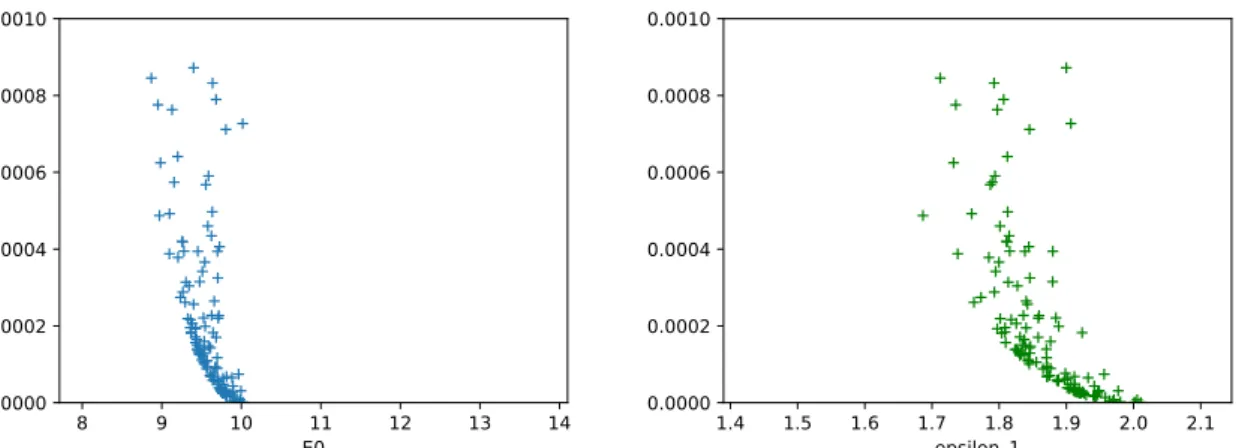
For the linear spring, there was only one material parameter, which was the young modulus. For the nonlinear spring, there are two parameters for the nonlinear spring, which law is as mentioned below: (2.2) _σ_{= E(²) ·}_² (2.3) E(_{²) = E}₀e²1² (2.4) _σ_{= E}0e ² ²1 _{· (²}₋_²₀)

Three data points are needed for solving the inverse problem and material parameters for this geometry as there are two parameters as material parameters. The solving method is a bit different here, though the CMA1 algorithm has been used again. For solving this problem with three data points and three unknown parameters, the solving process can be started from a known configuration with the applied force, different values for E0 and²1 can be guessed, which

are the material parameters.

There are three deformed configurations with measured forces. So, the solving process can be started with one of the known configurations and with the guessed material parameters, and the unloaded configuration can be computed by it. There are an unloaded configuration and two measured forces with which two corresponding loaded configuration can be computed. Here, the cost function is defined as calculating the difference between the measured deformed configuration and the calculated ones. The minimization of the cost function concerning the material parameters are shown in the Figure2.1

2.1.3 Rivlin Cube

What is mentioned simply for spring can be generalized for a 3D cube, which has three different dimensions, and any vector force can be applied on each aspect with different values that can deform the shape of the cube. If we applied force on a different aspect of such a cube, there would be deformation on each side. For example, if we apply forces on a cube with dimensions of:

(2.5) _{X 0 =}     x y z    

1_{Covariance Matrix Adaptation}

(22)

2.1. MODELS 8 9 10 11 12 13 14 E0 0.0000 0.0002 0.0004 0.0006 0.0008 0.0010 J

(a) Minimization if the cost function with respect to the material parameter E0

1.4 1.5 1.6 1.7 1.8 1.9 2.0 2.1 epsilon_1 0.0000 0.0002 0.0004 0.0006 0.0008 0.0010 J

(b) Minimization if the cost function with respect to the material parameter²1

Figure 2.1: Minimization of the cost function of the nonlinear spring with respect to the material parameters

After deforming such a cube under the force applied, the dimensions of the cube would be deformed as below: (2.6) _{X 1 =}     λ1x λ2y λ3z    

Here we define matrix F which is the deformation gradient.

(2.7) _{F =}     λ1 0 0 0 λ2 0 0 0 λ3    

The right Green-Cauchy tensor C and the left Green-Cauchy tensor b are as below:

(2.8) _{C = F}T_{· F =}     λ2 1 0 0 0 λ2₂ 0 0 0 λ2₃     (2.9) _{b = F · F}T=     λ2 1 0 0 0 _λ2₂ 0 0 0 λ2₃     And E is the Green-Lagrange strain tensor.

(2.10) _{E =}C − I 2 =      λ2 1−1 2 0 0 λ2 2−1 2 0 S ym λ 2 3−1 2     

(23)

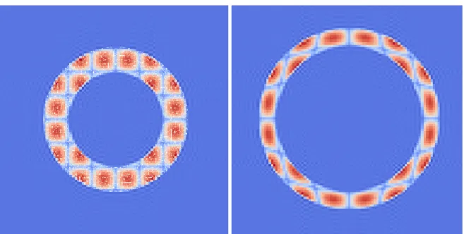
(a) Unloaded configuration of the tube (b) Loaded configuration of the tube

Figure 2.2: Tube geometry by Martin Genet in two different time steps under different loading pressures

In which "I" is the identity tensor:

(2.11) _{I =}     1 0 0 0 1 0 0 0 1    

It is evident that the stress tensor is obtained from the derivative of the energy form. So, what we choose as our energy model can change the stress tensor.

2.1.4 Tube

Here a 2D tube has been discussed, which has an inner radius and an outer radius. This problem is symmetric and has a constant young modulus. The input of the problem is the tube inner pressure, which makes inflation of the tube.

This 2D problem is multi-dimensional in that it would be parameterized by the finite element method, and the node displacements would be the configuration of the problem. There is the young modulus as the material parameter for the tube problem and the unloaded configuration. There are some time steps, which are the configurations of the tube for different values of the inner pressure. In Figure2.2, the first and last loaded configuration has been shown.

(24)

2.2. FORWARD PROBLEM

2.2 Forward Problem

This kind of problem is not very common to solve. The meaning of the forward problem is that we change the model configuration and see what forces correspond to the new configuration. In the real problem, this is rarely happening, or it may only be calculated to see the force needed to obtain the ideal configuration. In the following, the forward problem is demonstrated for the models discussed in this paper.

2.2.1 A Method for Solving Nonlinear Problems

For the hyperelastic model the stress tensorσ(λ) should be equal to the applied pressure P, but as an initial guess like_λ₀ we have a residual which is the difference between the stress tensor and the applied pressure vector:

(2.12) R₀₌_σ(_λ₀_{) − P} In the above equation,σand P are defined as below:

(2.13) σ=     σ11 σ22 σ33     (2.14) _{P =}     P1 P2 P3     And: (2.15) R₀₌     σ11− P1 σ22− P2 σ33− P3    

Using Taylor expansion aroundλ0, we can obtain the update law.

(2.16) σ(λ0+∆λ) ≈σ(λ0) +

∂σ

∂λ(λ0) ·∆λ As there is:

(2.17) σ(λ0+∆λ) = P

So, the update law would be like Equation (2.90)

(2.18) ∆λ0=

P −σ(λ0)

∂σ

∂λ(λ0)

(25)

In which Jac is Jacobian matrix of_σ:

(2.19) _{Jac =}∂σ

∂λ

What has been done here is that the cost function should be minimized, which means that its gradient should become zero. So, the newton method has been done on the derivative of the cost function.

2.2.2 Linear Spring

For a linear spring, The forward problem is such that the stiffness coefficient, applied force, and the undeformed length is known, and the only unknown is the deformed length, which can be obtained by the following relation:

(2.20) ud e f_{= u}undef₊F E

2.2.3 Rivlin Cube

What is mentioned simply for spring can be generalized for a 3D cube, which has three different dimensions, and any force vector can be applied on each face with different values that can deform the shape of the cube. If a force is applied to different aspects of such a cube, there would be deformation on each side. For example, the mentioned force can be applied on a cube by following dimensions: (2.21) _{X 0 =}     x y z    

After deformation of such a cube under the force applied, the dimensions of the cube would be deformed as below: (2.22) X 1 =     λ1x λ2y λ3z    

Here matrix F which is the deformation gradient can be defined as below:

(2.23) _{F =}     λ1 0 0 0 λ2 0 0 0 λ3    

2.2.3.1 Saint Venant-Kirchhoff Model

Saint Venant-Kirchhoff energy model is like the (Equation (2.24))

(2.24) Ψ =λ

2(tr E)

2_+µ_{(tr E}2₎

(26)

Stress tensor for compressible material can be obtain by derivative of the energy function.

(2.25) Σ =∂Ψ ∂E =λ(tr E)I + 2µE (2.26) σ= 1 JF Σ F T =     σxx 0 0 σy y 0 S ym σzz    

The stress components are:

(2.27) σxx= λ1[(λ+ 2µ)λ2₁+λ(λ2₂+λ2₃) − 3 − 2µ 2λ2λ3 (2.28) σy y= λ2[(λ+ 2µ)λ2₂+λ(λ2₁+λ2₃) − 3 − 2µ 2λ1λ3 (2.29) σzz= λ3[(λ+ 2µ)λ2₃+λ(λ2₁+λ2₂) − 3 − 2µ 2λ1λ2

And also the compressibility index:

(2.30) _{J =}_λ₁_λ₂_λ₃

For such a model we do a test by pulling it in the x - direction. So, the boundary conditions can be defined as below:

(2.31) _σ_{· (±e}_x_{) = F e}_x

(2.32) σ_{· (±e}y) = 0

(2.33) σ_{· (±e}z) = 0

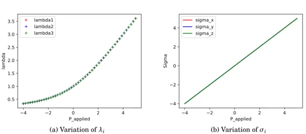
The test done on this model is pulling the cube in the x-direction. This test has been done by applying tension from -0.2 MPa to 0.4 MPa. The results are shown in the Figure2.3.

To solve the inverse problem for different applied force values, a numerical solver is needed to solve the equation and numerically obtain the inverse values. So, we implemented a Newton solver, and in the end, we compared it with the Newton solver of the Python library.

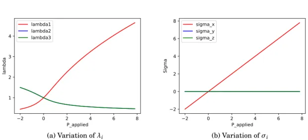
In Figure2.4Saint Venant-Kirchhoff model shows logical responses for equitriaxial loading, which means that the more compression, the stiffer the material.

(27)

CHAPTER 2. COMBINED ESTIMATION OF MATERIAL PARAMETERS AND UNLOADED CONFIGURATIONS 0.2 0.1 0.0 0.1 0.2 0.3 0.4 P_applied 0.80 0.85 0.90 0.95 1.00 1.05 1.10 1.15 1.20 lambda lambda1 lambda2 lambda3 (a) Variation ofλi 0.2 0.1 0.0 0.1 0.2 0.3 0.4 P_applied 0.2 0.1 0.0 0.1 0.2 0.3 0.4 Sigma sigma_x sigma_y sigma_z (b) Variation ofσi

Figure 2.3: The variation of Rivlin cube configuration and stress for the Saint Venant-Kirchhoff model under the applied axial compression in the x- direction

4 2 0 2 4 P_applied 0.5 1.0 1.5 2.0 2.5 3.0 3.5 lambda lambda1 lambda2 lambda3 (a) Variation ofλi 4 2 0 2 4 P_applied 4 2 0 2 4 Sigma sigma_x sigma_y sigma_z (b) Variation ofσi

Figure 2.4: The variation of the Rivlin configuration and stress with respect to the equitriaxial pressure applied on the compressible Saint Venant-Kirchhoff model

(28)

2.2.3.2 Mooney-Rivlin Model

Mooney-Rivlin energy model is proposed as Equation (2.34)

(2.34) Ψ = c1(IC− 3) + c2(I IC− 3) +κ(J2− 1 − 2 ln J)

Which quantities are defined as below:

(2.35) IC= J− 2 3_I_C (2.36) I IC= J− 4 3_{I I}_C (2.37) _{C = J}−23_C (2.38) _{F = J}13_F

For obtainingΣ the following equation can be used:

(2.39) Σ =∂Ψ ∂E = 2 ∂ψ ∂C = 2 ∂Ψ ∂I_C ∂I_C ∂C + 2 ∂Ψ ∂I I_C ∂I I_C ∂C + 2 ∂Ψ ∂J ∂J ∂C

By the chain rule:

(2.40) ∂IC ∂C = ∂I_C ∂J ∂J ∂C (2.41) ∂J ∂C= J 2C −1 As a result: (2.42) ∂IC ∂C = J −23 µ I −IC 3 C −1 ¶ (2.43) ∂I IC ∂C = J −43 µ ICI − C − 2 3I ICC −1¶

For compressible material:

(2.44) Σ = 2C1J− 2 3 µ I −IC 3 C −1¶_{+ 2C} 2J− 4 3 µ ICI − C − 2 3I ICC −1¶_{+ 2κ}_(J2 − 1)C−1 (2.45) σ₌ 1 JF S F T

(29)

CHAPTER 2. COMBINED ESTIMATION OF MATERIAL PARAMETERS AND UNLOADED CONFIGURATIONS So: (2.46) σ_{= 2C}1J− 5 3 µ b −IC 3 I ¶ + 2C2J− 7 3 µ ICb − b2− 2 3I ICI ¶ + 2κ(J −1 J)C −1

It can be supposed c1= c2= cK. So,σwill be:

(2.47) _σ_{= 2c}_K · J−53 µ b −IC 3 I ¶ + J−73 µ I_C_{b − b}2₋2 3I ICI ¶¸ + 2κ(J −1 J)C −1

For the incompressible model (J = 1) and the following relations are true:

(2.48) σxx= 2cK " λ2 1− λ2 1+λ22+λ23 3 + ¡ λ2 1+λ22+λ23 ¢ λ2 1−λ41− 2 3 ¡ λ4 1+λ42+λ43 ¢ # −γ (2.49) σy y= 2cK " λ2 2− λ2 1+λ22+λ23 3 + ¡ λ2 1+λ22+λ23 ¢ λ2 2−λ42− 2 3 ¡ λ4 1+λ42+λ43 ¢ # −γ (2.50) σzz= 2cK " λ2 3− λ2 1+λ22+λ23 3 + ¡ λ2 1+λ 2 2+λ 2 3 ¢ λ2 3−λ 4 3− 2 3 ¡ λ4 1+λ 4 2+λ 4 3 ¢ # −γ

In which_γis the hydro-static pressure. For the incompressible model another relation exists:

(2.51) _{J =}λ1λ2λ3= 1

By applying the boundary conditions as below:

(2.52) σ· (±ex) = F ex

(2.53) σ· (±ey) = 0

(2.54) _σ_{· (±e}_z_{) = 0}

The following relation comes true:

(2.55) λ3=λ2

So:

(2.56) λ2₃=λ22=

1 λ1

There are two equations with the applied pressure P:

(2.57) λ2₁−λ 2 1 3 − 2 3λ1+ µ λ2 1+ 2 λ ¶ λ2 1−λ 4 1− 2 3 µ λ4 1+ 2 λ2 ¶ −γ= P 16

(30)

2.2. FORWARD PROBLEM (2.58) 1 λ1− λ2 1 3 − 2 3λ1+ µ λ2 1+ 2 λ ¶ ₁ λ1− 1 λ2 1 −2 3 µ λ4 1+ 2 λ2 ¶ −γ= 0 By subtracting the second equation from the first one,γcan be omitted. (2.59) λ2₁₊λ1− 1 λ1− 1 λ2 1 = P For linearization, following relation can be implemented:

(2.60) _{J ≈ 1 + tr(²}) (2.61) b ≈ 1 + 2² (2.62) b2≈ 1 + 4² (2.63) _{C ≈ 1 + 2²} (2.64) I_C≈ 3 + 2tr(²) (2.65) I IC≈ 3 + 4tr(²)

So, the linearized stress-strain relation can be written as below: (2.66) σ_{≈ 4(c}1+ c2+κ)²+ 4(κ− (c1+ c2) 3 )tr(²)I (2.67) ²_{= F − I} By supposing that (2.68) _κ₌_λ/2

When there is no stress on the cube, it doesn’t have any deformation, it mean: (2.69) λ1=λ2=λ3= 1

And for such a special condition

(2.70) σ_{· (±e}x) = 0

(2.71) σ· (±ey) = 0

(2.72) _σ_{· (±e}_z_{) = 0}

By applying force in the x-direction on the compressible Mooney-Rivlin model, the result obtained in Figure2.5. By applying force in the equitriaxial direction on the compressible Mooney-Rivlin model, the result shown in Figure2.6.

The same test had been done on the incompressible Mooney-Rivlin model. One test applied the pressure in the x-direction, which results are shown in the Figure 2.7. The other test is applying equitriaxial pressure as in Figure2.8. As expected, the notable point is that there is no dimension change for the incompressible models in compression and tension. Moreover, the same result is for the Saint Venant-Kirchhoff model.

(31)

CHAPTER 2. COMBINED ESTIMATION OF MATERIAL PARAMETERS AND UNLOADED CONFIGURATIONS 2 1 0 1 2 3 4 5 P_applied 0.5 1.0 1.5 2.0 2.5 3.0 3.5 lambda lambda1 lambda2 lambda3 (a) Variation ofλi 2 1 0 1 2 3 4 5 P_applied 2 1 0 1 2 3 4 5 Sigma sigma_x sigma_y sigma_z (b) Variation ofσi

Figure 2.5: The variation of Rivlin cube configuration and stress with respect to applied axial pressure for the compressible Mooney-Rivlin model

2 1 0 1 2 3 4 5 P_applied 1.0 1.5 2.0 2.5 3.0 3.5 lambda lambda1 lambda2 lambda3 (a) Variation ofλi 2 1 0 1 2 3 4 5 P_applied 2 1 0 1 2 3 4 5 Sigma sigma_x sigma_y sigma_z (b) Variation ofσi

Figure 2.6: The variation of Rivlin cube configuration and stress with respect to applied equireiax-ial pressure for the compressible Mooney-Rivlin model

(32)

2.2. FORWARD PROBLEM 2 0 2 4 6 8 P_applied 1 2 3 4 lambda lambda1 lambda2 lambda3 (a) Variation ofλi 2 0 2 4 6 8 P_applied 2 0 2 4 6 8 Sigma sigma_x sigma_y sigma_z (b) Variation ofσi

Figure 2.7: The variation of Rivlin cube configuration and stress with respect to applied axial pressure for the incompressible Mooney-Rivlin model

2 0 2 4 6 8 P_applied 0.96 0.98 1.00 1.02 1.04 lambda lambda1 lambda2 lambda3 (a) Variation ofλi 2 0 2 4 6 8 P_applied 2 0 2 4 6 8 Sigma sigma_x sigma_y sigma_z (b) Variation ofσi

Figure 2.8: The variation of Rivlin cube configuration and stress with respect to applied equireiax-ial pressure for the incompressible Mooney-Rivlin model

(33)

2.2.3.3 Analysis of the Bulk Energy Forms

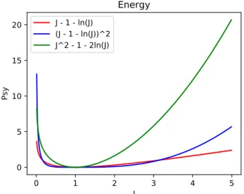
A form of energy for the Mooney-Rivlin model has been choosen, but the bulk energy can have different forms. Here these different forms of energy have been discussed in the following:

(2.73) Ψ1= J − 1 − ln J

(2.74) Ψ2= (J − 1 − ln J)2

(2.75) Ψ3= J2− 1 − 2 ln J

These three different forms of the bulk energy can be shown qualititatively in Figure2.9. All

0

1

2

3

4

5 J

0

5

10

15

20 Psy

Energy

J - 1 - ln(J)

(J - 1 - ln(J))^2

J^2 - 1 - 2ln(J)

Figure 2.9: Three different bulk energy models variation with respect to the compression index

energy form are suitable up to now, as they are all infinity in zero and minimum equal zero when we have no deformation(J = 1) and infinity when J goes to infinity. The first derivative of the bulk energy forms are as the following:

(2.76) ∂Ψ1 ∂J = 1 − 1 J (2.77) ∂Ψ2 ∂J = 2(J − 1 − ln J)(1 − 1 J) (2.78) ∂Ψ3 ∂J = 2(J − 1 J) 20

(34)

1

2

3

4

5 J

4

2

0

2

4

6

8

10 Sigma

Energy_First_derivative

1 - 1/J

(J - 1 - ln(J))(1 - 1/J)

2(J - 1/J)

Figure 2.10: First derivative of three different bulk energy models variation with respect to the compression index

First derivative of these three different forms of the bulk energy can be shown qualititatively in (Figure2.10.)

The first derivative of energy is related to stress. It is evident that for the first energy model, the stress is limited in infinity. It means that there is no solution for stress applied more than the limited value; in other words, “J” is equal to infinity for such stress.

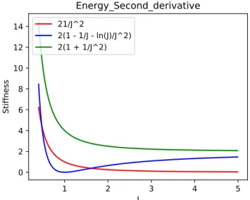
(2.79) ∂ 2_Ψ 1 ∂J2 = 1 J2 (2.80) ∂ 2_Ψ 2 ∂J2 = 2 µ 1 − 1 J− ln J J2 ¶ (2.81) ∂ 2_Ψ 3 ∂J2 = 2 µ 1 + 1 J2 ¶

Second derivative of these three different forms of the bulk energy can be shown qualititatively in (Figure2.11.)

The second energy, which shows the stiffness coefficient, is zero at rest position, which is not proper, and also the first one has the stiffness equal to zero in the infinity, which is not meaningful either.

2.2.3.4 Nonlinearity of the Rivlin Cube

After pulling the Rivlin cube with specific pressure, the minus pressure can be applied to the deformed cube to illustrate the model non-linearity. For example, if the extension with calue

(35)

1

2

3

4

5 J

0

2

4

6

8

10

12

14 Stiffness

Energy_Second_derivative

21/J^2

2(1 - 1/J - ln(J)/J^2)

2(1 + 1/J^2)

Figure 2.11: Second derivative of three different bulk energy models variation with respect to the compression index

of P = 0.2 MPa can be applied in the x-direction to a cube with dimension 10, it leads to the following configuration: (2.82) _{X 1 =}     11.9575926911927 9.58610080999857 9.58610080999857    

And by applying the minus value of the last applied pressure P = −0.2 MPa on the above configuration, it leads to the following configuration:

(2.83) _{X 2 =}     10.6963257156302 9.93319594415821 9.93319594415821    

Which is not the same configuration we started with.

2.3 Inverse Problem

This kind of problem is the most important one is very applicable in biomechanics as there are many problems that the unloaded configuration or material parameter is not known, or it can be the combination of these two. What are know in these kinds of problems are the applied force and some measured deformed configuration. So, it is needed as many data points as the unknown parameters. These parameters can be material parameters or the undeformed configuration, which depends on the coordinates. In the following, all cases of the mentioned materials will be discussed.

(36)

2.3. INVERSE PROBLEM

The golden point which will be presented in the following is that besides the material parameter estimation, only one additional data point is needed for estimation of the unloaded configuration.

2.3.1 Methods for Minimizing a Cost Function

2.3.1.1 Gradient Free Method (CMA)

This method is the least efficient method for finding a minimum for the cost function. It does check different parameters in a specific domain and find the least value of the cost function corresponding to the guessed parameters values. CMA2algorithm has been used for minimizing the cost function by this method.

2.3.1.2 Newton Solver

For the hyperelastic model the stress tensorσ(λ) should be equal to the applied pressure P, but as an initial guess likeλ0 we have a residual which is the difference between the stress tensor

and the applied pressure vector:

(2.84) R0=σ(λ0) − P

In the above equation,σand P are defined as below:

(2.85) σ=     σ11 σ22 σ33     (2.86) _{P =}     P1 P2 P₃     And: (2.87) R0=     σ11− P1 σ22− P2 σ33− P3    

By writing Taylor expansion aroundλ0, the updated law can be obtained.

(2.88) _σ(_λ0+∆λ) ≈σ(λ0) +∂σ

∂λ(λ0) ·∆λ As the following equation exists:

(2.89) σ(λ0+∆λ) = P

(37)

So, the update law would be like Equation (2.90)

(2.90) ∆λ0=

P −σ(λ0)

∂σ

∂λ(λ0)

= −Jac−1· R0

In which Jac is Jacobian matrix of_σ:

(2.91) _{Jac =}∂σ

∂λ

What has been done here is that the cost function should be minimized, which means that its gradient should become zero. So, the Newton method has been done on the derivative of the cost function.

2.3.1.3 Gradient Descent Method

This method is somehow a more straightforward Newton solver, which converges after some steps to the minimum cost function. It can be described as below:

(2.92) x_n+1= xn−γn∇F(xn)

In whichγn can be described as:

(2.93) γn=

¯

¯(xn− xn−1)T[∇F(xn) − ∇F(xn−1)]¯¯ ||∇F(xn) − ∇F(xn−1)||2

In this paperγ0has been considered as 1.

2.3.2 Methods for Computing Gradients and Hessians

So far, different cost functions for the different inverse problems have been suggested, and a common characteristic between them is the convexity of the cost function near the exact value of material parameters or zero with normalized parameters. The existence of a solution for parameters depends on the convexity of the cost function near the solution. So, criteria to chase the behavior of the cost function.

2.3.2.1 Finite difference approximation

The cost function behavior can be predicted by obtaining the gradient or Hessian matrix, and the cost function eigenvalues on the convex point. This can be done numerically and analytically in general. Here it is shown that the gradient of some cost functions numerically can be obtained, with finite difference method.

Two things are calculable here. One is the gradient of the cost function on each point, which is

(38)

applicable for solving the Newton method. Most of the time, the cost function is complicated, that the gradient can not be calculated analytically. So, it is needed to calculate it numerically. The numerical gradient of the cost function J with two parameters in a specified pointθcan be determined below: (2.94) Grad(J(θ)) =   J(h 2,0)−J(−h2,0) h J(0,h 2)−J(0,−h2) h  

An for a cost function with three parameters (like a nonlinear spring) it would be:

(2.95) Grad(J(θ)) =      J(h₂,0,0)−J(−h 2,0,0) h J(0,h₂,0)−J(0,−h 2,0) h J(0,0,h 2)−J(0,0,−h2) h     

One crucial point here is the existence of a minimum for the cost function. The existence of the minimum can be recognized by Hessian matrix. Hessian matrix can be calculated as below:

H( f ) =          ∂2_f ∂x2 1 ∂2_f ∂x1∂x2 · · · ∂ 2_f ∂x1∂xn ∂2_f ∂x2∂x1 ∂ 2_f ∂x2 2 · · · ∂2_f ∂x2∂xn .. . ... . .. ... ∂2_f ∂xn∂x1 ∂ 2_f ∂xn∂x2 · · · ∂ 2_f ∂x2 n         

In which the second derivative would be obtained numerically:

(2.96) ∂

2_f

∂x1∂x2 =

f (h, h) − f (0, h) − f (h,0) + h(0,0)) h2

In which h value supposed a minimal value like 10−6_.

2.3.2.2 The Adjoint Method

The most important thing we need, is the derivative of the cost function- which can be defined as below- with respect to the unknown parameter:

(2.97) J (θ) = Z Ωj(uθ) + β 2||θ−θ0|| 2

In which j(θ) can be as an instant:

(2.98) j(u_θ_{) =}_{¡u − u}mes¢

For obtaining the derivative of the cost function with respect to the parameter we would define the "adjoint problem":

(2.99) J(ˆ _{θ, u) =} Z Ωj(u) + β 2||θ−θ0|| 2

(39)

In which u is supposed independant to_θ. And here Lagrangian is defined as: (2.100) L(θ, u,λ) = ˆJ(θ, u) + Wint(u,λ) − Wext(λ)

By doing the finite differentiation with respect to variables: (2.101) _δ_u_{L · u}∗₌_δ_u_{J · u}ˆ ∗_{+ W}_int(u∗,_{λ) = 0}

(2.102) δ_λL ·λ∗_{= W}int(u,λ∗) − Wext(λ∗) = 0

There is: (2.103) δuL · u∗=δuJ · u∗ As a conclusion: (2.104) L(θ, u,λ) = ˆJ(θ, u) = J(θ) (2.105) ∂J ∂θ ·θ∗= ∂L ∂θ ·θ∗+ ∂L ∂u ∂u ∂θ·θ∗ As a result: (2.106) ∂J ∂θ = ∂L ∂θ(θ, u,λ) 2.3.2.3 Linear Spring

The cost function for solving the inverse problem of the spring can be written as below as mentioned before:

(2.107) _{J(K ) =}1

2¡uK− u

mes¢2

For this simple problem, the derivative of the cost function concerning the material parameter can be obtained easily:

(2.108) ∂J ∂K = ∂J ∂u ∂u ∂K = −(uK− u mes₎ F K2

As in the linear spring u =F_K+ u0. However, by implementing the mentioned method, the

adjoint problem can be defined for that:

(2.109) _{J =}ˆ 1

2¡u − u

mes¢2

So, Lagrangian can be written as:

(2.110) _{L =}1

2¡u − u

mes_{¢ +λ(K (u − u} 0) − F)

(40)

Like the last part, it can be written as below:

(2.111) _δuJ · uˆ ∗= −Wint(u∗,λ)

Which means:

(2.112) _λK u∗_{+ (u − u}mes)u∗_{= 0}

And from the equation (2.102):

(2.113) _{u =}F K+ u0 As a conclusion: (2.114) _λ₌−(u − u mes₎ K

And the derivative of the Lagrangian with respect to the material parameter:

(2.115) ∂L

∂K =λ(u − u0)

So from the equations (2.114) and (2.115) the gradient of the cost function with respect to the material parameter can be obtained:

(2.116) ∂J

∂K =

−(u − umes)F K2

2.3.2.4 Linear Elasticity

The same problem for the linear elasticity problem in continuum mechanics can be solved. In the linear elasticity the Hooke’s law is as below:

(2.117) σ= 2µ²₊λtr(²)I

Here the virtual work of the internal and external forces can be defined as below:

(2.118) Wint(u, u∗) = Z Ω²(u) : C :²(u ∗₎ (2.119) Wext(u∗) = Z ∂ΩF · u ∗ + Z Ωf · u ∗

By assuming Wint= Wextcan obtain the strong form of the equations:

(2.120) d ivσ_{+ f = 0, in}Ω

(41)

(2.122) _σ_{= C :}_²(u), inΩ

For such a material, two material parameters exist, which are_µand_λ. So, two data points are needed: (2.123) J(_µ,_{λ) =} Z Ω 1 2||² µ,λ 1 −² mes 1 || 2 +1 2||² µ,λ 2 −² mes 2 || 2

The adjoint problem can be defined by defining ˆJ (2.124) Jˆi(²) = Z Ω 1 2||²i−² mes i || 2

And Lagrangian is;

(2.125) Li(µ,λ,²,Λ) = ˆJi+ Z Ωσ:²(Λ)− Z ∂ΩF ·Λ− Z ΩfΛ (2.126) Li(µ,λ,²,Λ) = Z Ω 1 2||²i−² mes i || 2 + Z Ωσ:²(Λ)− Z ∂ΩF mes ·Λ− Z Ωf mes_Λ (2.127) δ_²Li·²∗= Z Ω² ∗_||²₋_²mes || + Z Ωσ:² ∗₍_{Λ) = 0}

The above equation is true of every_²∗_{. So:}

(2.128) Z Ω² ∗_||²₋_²mes || = − Z Ωσ:² ∗₍_λ₎ And (2.129) δ_ΛLi·Λ∗= Z Ωσ:²(Λ ∗_{) −}Z ∂ΩF ·Λ ∗₋Z ΩfΛ ∗_{= 0} So: (2.130) Z Ωσ:²(Λ ∗_{) =}Z ∂ΩF ·Λ ∗₊Z ΩfΛ ∗

And derivative of the Lagrangian

(2.131) _δ_λL_i_·_λ∗₌ Z Ωλ ∗³_tr(_²_)I´_² (2.132) _δ_µLi·µ∗= Z Ωµ ∗₍_²₎_² At the end: (2.133) _δ_λ_{J =}_δ_λL1+δλL2 (2.134) δ_µ_{J =}δ_µL1+δµL2 28

(42)

2.3.3 Unloaded Configuration Estimation

2.3.3.1 Linear Spring

Suppose the known parameters are the deformed length of the spring, applied force, and the stiffness coefficient, but the spring undeformed length is unknown. There is one unknown here, and the undeformed length of the spring can be estimated as the following equation:

(2.135) uundef_{= u}d e f₋F E

2.3.3.2 Rivlin Cube

The inverse problem for the Rivlin cube for obtaining the unloaded configuration is such that the applied force and a loaded configuration are known, and the unloaded configuration is the goal. The applied force can be supposed as below:

(2.136) _{F =}     F₁ 0 0 0 F2 0 0 0 F3    

And the deformed configuration is supposed is below:

(2.137) _{X 1 =}     X Y Z    

While X =λ1x, Y =λ2y and Z =λ3z. So, for finding the undeformed configuration x, y and z,

three equations needed to be solved for finding the unloaded configuration:

(2.138) F1=λ1x

(2.139) F2=λ2y

(2.140) F3=λ3z

Saint Venant-Kirchoff is not a good model. To show this fact, the displacement control test was done, and the results, as shown in (Figure2.12) is that when applying the displacement change in the x-direction, the pressure in the x direction is limited. This means that we cannot have any solution for the displacement when we apply a pressure beyond that limit. This shows that the Saint Venant-Kirchhoff model is not good as when the cube is compressed, it will become less stiff, and it would be easier to compress the cube. The other test is applying pressure on the Saint Venant-Kirchhoff Cube in the equitriaxial direction. It means that there is the same pressure in all directions. Another test can be done on this cube, which is controlling the displacement. The λiis changing during this test, and the variation of the pressure is visible in (Figure2.12)

(43)

CHAPTER 2. COMBINED ESTIMATION OF MATERIAL PARAMETERS AND UNLOADED CONFIGURATIONS 0.2 0.4 0.6 0.8 1.0 lambda 3.0 2.5 2.0 1.5 1.0 0.5 0.0 P Px Py Pz (a) Variation of Pi 0.2 0.4 0.6 0.8 1.0 lambda 0.8 0.6 0.4 0.2 0.0 epsilon epsilon_x epsilon_y epsilon_z (b) Variation of²i

Figure 2.12: The variation of the pressure and displacement with respect to the lambda for the compressible Saint Venant-Kirchhoff model

2.3.4 Material Parameter Estimation

There is another kind of problem in which the deformed and undeformed configuration is known while the material property, like the stiffness coefficient here, is unknown, which can be obtained by the Equation (2.141).

(2.141) _{E =} F

ud e f_{− u}undef

This simple problem can be solved by minimizing the cost function as defined in the Equa-tion (2.142). (2.142) _{J(E) =}1 2 ¡ud e f − umes¢2 ¡umes2¢2 umesis what is known from the measurement and:

(2.143) ud e f₌F

E+ u

undef

In Equation (2.143), F and uundef are known. The minimization of this function is done by assuming uundef_{= 0.1 mm, u}d e f_{= 0.2 mm and applied force F = 1 N. This minimization can be} done by hand quickly, but CMA is used here to validate the data. The result of the minimization by CMA is shown in Figure2.13.

Figure2.13 shows the minimization of the cost function for the linear spring for finding the stiffness coefficient. CMA code has done lots of attempts for the given domain to find a minimum for the cost function.

(44)

2.3. INVERSE PROBLEM 8 10 12 14 16 18 20 E 0.000 0.025 0.050 0.075 0.100 0.125 0.150 0.175 J

Figure 2.13: Minimizing the cost function (J(E)) by CMA code for the linear spring.

2.3.4.2 Rivlin Cube

As mentioned in section 2.2.3.1, in the Saint Venant-Kirchhoff model, there are two material parametersλandµ. In solving the inverse problem for the material parameters, it is needed two equations.

An analytical solution is presented when an equitriaxial pressure is applied on the cube with the Saint Venant-Kirchhoff model. In this specific condition:λ1=λ2=λ3=λ0. So, the relation

betweenλand the applied pressure, can be obtained as below:

(2.144) λ₌P +pP

2_{+ (3λ}

0+µ)(3 + 2µ)

(3λ0+µ)

By applying different pressures, the variation ofλwith respect to the applied pressure can be plotted as Figure2.14. For incompressible materialS:

(2.145) Σ =∂Ψ

∂E =λ(trE) + 2µE −γJC

−1

for the incompressible materials, J = 1, so:

(2.146) λ3= 1 λ1λ2 (2.147) σxx= λ2 1[(λ+ 2µ)λ21+λ(λ22+ 1 λ2_1λ2 1) − 3 − 2µ 2 − γ λ2 1 (2.148) _σy y= λ2 2[(λ+ 2µ)λ22+λ(λ21+ 1 λ2_1λ2 2) − 3 − 2µ 2 − γ λ2 2

(45)

5.0 2.5 0.0 2.5 5.0 7.5 10.0 12.5

P

0

2

4

6

8

10 lambda

Figure 2.14: The variation of _λin Saint-Venant Kirchhoff model with respect to the applied equitriaxial pressure applied on Rivlin Cube

4 2 0 2 4 6 P_applied 0.4 0.6 0.8 1.0 1.2 1.4 1.6 1.8 landa landa1 landa2 landa3 (a) Variation ofλi 4 2 0 2 4 6 P_applied 4 2 0 2 4 6 Sigma sigma_x sigma_y sigma_z (b) Variation ofσi

Figure 2.15: The variation of Rivlin cube configuration and stress with respect to applied axial pressure for the incompressible Saint-Venant Kirchhoff model

(2.149) σzz= [(λ+ 2µ) 1 λ2_1λ2 2+λ (λ2₁₊λ2₂) − 3 − 2µ 2λ2₁λ2₂ −γλ 2 1λ22

The previous tests on the compressible material are also done on the incompressible material. The results for the applied force in the x-direction is Figure2.15. For the equitriaxial applied force, the results are as Figure2.16.

There are two unknowns as the parameters of this model, likeµandλ. So, two data points

(46)

2.3. INVERSE PROBLEM 4 2 0 2 4 6 P_applied 0.96 0.98 1.00 1.02 1.04 landa landa1 landa2 landa3 (a) Variation ofλi 4 2 0 2 4 6 P_applied 4 2 0 2 4 6 Sigma sigma_x sigma_y sigma_z (b) Variation ofσi

Figure 2.16: The variation of Rivlin cube configuration and stress with respect to applied equitri-axial pressure for the incompressible Saint-Venant Kirchhoff model

are needed to minimize this cost function.

(2.150) _{J =}1 2 ( £ X1− X₁mes¤2 £ Xmes 1 ¤2 + £ X2− X₂mes¤2 £ Xmes 2 ¤2 )

In which X_imesis the measured configuration, and Xiis the calculated configuration. The problem

here is obtaining the calculated configuration. Supposing the relation below, which was discussed before:

(2.151) σ= (2µ(b − I) + 2λ(ICb − b2− 2I))/J + 2κ(J − 1/J)C−1

As here the matrix C containsλ1,λ2 andλ3, beside the forces applied on the cube, there are

three equations to solve:

(2.152) σx= Px

(2.153) σy= Py

(2.154) σz= Pz

From the above equations,λ1,λ2 andλ3would be obtained with respect toµandλ. So, now

the cost function is only a function ofµandλ, which should be minimized. In section 1.5, it is explained how to minimize the cost function. For the Mooney-Rivlin model, the cost function concerning the dimensionless variables is shown in Figure2.17, and the minimization of each parameter is shown in Figure2.18.

(47)

Normalized mu

0.4 0.2

0.0 0.2

_0.4

Normalized lambda

0.4

0.2

0.0

0.2

0.4 1e31

0.2

0.4

0.6

0.8

1.0

Figure 2.17: Minimization of Mooney-Rivlin cube cost function with respect to re-scaled material parametersλandµ.

2.3.5 Combined Estimation of the Unloaded Configuration and Material Parameters

The more important problem is when the undeformed length or the stiffness of the spring is not known. This problem importance is that because it is a classic problem in biomechanics where the unloaded configuration and the material parameters are unknown most of the time. In this problem, the known data are the deformed configuration and the applied force, but as there are two unknowns: the undeformed configuration and the stiffness coefficient, two sets of data points are needed.

(2.155) E(umes₁ − uund e f) = F1mes

(2.156) E(umes₂ _{− u}_{und e f}_{) = F}₂mes

(48)

2.3. INVERSE PROBLEM 0.2 0.3 0.4 0.5 0.6 0.7 Lmbda 0.0000000 0.0000025 0.0000050 0.0000075 0.0000100 0.0000125 0.0000150 0.0000175 0.0000200 J (a) Variation ofλ 0.4 0.5 0.6 0.7 0.8 Mu 0.000000 0.000002 0.000004 0.000006 0.000008 0.000010 J (b) Variation ofµ

Figure 2.18: Minimization of Mooney-Rivlin cube cost function with respect to re-scaled material parametersλandµ.

From the above equations E and uundefcan be obtained.

(2.157) _{E =}F mes 2 − F mes 1 umes₂ − umes₁ And (2.158) uund e f= u₁mes− F₁mes F₂mes_{− F}₁mes(u mes 2 − u mes 1 )

Now a problem can be defined and solved with two different approaches. Supposing u1= 0.2 mm

and F₁_{= 1 N and another data point as u}₂ _{= 0.22 mm and F}₂_{= 1.2 N, here there are two} equations and two unknowns. With the above equations:

(2.159) _{E = 10}

(2.160) uund e f = 0.1

Of course, this problem is easy enough to be solved by hand, but CMA optimizer can be used for validation such that it minimizes J concerning E and uund e f, which is defined as Equation (2.161).

(2.161) J(E, uund e f) = 1 2 Ã ¡U1− umes₁ ¢2 umes₁ 2 + ¡U2− u₂mes¢2 u₂mes2 ! (2.162) U1= F1 E + uund e f (2.163) U2= F2 E + uund e f

(49)

This cost function can be shown qualitatively as Figure2.19.By having this function in the 3D medium, a good concept can be obtained. The sensitivity of the cost function concerning these parameters is different. So, the cost function is plotted concerning the dimensionless parameters as below: (2.164) J( ˜E, ˜uund e f) = 1 2u2₁ µ_Fmes 1 E + uund e f− u mes 1 ¶ + 1 2u2₂ µ_Fmes 2 E + uund e f− u mes 2 ¶ Such that: (2.165) _{E = (1 + ˜}E) ¯E

(2.166) uund e f= (1 + ˜uund e f) ¯uund e f

The CMA code minimizes the mentioned J concerning the difference between the calculated and measured stiffness coefficient and calculated and measured undeformed length. The result is shown in the Figure2.20

For solving the inverse problem for the material parameter and the unloaded configuration, the cost function has to parameters as Figure2.19. This cost function has a different sensitivity to its variables. The sensitivity can be normalized by changing the variables:

(2.167) _{E = (1 + ˜}E) ¯E

(2.168) uund e f= (1 + ˜uund e f) ¯uund e f

The two-dimensional minimization is shown from each intersection near the minimum configu-ration in Figure2.19and is compared with the results of the CMA code.

2.3.5.2 Rivlin Cube

Here we have the last two unknown parameters plus three new ones like_λ₁,_λ₂, and_λ₃. One data point is needed for estimating the unloaded configuration, and one more is needed for the material parameter estimation as the problem dimension is more than the material problem parameters. So our cost function has five unknowns. The difference between this part and section 1.4.2.2 in which the problem was only the material parameters; here, the cost function has five parameters to minimize. The result of minimization of the cost function with five data points is presented in Figure2.21. In each graph, the cost function minimization is shown concerning the mentioned parameter. (2.169) J =1 2 ( £ X1− X₁mes ¤2 £ Xmes 1 ¤2 + £ X₂_{− X}mes 2 ¤2 £ Xmes 2 ¤2 + £ X3− X₃mes¤2 £ Xmes 3 ¤2 + £ X₄_{− X}mes 4 ¤2 £ Xmes 4 ¤2 + £ X5− X₅mes¤2 £ Xmes 5 ¤2 ) 36

(50)

Normalized Unloaded Length

0.4 0.2

0.0 0.2

_0.4

Normalized Young Modulus

0.4

0.2

0.0

0.2

0.4 J(Cost Function)

0.00

0.07

0.13

0.20

0.27

0.33

0.40

0.46

0.53

0.60

0.1

0.2

0.3

0.4

0.5

Figure 2.19: Linear spring cost function minimization with respect to the re-scaled parameters of the unloaded configuration and Young modulus

2.3.5.3 Tube

For the tube problem, the young modulus exists as the material parameter and the unloaded configuration. There are some time steps, which are the configurations of the tube for different values of the inner pressure. In Figure2.2the first and the last time step has been shown. The tube studied here has a young modulus as its material parameter and n-dimensional coordinates. There are a side of material parameters and an aspect of the unloaded configuration in an inverse problem. For the unloaded configuration, each loaded measured configuration creates as many equations as it is needed to obtain the unloaded configuration.

The material parameter depends on the dimension of the problem. So, suppose the coordinates of the problem are more than the material parameters. In that case, one data point of the measured coordinates creates as many equations as needed to obtain the material parameters.

The unloaded configuration material parameter estimation for the tube has been solved with three different methods. These methods differ in the minimization of the cost function. The first

(51)

CHAPTER 2. COMBINED ESTIMATION OF MATERIAL PARAMETERS AND UNLOADED CONFIGURATIONS 10.0 10.5 11.0 11.5 12.0 12.5 13.0 E 0.0000 0.0002 0.0004 0.0006 0.0008 0.0010 J

(a) Minimization of the cost function with respect to E 0.050 0.075 0.100 0.125 0.150 0.175 0.200 0.225 u_undeformed 0.0 0.5 1.0 1.5 2.0 2.5 3.0 J

(b) Minimization of the cost function with respect to undeformed displacement

Figure 2.20: Minimization of the cost of the linear spring with respect to two parameters of the unloaded configuration and stiffness coefficient

0.40 0.45 0.50 0.55 0.60 0.65 0.70 0.75 lambda 0.00000 0.00025 0.00050 0.00075 0.00100 0.00125 0.00150 0.00175 0.00200 J (a) Variation ofλ 0.40 0.45 0.50 0.55 0.60 0.65 0.70 Mu 0.00000 0.00025 0.00050 0.00075 0.00100 0.00125 0.00150 0.00175 0.00200 J (b) Variation ofµ 9 10 11 12 13 X_undef 0.00000 0.00025 0.00050 0.00075 0.00100 0.00125 0.00150 0.00175 0.00200 J (c) Variation of Xund e f 9.0 9.5 10.0 10.5 11.0 11.5 12.0 12.5 13.0 Y_undef 0.00000 0.00025 0.00050 0.00075 0.00100 0.00125 0.00150 0.00175 0.00200 J (d) Variation of Yund e f 9 10 11 12 13 14 Z_undef 0.00000 0.00025 0.00050 0.00075 0.00100 0.00125 0.00150 0.00175 0.00200 J

(e) Variation of Zund e f

Figure 2.21: Minimization of Mooney-Rivlin cube cost function with respect to re-scaled material parametersλandµand unloaded configuration parameters.

(52)

2.3. INVERSE PROBLEM 8 9 10 11 12 13 14 E 0.000000 0.000005 0.000010 0.000015 0.000020 0.000025 0.000030 J

(a) Cost function

8 9 10 11 12 13 14 E 0.00000 0.00025 0.00050 0.00075 0.00100 0.00125 0.00150 0.00175 Unloaded_cong_err

(b) Unloaded configuration error

Figure 2.22: Tube cost function minimization for the unloaded configuration and material param-eter estimation via CMA code.

6.0 6.5 7.0 7.5 8.0 8.5 9.0 9.5 10.0 E 0.0000 0.0005 0.0010 0.0015 0.0020 0.0025 J

(a) Cost function

6.0 6.5 7.0 7.5 8.0 8.5 9.0 9.5 10.0 E 0.000 0.002 0.004 0.006 0.008 Unloaded_cong_err

(b) Unloaded configuration error

Figure 2.23: Tube cost function minimization for the unloaded configuration and material param-eter estimation via Newton method.

model presented in Figure2.22is the least efficient one. This has been optimized with CMA code, and the minimization takes between 40 to 50 iterations.

Figure2.23and Figure2.24show the Newton solver for minimizing the cost function and Gradi-ent DescGradi-ent solver, respectively. These two methods take almost equal iterations to solve, and both around 10. It is needed to solve the inverse problem for Gradient Descent twice in each iteration and for Newton solver three times. So, the newton solver takes 1.5-time iterations of the Gradient Descent method. Notably, choosing the first step convergence coefficientγ1may also

affect the overall steps.