Thermodynamic Analysis of High Frequency Rectifying Devices: Determination of the Efficiency and Other Performance Parameters

(1)

RESEARCH OUTPUTS / RÉSULTATS DE RECHERCHE

Author(s) - Auteur(s) :

Publication date - Date de publication :

Permanent link - Permalien :

Rights / License - Licence de droit d’auteur :

Dépôt Institutionnel - Portail de la Recherche

researchportal.unamur.be

University of Namur

Thermodynamic Analysis of High Frequency Rectifying Devices: Determination of the Efficiency and Other Performance Parameters

Lerner, Peter B; Miskovsky, Nicholas M; Cutler, Paul H; Mayer, Alexander; Chung, Moon S Published in: Nano Energy DOI: 10.1016/j.nanoen.2012.11.002 Publication date: 2013 Document Version

Early version, also known as pre-print

Link to publication

Citation for pulished version (HARVARD):

Lerner, PB, Miskovsky, NM, Cutler, PH, Mayer, A & Chung, MS 2013, 'Thermodynamic Analysis of High Frequency Rectifying Devices: Determination of the Efficiency and Other Performance Parameters', Nano

Energy, vol. 2, no. 3, pp. 368-376. https://doi.org/10.1016/j.nanoen.2012.11.002

General rights

Copyright and moral rights for the publications made accessible in the public portal are retained by the authors and/or other copyright owners and it is a condition of accessing publications that users recognise and abide by the legal requirements associated with these rights. • Users may download and print one copy of any publication from the public portal for the purpose of private study or research. • You may not further distribute the material or use it for any profit-making activity or commercial gain

• You may freely distribute the URL identifying the publication in the public portal ? Take down policy

If you believe that this document breaches copyright please contact us providing details, and we will remove access to the work immediately and investigate your claim.

(2)

Thermodynamic Analysis of High Frequency Rectifying Devices: Determination

of the Efficiency and Other Performance Parameters

P. B. Lernerb , N. M. Miskovskya,b,*, P. H. Cutlera,b, A. Mayerc , and Moon S. Chungd

a

Scitech Associates, LLC, 232 Woodland Drive, State College, Pennsylvania 16803, USA

b

Department of Physics, 104 Davey Laboratory, The Pennsylvania State University, University Park, Pennsylvania 16802, USA

c

Facultés Universitaires Notre-Dame de la Paix, Rue de Bruxelles 61, 5000 Namur, Belgium

d

Department of Physics, University of Ulsan, Ulsan 680-749, Republic of Korea

Abstract

We derive thermodynamically an expression for the theoretical open circuit voltage of a rectenna device that converts high frequency ac radiation into dc power output. In addition, we obtain the conversion efficiency of an electron emission rectenna, which consists of a nano‐ antenna collector and a geometrically asymmetric rectifying MVM tunnel junction. This quantity plays an analogous role to the fill factor for conventional n‐p semiconducting PV devices in limiting the overall efficiency. Thus, in effect, we develop a theory analogous to the Shockley‐Quiesser Theory or Limit (SHQL) for rectennas. The predicted limitations on the efficiency of the electron emission device, as in the case of the SHQL for n‐p junction devices, are useful for guiding the development of practical devices based on rectennas.[1] These are useful benchmarks for evaluating different electron emission‐based schemes for energy conversion.

1. Introduction

We derive thermodynamically an expression for the theoretical open circuit voltage of a rectenna device that converts high frequency ac radiation into dc power output. In addition, we obtain the conversion efficiency of an electron emission rectenna, which consists of a nano‐ antenna collector and a geometrically asymmetric rectifying MVM tunnel junction. The model device we will consider is a rectenna (an antenna with a rectifier) that converts high frequency ac radiation into dc output power. For a more complete description of this device, and a review of its operation and rectification properties see Reference [2]. The current analysis can be applied to the solar spectrum as well as monochromatic radiation. In an ideal realization, radiation is absorbed by the device that is assumed to be at an equilibrium temperature. A portion of the radiation is reradiated while some is converted into useful work in the creation of an output voltage and power. In evaluating the device performance, we determine the open circuit voltage output, the short‐circuit current, and the energy conversion efficiency.

In the high frequency (optical) range of interest, the quanta in the incident flux are more energetic than those typical for thermal fluctuations in the rectifying antenna, so that the

(3)

2

problem of interaction of the radiation with the material features and, in particular, the tunneling junction, has to be treated quantum mechanically. It is understood that “material features” includes the nano‐dimensions of the structure and tunneling junction. In particular, at optical frequencies (or wavelength about 500 nm or less) the skin depth is on the order of 30 nm, which may coincide with the dimensions of the rectenna, resulting in significant penetration of radiation into the device structure.

The limiting efficiency of the rectifying device cannot, in general, be calculated using a Carnot cycle, which involves only heat exchanges with constant temperature reservoirs because the device is not a heat engine. The second law is, however, still applicable, with entropy changes in the process of energy exchange. When this system is in thermodynamic equilibrium, then, according to the second law of thermodynamics, a fraction of the absorbed power becomes unavailable for work, i.e., conversion to output dc power. For example, photons cannot be absorbed continuously and still have the system maintain a constant temperature. De‐excitation of a fraction of occupied electron states in the absorber must occur to maintain the equilibrium temperature. It is the energy involved in the latter process that is no longer available for conversion into output work (or power).

We now describe qualitatively the processes occurring in such model systems when in thermodynamic equilibrium. Consider radiation incident on a rectifying device (or energy converter). In equilibrium electrons absorb photons and are promoted to excited states, which thermalize to a temperature T0. Assuming the system is in thermal equilibrium at T=T0, the rate

of promotion of electrons must be balanced by radiative de‐excitations. A fraction of the energy of the excited electrons will be converted into electrical energy. Other electrons will give up their energy by either radiative (de‐excitation with photon emission) or through nonradiative thermalization processes, where energy is transferred to the lattice as heat, an irreversible process that generates entropy. In chemical equilibrium with the radiation field the chemical potential energy of the electron gas is equal to that of the emitted photons.[3]

Consider a thermodynamic analysis to determine important parameters of the rectifying device, such as, open‐circuit voltage and efficiency. A flux of photons of frequency ν is incident upon the rectifier. Photons are absorbed and promote electrons to higher energy states in the absorber. To extract electrical energy from the system, there must be a driving force to establish a voltage. An inherent asymmetry in the system can drive the electrons to the interface, thus separating charges and creating an open circuit voltage. The asymmetry can be a junction contact, with a field or density gradient driving the electrons to the interface. The electrons are then delivered during the energy conserving process, such as, elastic tunneling, to the output circuit producing a dc current. This process converts photon energy into a change in electronic potential energy of the system. To determine the open circuit voltage, we analyze this system following the thermodynamical methodology of Markvart.[3,4,5] 2. Calculation of the Voltage under Open Circuit and Dynamic Operating Conditions

(4)

Assume a monochromatic beam of frequency ν is incident upon an ideal rectifier . The internal energy and entropy per photon in the incident beam, uin and sin, respectively, are given

by:[3] ν h u_in = , (1) ⎟⎟ ⎟ ⎠ ⎞ ⎜⎜ ⎜ ⎝ ⎛ + = N c k sin B in

ε

ν 2 2 2 1 ln , (2)

where

ε

inis the étendue (areal expanse) of the incident beam, ν is the frequency of the photon

beam, c is the speed of light, and N the number of photons. The étundue is defined as, θ δ δ δ

ε

₌ 2 _Ωcos A n , (4)

where n is the index of refraction of the medium, ϑ is the angle between the normal to the surface element Aδ and the direction of the photon wave vector k, and Ωδ is the element of solid angle in steradians. For the case of a beam of uniform cross‐sectional area A, the étundue is: A n π

ε

₌ 2 . (5) In Eq. (2), the term ν₂

ε

2 2 c is the number of quantum states within a beam of frequency ν and étundue

ε

. Assume the incident beam impinges upon a rectifying device, where the temperature of the emitted photons is equal to the temperature of the absorber, T0.[6] In general, the energy

spectra of the incident and emitted photon beams are different. For each absorption/emission event some heat (qph) is rejected to the low‐temperature reservoir at temperature T0. This is

accompanied by a change of entropy of 0 T qw . The energy and entropy balance conditions are: w in w q u = + , (6) i w in T q s = −σ 0 , (7)

where σi is the entropy increase during the process of absorption and emission of a single

photon. For the rectifier, the quantity w is the work done in moving a charge through a voltage V from the emitter electrode to the collector electrode. This work is equal to eV, and is, using Eqs. (6) and (7), given by, i in in T s T u eV = − ₀ − ₀σ . (8) Using the relationship,[7] ) ( ) ( ₀ 0 i uin uout T sin sout Tσ = − − − , (9) we obtain, out out T s u eV = − ₀ . (10) Eq. (10) states that the work is equal to the free energy of the emitted photon for a process at constant pressure.[8]

(5)

4

Consider now the entropy changes occurring in the conversion process for an ideal rectifying device, where the absorbed photons are either re‐emitted or their energy transformed into an electrical current. From Ref. [3], σi is given by,

c kin

i σ σ σ

σ = + exp+ , (11)

where σkin represents the entropy changes due to a finite current being extracted from the

device. From Markvart [3], _⎟⎟ ⎠ ⎞ ⎜⎜ ⎝ ⎛ − + + = I I I I I k l l B kin 0 0 ln σ , (12)

with Il , I0, I corresponding to the photogenerated current, the dark saturated current, and

output current, respectively.

The term σexp is the entropy change resulting from the étundue expansion of the

incident beam (i.e., essentially the change in the cross‐sectional area subtended by the incident and emitted photon beams). Markvart[3] calculates this as, ⎟⎟ ⎟ ⎠ ⎞ ⎜⎜ ⎜ ⎝ ⎛ = in out B k

ε

σexp ln . (13) Finally, the term σc is the entropy associated with so‐called “photon cooling.” By this we

mean the after the photon beam is absorbed, the emitted photon beam distribution can be associated with a lower temperature. When the incident photon is cooled to a temperature T0, 1

(

)

( ) 0 out in out in c u u s s T − − − = σ . (14)

To evaluate Eq. (14), we use Eqs. (1)‐ (2) and the following relationships for the emitted photons characterized by temperature T0, uout =hν +kBT₀, (15) ln 0 1 _const. N T k s out out B out + ⎟⎟ ⎟ ⎠ ⎞ ⎜⎜ ⎜ ⎝ ⎛ + ⎟⎟ ⎟ ⎠ ⎞ ⎜⎜ ⎜ ⎝ ⎛ =

ε

_∗ γ , (16)

where Nout is the photon flux rate at temperature T0 and ∗ 2 2 0 2 hc k_Bν γ = , (17) with ν0 the minimum frequency (energy) emitted by the device during the absorption process. In this case, we set ν0=ν, the frequency of the incident radiation, since in this ideal rectifier only radiative transitions are considered. After some algebraic manipulation, we obtain,

(6)

[

]

. 2 ln 2 1 ln 1 ln 2 1 ln ) ( 1 2 2 0 2 2 0 2 2 0 0 ⎥ ⎥ ⎥ ⎦ ⎤ ⎢ ⎢ ⎢ ⎣ ⎡ ⎟ ⎟ ⎟ ⎠ ⎞ ⎜ ⎜ ⎜ ⎝ ⎛ − ⎟⎟ ⎟ ⎠ ⎞ ⎜⎜ ⎜ ⎝ ⎛ + − = ⎥ ⎥ ⎥ ⎦ ⎤ ⎢ ⎢ ⎢ ⎣ ⎡ ⎟⎟ ⎟ ⎠ ⎞ ⎜⎜ ⎜ ⎝ ⎛ + ⎟⎟ ⎟ ⎠ ⎞ ⎜⎜ ⎜ ⎝ ⎛ − ⎟⎟ ⎟ ⎠ ⎞ ⎜⎜ ⎜ ⎝ ⎛ + − + − = ∗ ∗ out B out in out out B in B B c N hc T k N c k N T k N c k T k h h T ν ν γ ν ν ν σ

ε

B . (18) Hence, from Eq. (8), the output voltage is: kin out B out B in out B T N hc T k k T k T h eV ν

ε

ν 0σ 2 2 0 0 0 2 ln ln − ⎟ ⎟ ⎟ ⎠ ⎞ ⎜ ⎜ ⎜ ⎝ ⎛ − ⎟ ⎟ ⎠ ⎞ ⎜ ⎜ ⎝ ⎛ − = _∗ . (19) For the open circuit condition, the final term is zero, and, thus, ⎟ ⎟ ⎟ ⎠ ⎞ ⎜ ⎜ ⎜ ⎝ ⎛ − ⎟ ⎟ ⎠ ⎞ ⎜ ⎜ ⎝ ⎛ − = _∗ out B out B in out B oc N hc T k k T k T h eV 2 2 0 0 0 2 ln ln ν ν

ε

_ε

ε

(20)

The above result does not include non‐radiative losses, i. e., the thermalization of the excited electrons involving the transfer of heat to the lattice. This process is material dependent and irreversible since entropy is generated.

An analogous result for an n‐p semiconducting solar collector assuming the sun is a black body at temperature TS was derived by Markvart in Ref. [3] and is given by: ⎟⎟ ⎠ ⎞ ⎜⎜ ⎝ ⎛ − ⎟⎟ ⎠ ⎞ ⎜⎜ ⎝ ⎛ + ⎟⎟ ⎠ ⎞ ⎜⎜ ⎝ ⎛ − = in out B s B g S oc k T T T T k h T T eV 1 ν ln ₀ln

ε

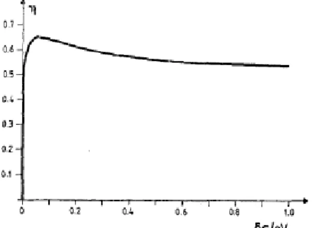
0 0 0 . (21) Eq. (21) reflects the assumption that each photon with an energy above the energy gap yields one electronic charge at a voltage , given by hνg /e=Eg /e, where Eg is the energy gap of

the semiconductor. The result in Eq. (21) also shows that if there is no change in étendue between the incident and emitted beams, the maximum energy output from a system can be specified by the temperatures of the two beams when they originate from bodies in thermal equilibrium at their respective temperatures. For the case treated here of a monochromatic beam incident upon an absorber in thermal equilibrium with its surroundings, the maximum work output is dependent on the temperature of the collector and the energy density of the incident beam, and the étendue (areal expanse) of both the incident and emitted beam, which are no longer equal. Thus, no specific details such as material parameters are needed for the rectifier or the solar absorber. In order to obtain some estimate for the efficiency based upon similar thermodynamic considerations, in Fig. (10) are shown the results from Wurful and Ruppel for the efficiency of conversion for a solar cell, where the incident radiation is absorbed by an intermediate material and re‐emitted over a range of wavelengths corresponding to δε.[9] The maximum efficiency is

(7)

6

about 65% and has a limiting value of 54% as the passband width is increased. These results suggest that high efficiencies compared to the SHQL can be obtained for essentially monochromatic energy sources.

Since the principle of operation of our rectifier is not the same as that in Ref. [9], we analyze and calculate the optimum efficiency for the rectenna device in the next section.

Fig. 1. Efficiency η of ideal thermophotovoltaic energy conversion with a selective intermediate absorber and a solar cell of identical absorption edges at a bandgap of Δεgap = 0.8 eV. The absorber is surrounded by a filter of

passband width δε. The solar radiation is incident onto the absorber with solid angle of Ωinc= 0.03. For δε = 0, no

radiation reaches the solar cell, and η becomes zero. For δε→∞. there is no filtering action, and η approaches the value 0.54 or 54%. [9]

3. Model Calculations of the Limiting Conversion Efficiency of the Rectifying Device

More than half‐a‐century has passed since Shockley and Quiesser developed their much‐celebrated thermodynamic limit on the efficiency of the conversion of solar energy into electricity.[10] While the Shockley‐Quiesser limit (SQL), in many cases, is neither practical nor a real limit (and is not valid when multiphoton processes are significant), the possibility to develop an exact physical constraint on the output work of an electric circuit was a significant achievement in guiding the development of practical power conversion devices using p‐n junction based PV cells. In this section, we establish limitations on the efficiency of rectenna devices using arguments similar to those of Shockley and Quiesser.

We now derive a formula for an optimal power conversion by a model electron emission device based rectenna. This expresses limitations on the maximum efficiency of delivery of output power by the electron emission devices (analogous to the role of the fill factor for determining the efficiency of PV devices).

We shall start with the description of an idealized electron emitter in a rectenna used for the rectification of electromagnetic radiation (see Fig. 2). The determination of the efficiency depends critically on establishing two parameters of importance: the open‐circuit voltage Voc and short‐circuit current Isc. The open circuit voltage Voc is the potential difference

created due to the absorption of radiation under the condition of no current flow. It is given by Eq. (20). The maximum short circuit current Isc is the current produced when every photon

(8)

absorbed is converted to output current. Hence, for a monochromatic incident beam assuming an absorptivity of unity, it is given by: in in sc eN I

ε

• − = , (22) and the power delivered to the “load” is. load load out I V P = (23) Fig. 2 Schematic representation of a generic electron emitter tunnel junction [11] used in the rectenna. The open circuit voltage as given by Eq. (20) or (21) does not depend on the field intensity, only on the energy of the quantum, given by the Einstein relationship. The intuitive meaning of the first term in Eq. (20) or (21) is: an electron is emitted in a single‐photon absorption process of hωopt and transfers its energy to the system when it enters the conduction band of the

anode (reservoir). This energy is divided between potentially useful work and heat losses to the reservoir. The meaning of the logarithmic terms is entropic dissipation of an ordered form of energy (light) into a disordered form (heat). The calculated open circuit voltage would increase if multiphoton absorption in the direction of higher Voc. For simplicity, we retain the unmodified

expression for Voc to emphasize the commonality with the SHQL approach.

In the following analysis, we determine the conditions under which maximum power is delivered to the output circuit, shown below. The energy conversion device can take the place of a battery in the circuit with possible equivalent circuits as shown in Figure 3.

(9)

8

Fig. 3. Possible equivalent circuits for a model rectenna energy conversion device. Choosing the one to use depends on the application, not on an actual circuit design.[12]

We emphasize that an idealized power source with load can be treated as a voltage device (when Théverin equivalent circuit is applicable) as well as a current device (when Mayer‐ Norton equivalent is applicable) dependent on its function. Because the real power source usually falls between a constant voltage and constant current sources, we investigate these two separate cases. The Mayer‐Norton equivalent of a constant current source is more applicable to a rectenna device whose voltage varies considerably with its load. The Thevenin equivalent of a constant voltage source is more applicable to a device in which the current varies, but the applied voltage stays constant. For the device considered here, the voltage output of the rectenna varies with load (so that the Mayer‐Norton Equivalent is more appropriate). However, the Thevenin equivalent circuit provides a second limit to bracket the efficiency because the equivalence of our diode device to one or the other is only approximate. 3.1. Mayer‐Norton treatment assuming the rectenna is a constant current source. Assume the irradiated rectenna is a source of a constant current. A schematic representation of a its diode element in terms of its equivalent circuit is given in Figure 4. Fig. 4 Simplified model of electron emitter rectifier as a constant DC current source.

(10)

Under illumination the device, a voltage is developed across the diode. The operating range of the device is between 0 and Voc with output power delivered to the load given by, V I P_out = ⋅ , (23) with the assumption that the dark current of the diode under a bias V is given by the Fowler‐ Nordheim (FN) formula, ⎟ ⎠ ⎞ ⎜ ⎝ ⎛ − Κ = V V Idark α exp 2 _, ₍₂₄₎ where Κ=SA and α =Bφ3/2. Here, Eq. (23) is simply Joule’s law where I is the current delivered to the load and V is the output voltage. When a load is present, a potential develops between the terminals of the diode, creating a current, Idark, through the diode that opposes ISC. Hence, the current delivered

to the external load is given by ISC – Idark. This so‐called dark current is the current delivered by

the diode under a bias equal to V.

Eq. (24) is a Fowler‐Nordheim type equation, where A and B are the usual FN parameters, S is the emitting surface area, . The quantity r0 is the average radius

of curvature of the emitting element, Δθ≈arctan(h/L) is the effective emitting angle, and N is the total number of emitters per unit area.[

N r

S ≈π 02Δθ⋅

13,14] Note, that the canonical FN equation deals with the current density, whereas, Equation (24) is the expression for the total current as required by the Joule law.

There is no contradiction between Equation (20), which assumes single‐photon processes and Equation (24), which is based on Fowler‐Nordheim approach. The FN law can be understood in terms of multi‐photon absorption and corresponds to the limit when the number of photons absorbed. nph→∞.[15] Using the approach governing the derivation of the

Schokley‐Quiesser formula, we assume that the energy of an optical photon is completely absorbed in the device and, thereby, fully converted into the energy of electrons and the crystalline lattice. The useful work produced by the device has an optimum value at a particular load impedance. The maximum power output is obtained by choosing the voltage so that the product IV is maximized. Using Eq. (24), the short circuit current is, ⎟⎟ ⎠ ⎞ ⎜⎜ ⎝ ⎛ − Κ = OC OC SC V V I 2exp α . (25) The power output delivered to the load is, V V KV V V V I I P OC OC dark SC out ⎟⎟ ⎠ ⎞ ⎜ ⎜ ⎝ ⎛ ⎟ ⎠ ⎞ ⎜ ⎝ ⎛ − − ⎟⎟ ⎠ ⎞ ⎜⎜ ⎝ ⎛ − Κ = − =( ) 2exp α 2exp α (26) Using the following dimensionless quantities. OC V V x= , with 0≤ x≤1, (27)

(11)

10 OC V b= α , (28) 3 OC out norm KV P P = ’ (29)

the normalized power output Pnorm is given by,

( )

(

)

(

b x b x

)

x

P_norm = exp − − 2exp − / . (30)

Note that the dimensionless parameter appearing in the exponential of the FN equation is a measure of the transparency of the barrier for electron tunneling and can also be expressed as, OC OC F V b 2 / 3 693 . 0 φ α = = , (31)

where FOC is the field at the cathode (in V/Å) under an applied voltage of VOC and ɸ is the work

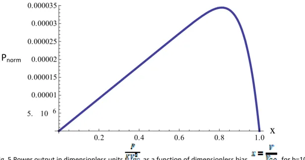
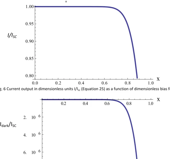
function (in eV). In the ordinary electron (field) emission range, the field is of the order of 0.3 to 0.7 V/Å, with ɸ of the order of 4 eV for most metals. Hence, b for an electron emitter in the ordinary field emission range ranges between 8 and 18. The characteristic dependence of output power, current and dark current as a function of x for b=10 is given in Figsures 5‐7, respectively. These qualitatively resemble the characteristics of an ideal p‐n junction device. 0.2 0.4 0.6 0.8 1.0

x

5. 10 6 0.00001 0.000015 0.00002 0.000025 0.00003 0.000035

P

norm

(12)

0.0 0.2 0.4 0.6 0.8 1.0

x

0.80 0.85 0.90 0.95 1.00

e s o ess Cu e Ou pu

I/I

SC Fig. 6 Current output in dimensionless units I/Isc (Equation 25) as a function of dimensionless bias for b=10. 0.2 0.4 0.6 0.8 1.0

x

6. 10 6 4. 10 6 2. 10 6

I

dark

/I

SC

Fig. 7 Variation of a dark current Idark/Isc as a function of bias for b=10.

In order to determine the optimal value of the output power as a function of x, we use the following condition: 0 = dx dP_norm . (32) It is important to note that the output power depends upon the device’s physical and geometrical parameters that are embedded in the constant b. Hence, for a practical device, the optimization of the device requires the appropriate choice of device parameters.

To calculate the conversion efficiency at maximum power (analogous to the fill factor (FF)), we use the following expression, m m V I V I = η , (33)

(13)

12

which is the maximum power delivered to the load divided by the input power supplied by the flux of quanta, neglecting small corrections of the order kBT0. The following plot shows its

dependence on b. The limiting value is 1 as b increases. 10 20 30 40 50 60 70

b

0.2 0.4 0.6 0.8

η

Fig. 9 Efficiency η as a function of b, the transparency of the barrier. Note that for moderately transparent barriers (b~10), the efficiency is greater than 70%. 3.2. Thevenin treatment assuming the rectenna is a constant voltage source Fig. 10. Schematic diagram of a circuit with a rectenna under illumination, including the antenna, the rectifying element and the load.

(14)

In order to determine the optimal value of the output power delivered to the load for the circuit shown in Fig. 10, we use the method of Lagrange multipliers (see the Appendix). The optimal value of the output voltage delivered to the load is: 6 12 ) 4 ( ) 4 ( 2 2 oc oc oc opt load V V V V = +α ± +α − (34) The parameter α is a device‐dependent material and geometric quantity. The power delivered to the load is, opt load opt out I V P = . (35) The total energy delivered by the “battery” is, e I V I

P_tot = _opt _oc ≈ _opt hω (36)

Using Eqs. (35) and (36), we obtain for the efficiency (energy conversion coefficient):

( )

ω η h opt load eV = (37)

Neglecting small corrections of the order kBT0 to Voc, the efficiency is calculated as a function of

frequency. The results of the calculations are shown in figures 11 and 12 for a model device characterized by the following parameters: ɸ=4.5 eV, s=1 nm, and β=20. In addition, for this idealized case, we assume the time scale for tunneling is much shorter than that associated with thermalization processes.

0.2

0.4

0.6

0.8

1.0

0.05

0.10

0.15

0.20

0.25 η

λ’

Fig. 11. The efficiency of energy conversion, η, as a function of a dimensionless wavelength defined by λ’=λφ/2πch. Note that the efficiency increases monotonically with the energy of a photon until it is approximately constant from the near IR (about 1eV) through the visible, the peak region of the curve.

The results suggest that the efficiency of rectification of the optical radiation by the rectenna treated as a constant voltage source is comparable to the SHQL but not as high as in a Mayer‐

(15)

14

Norton model. Specifically, the value of the conversion efficiency asymptotically approaches η= . Moreover, the efficiency integrated over a Planck integrated solar spectrum is even lower, with η<30%. 4. Summary and Conclusions In this paper we derive a thermodynamic expression for the theoretical open circuit voltage of an electron emission device (rectenna) that converts high frequency ac radiation into dc power output. In addition, we derive expressions for the conversion efficiency, i.e., the efficiency of delivery of output power to a load and its dependence on physical constants and geometrical factors.

The conversion efficiency plays a role analogous to the fill factor (for PV devices) in limiting the overall efficiency. The energy harvesting device treated here is a rectenna with a rectifying element consisting of a geometrically asymmetric tunnel junction. The rectification process of this rectenna is based, not on conventional material or temperature asymmetry as used in MIM (Metal/Insulator/Metal) or Schottky diodes, but on a purely geometric property of the antenna tip or other sharp edges that may be incorporated on antennas. This “tip” or edge in conjunction with a collector anode provides a connection to the external circuit and constitutes a tunnel junction. In these devices the rectenna (consisting of the antenna and the tunnel junction) acts as both the absorber of the incident radiation and the rectifier. Using current nanofabrication techniques and the selective Atomic Layer Deposition (ALD) process, junctions on the order of 1 nm can be fabricated, which allow for rectification of frequencies up to the blue portion of the spectrum.

In treating a solar cell or more general solar energy harvester as the electrical energy source in a circuit, there are two limiting cases: The circuit can be modeled as voltage source whose emf is essentially independent of the load resistance; The circuit can be modeled as a constant current source whose emf depends on the load resistance. A choice of one or the other depends on the particular application.

In the conventional analysis of the efficiency of a solar cell (i.e., single n‐p junction), the device is treated as a constant current source. In this case, the energy efficiency is expressed in terms of the short circuit current (load resistance is 0) and the open circuit voltage (load resistance is ∞) and the fill factor. For our rectenna, the device is more accurately treated as a current source because the output emf depends on the resistance of external load, with the operating voltage of the device varying between 0 and Voc. Calculated results indicate that

within this context, the efficiency of conversion of monochromatic light can exceed η=70%, with correspondingly high integrated efficiencies over the solar spectrum.

By contrast, if we treat the rectennas as a constant voltage (emf) source, the current fluctuates dependent on the load. In this case, the device operates at a voltage V≈Voc and the

maximum theoretical efficiency is much lower, asymptotically approaching η= . The efficiency integrated over a Planck integrated solar spectrum is even lower, with η<30%.

(16)

In conclusion, the treatment presented here complements Shockley‐Quiesser theory when the solar energy harvesting device is a rectenna rather than a p‐n junction for conversion into electrical energy. It is based only on the Second Law of Thermodynamics and Joule’s law. Given that the rectenna device corresponds more closely in a equivalent circuit approach to a constant current rather than constant emf source, efficiencies much greater than 30% can be expected, on the order of 70%, for an optimized device. These higher efficiencies can be further enhanced by the inclusion of multiphoton absorption processes. The calculated results provide a new benchmark for the limiting efficiency of rectennas in the frequency range from the IR to the near ultraviolet. Acknowledgement We thank Dr. Thomas A. Sullivan (Department of Electrical & Computer Engineering, Temple University, Philadelphia, Pennsylvania 19122, USA) for his useful review and critique.

(17)

16 Appendix. Derivation of the Optimal Power Output in the Constant Voltage Regime Using the Method of Lagrange Multipliers, we find the optimal value of the output power r I P_out = 2 , (A.1) subject to the constraint that the current is given by the FN formula, ⎟⎟ ⎠ ⎞ ⎜⎜ ⎝ ⎛ − − − Κ = ) ( exp ) ( 2 Ir V Ir V I oc oc α , (A.2) Where the notation is discussed following Eq. (24). With λ denoting the Lagrange multiplier, the operational relationship for the Lagrange method is given by. 0 ] [ ) ( exp ) ( 2 2 ₌ ₋ ₌ ⎥ ⎥ ⎦ ⎤ ⎢ ⎢ ⎣ ⎡ ⎭ ⎬ ⎫ ⎩ ⎨ ⎧ ⎟⎟ ⎠ ⎞ ⎜⎜ ⎝ ⎛ − − − Κ − − f g Ir V Ir V I r I oc oc δ λ α λ δ . (A.3) This reduces to the following three equations, 0 ) ( = ∂ − ∂ I g f λ (A.4) 0 ) ( ₌ ∂ − ∂ r g f λ (A.5) 0 ) ( ₌ ∂ − ∂ λ λg f (A.6) Evaluating Eq. (A.4) yields, 0 ) ( exp ) ( ) ( ) ( ) ( exp ) )( ( 2 1 2 2 ₂ ₌ ⎭ ⎬ ⎫ ⎩ ⎨ ⎧ ⎟⎟ ⎠ ⎞ ⎜⎜ ⎝ ⎛ − − − − − Κ − ⎟⎟ ⎠ ⎞ ⎜⎜ ⎝ ⎛ − − − − Κ − − Ir V r Ir V Ir V Ir V r Ir V Ir oc oc oc oc α α α λ Simplifying,

(18)

0 ) ( exp ) ( exp ) ( 2 1 2 = ⎭ ⎬ ⎫ ⎩ ⎨ ⎧ ⎟⎟ ⎠ ⎞ ⎜⎜ ⎝ ⎛ − − Κ + ⎟⎟ ⎠ ⎞ ⎜⎜ ⎝ ⎛ − − − Κ + − Ir V r Ir V Ir V r Ir oc oc oc α α α λ (A.7) and using the constraint, yields,

{

( ) 2 ( )

}

0 ) ( 2 ₋ 2₋ ₋ 2₊ ₋ ₊ ₌ rI Ir V rI Ir V Ir V Ir _oc λ _oc _oc α (A.8) Evaluating Eq. (A.5), yields, 0 ) ( exp ) ( ) ( ) ( ) ( exp ) )( ( 2 2 ₂ 2 ₌ ⎭ ⎬ ⎫ ⎩ ⎨ ⎧ ⎟⎟ ⎠ ⎞ ⎜⎜ ⎝ ⎛ − − − − − Κ − ⎟⎟ ⎠ ⎞ ⎜⎜ ⎝ ⎛ − − − − Κ − − Ir V I Ir V Ir V Ir V I Ir V I oc oc oc oc α α α λ Dividing by I and simplifying, 0 ) ( exp ) ( exp ) ( 2 = ⎭ ⎬ ⎫ ⎩ ⎨ ⎧ ⎟⎟ ⎠ ⎞ ⎜⎜ ⎝ ⎛ − − Κ + ⎟⎟ ⎠ ⎞ ⎜⎜ ⎝ ⎛ − − − Κ − Ir V Ir V Ir V I oc oc oc α α α λ Using the constraint and further simplification, we obtain, ( ₋ )2₋_λ

{

2( ₋ )₊_α ₌0 (A.9) Ir V Ir V_oc _oc

}

The final condition, Eq. (A.6), just reiterates the constraint on the FN current, 0 ) ( exp ) ( 2 ₌ ⎭ ⎬ ⎫ ⎩ ⎨ ⎧ ⎟⎟ ⎠ ⎞ ⎜⎜ ⎝ ⎛ − − − Κ − Ir V Ir V I oc oc α (A.10) Solving for λ in both Eq. (A.8) and Eq. (A.9) and equating the results yields, α α − + − = + − + − − ) ( 2 ) ( ) ( 2 ) ( ) ( 2 2 2 2 Ir V Ir V rI Ir V rI Ir V Ir V Ir oc oc oc oc oc . (A.11) Letting y=Ir, expanding terms and simplifying yields the following quadratic equation in y, 3 2₋(4 ₊ ) ₊ 2 ₌0. (A.12) oc oc y V V y α The solution of the quadratic equation is, 6 12 ) 4 ( ) 4 ( 2 2 oc oc oc V V V y= +α ± +α − . (A.13)

(19)

18

Using the dimensionless units x, b, and Pnorm defined in Eqs. (27)‐(29), we obtain,

6 12 ) 4 ( ) 4 ( ₊ _± ₊ 2₋ = b b x , (A.17) which is the fraction of the output voltage of the source across the load.

(20)

[1] G. S. Crabtree and N. S. Lewis, “Solar Energy Conversion” in Physics Today, March 2007, 60(3), 38‐42. [2] Nicholas M. Miskovsky, Paul H. Cutler, A. Mayer, Brock L. Weiss, Brian Willis, Thomas E. Sullivan, and Peter B. Lerner, “Nanoscale Devices For Rectification Of High Frequency Radiation From The Infrared Through The Visible: A New Approach,” Journal of Nanotechnology, in press (2012). [3] T. Markvart, “COUNTING SUNRAYS: FROM OPTICS TO THE THERMODYNAMICS OF LIGHT,” in Physics of the Nanostructured Solar Cells, edited by Badescu, V. and M. Paulescu, Nova Science Publishers, New York, USA (2009). [4] T. Markvart, “Thermodynamics of losses in photovoltaic conversion,” Appl. Phys. Lett. 91, 064102 (2007). [5] T. Markvart, “Solar cell as a heat engine: energy‐entropy analysis of photovoltaic conversion,” Phys. Stat. Solidi (a) 205, no. 12, 2752 (2008). [6] This temperature should be characteristic of the electronic degrees of freedom. [7] As pointed out by Markvart in Ref. [3], the entropy generation per photon, σi, represents the absorbed and emitted photons at constant volume. [8] A. B. Pippard, The Elements of Classical Thermodynamics, Cambridge University Press (1964). [9] P. Wurfel and W. Ruppel, “Upper Limit of Thermovoltaic Solar Energy Conversion,” IEEE Trans. on Electron. Devices 27, 745 (1980). [10] William Shockley and Hans J. Queisser, “Detailed Balance Limit of Efficiency of p‐n Junction Solar Cells,” J. Appl. Phys. 32, 510 (1961). [11] C. A. Spindt, "A thin‐film field‐emission cathode", Journal of Applied Physics, vol. 39, no. 7, pages 3504‐3505, 1968, U.S. Patent 3,755,704 granted on August 28, 1973. [12] http:/cnx.org/content/m0020/latest/ [13]Murphy, E. L. and Good, R. H., 1956, “Thermionic emission, field emission and the transmission region,” Phys. Rev., 1956, 102, 1464‐1473. [14] P. H. Cutler, N. M. Miskovsky, P. B. Lerner and Moon S. Chung, “The use of internal field emission: a review,” Applied Surface Science, 146, 123 (1999). [15] M.V. Ammosov, N.B. Delone, and V.P. Krainov, Zh. Eksp. Teor. Fiz. 91, 2008 (1986) [Sov. Phys. JETP 64, 1191 (1986)].