HAL Id: tel-03207261
https://tel.archives-ouvertes.fr/tel-03207261
Submitted on 24 Apr 2021HAL is a multi-disciplinary open access archive for the deposit and dissemination of sci-entific research documents, whether they are pub-lished or not. The documents may come from teaching and research institutions in France or abroad, or from public or private research centers.
L’archive ouverte pluridisciplinaire HAL, est destinée au dépôt et à la diffusion de documents scientifiques de niveau recherche, publiés ou non, émanant des établissements d’enseignement et de recherche français ou étrangers, des laboratoires publics ou privés.
Characterization, evaluation and utilization of clock
jitter as source of randomness in data security
Elie Noumon Allini
To cite this version:
Elie Noumon Allini. Characterization, evaluation and utilization of clock jitter as source of randomness in data security. Cryptography and Security [cs.CR]. Université de Lyon, 2020. English. �NNT : 2020LYSES019�. �tel-03207261�
T
HÈSE
de D
OCTORAT DE L
’U
NIVERSITÉ DE
L
YON
opéré au sein duLaboratoire Hubert Curien
Ecole DoctoraleN◦488 Sciences Ingénierie Santé
Spécialité: Informatique
Soutenue publiquement le 14 Septembre 2020 par : Elie Noumon Allini
Caractérisation, évaluation et utilisation du jitter d’horloge comme source
d’aléa dans la sécurité des données
Devant le jury composé de :
Bossuet, Lilian Professeur Université Jean Monnet Président Dutertre, Jean-Max Professeur École des Mines de Saint-Étienne Rapporteur Elbaz-Vincent, Philippe Professeur Université Grenoble-Alpes Rapporteur Fontaine, Caroline Directrice de Recherche CNRS / ENS Paris-Saclay Examinatrice Lubicz, David Ingénieur de Recherche DGA-MI / Université Rennes 1 Examinateur Fischer, Viktor Professeur Université Jean Monnet Directeur de thèse Bernard, Florent Maître de Conférences Université Jean Monnet Co-encadrant de thèse
P
H
D
THESIS
from U
NIVERSITÉ DE
L
YON
carried out atLaboratoire Hubert Curien
Doctoral schoolN◦488 Sciences Engineering Health
Speciality: Computer Science
publicly defended on September 14th, 2020 by:
Elie Noumon Allini
Characterization, evaluation and utilization of clock jitter as source of
randomness in data security
In front of the jury consisting of:
Bossuet, Lilian Professor Université Jean Monnet President Dutertre, Jean-Max Professor École des Mines de Saint-Étienne Reviewer Elbaz-Vincent, Philippe Professor Université Grenoble-Alpes Reviewer Fontaine, Caroline Senior Researcher CNRS / ENS Paris-Saclay Examiner Lubicz, David Research Engineer DGA-MI / Université Rennes 1 Examiner Fischer, Viktor Professor Université Jean Monnet Supervisor Bernard, Florent Associate Professor Université Jean Monnet Co-supervisor
Générale de l’Armement under grant agreement No 16810066.
Acknowledgements
This PhD was an enriching experience, on a personal, scientific and human dimension. I consider myself extremely privileged to have been able to carry out this experience in company of extraor-dinary people. I give thanks to God, the Father of my Lord Jesus Christ for this tremendous grace he has granted me.
To Viktor Fischer and Florent Bernard, I owe a big thanks for the confidence they have placed in me. I am very grateful to have benefited from their guidance during these years of doctoral stud-ies. With them, I discovered new scientific disciplines, allowing me to increase my perspective. Their availability, their expertise have brought me a lot during these years. Their rigor pushed me beyond my limits, allowing me to improve enormously.
My gratitude also goes to DGA for the funding of my PhD thesis. My special thanks to David Lubicz who associated me with this certification work that is so important to DGA. Thank you David for your comments and questions that have greatly contributed to the quality of my work. Many thanks to Jean-Max Dutertre and Philippe Elbaz-Vincent for reporting my work. The ex-cellence of their remarks and comments reflects the time and care given to my work despite the difficulties related to the health crisis of Covid-19. I would also like to thank Lilian Bossuet for the wonderful welcome within the SESAM team. Thanks to this, I have been able to work serenely during these three years and devote myself exclusively to my PhD.
I would also like to thank Caroline Fontaine who introduced me to the world of research, thanks to my master’s internship that she directed, she helped me open a path that led me to this PhD. Her advice and support went beyond my internship and was beneficial to me during my doctoral experience.
The major difficulty (and also the beauty) of this thesis is that it required expertise in so many fields that I lost count. I don’t consider myself an expert in these fields, I had the grace of
bene-fiting from the expertise of the greats in these fields. Among these experts, I can name François Vernotte and Enrico Rubiola who helped me enormously to understand frequency stability. Chap-ter2of this thesis attests of their availability and the enriching discussions I had with them. You have my full acknowledgement.
My heartfelt thanks to Jean-Jacques Rousseau, who helped me enormously to get up to speed in electronics and automation. Our recurring discussions have given me a better understanding of this world that was entirely new to me. Thanks to this, I was able to understand better how filters and PLL work. It is therefore obvious that you played an important part in the success of my thesis. Many thanks to you JJR.
I would like to thank all the members of the SESAM team in which I carried out my thesis work. The good attitude and availability of each of its members contributed to a healthy working envi-ronment. Special thanks to Nathalie Bochard for her help with the electronic aspects, as well as for her dynamism. I was honored to share the same office with Brice Colombier, Ugo Murredu and Oto Petura. I hope I didn’t traumatize them with my endless equations on the board. I will miss the atmosphere in this office and our discussions.
I also thank Alain Aubert, Pierre-Louis Cayrel and Vincent Grosso for their simplicity. A special mention to El Mehdi Benhani, our TrustZone expert, who started his PhD and completed it al-most at the same time as me. I wish you a very good career, and by the way, a happy marriage. I do not forget of course to Damien Robissout and Gabriel Zaïd (affectionately Titi) the experts of the team in Deep Learning and side channel and wish them a good completion of their PhD. My gratitude also goes to my family, who have been an unfailing source of support. Your encour-agement, advice and constant presence have been crucial to the success of this thesis and I am deeply grateful for that.
I also thank Julia Leute, Olivier Marchal, and many others. They were so numerous to have contributed to the success of this PhD. Many thanks to all of you and may God bless you endlessly.
Contents
Acknowledgements 1
Introduction 1
Objectives . . . 3
Objectifs de la thèse . . . 6
1 Random numbers in cryptography: state-of-the-art 9 1.1 Random number generators . . . 10
1.1.1 Pseudorandom number generators . . . 10
1.1.2 True random number generators . . . 14
1.1.2.1 Source of randomness. . . 15
1.1.2.2 Randomness harvester . . . 16
1.1.2.3 Post-processor . . . 16
1.2 Sources of randomness in logic devices . . . 17
1.2.1 Commonly used sources of randomness . . . 18
1.2.2 Clock jitter as a source of randomness . . . 18
1.2.2.1 Absolute jitter . . . 19 1.2.2.2 Relative jitter . . . 20 1.2.2.3 Period jitter. . . 21 1.2.2.4 N-Period jitter . . . 22 1.2.3 Jitter sources . . . 24 1.3 Entropy. . . 26 1.3.1 Rényi entropy . . . 26 1.3.1.1 Understanding entropy. . . 26
1.3.1.2 General properties of Rényi entropy . . . 27
1.3.2 Shannon entropy . . . 29
1.3.2.1 Conditional entropy - Mutual information . . . 29
1.4 Evaluation of TRNGs . . . 31
1.4.1 Classical evaluation approach of TRNGs . . . 35
1.4.2 Enhanced evaluation approach of TRNGs . . . 37
1.5 Conclusion . . . 41
2 Characterization of clock jitter as a source of randomness 45 2.1 Random signal . . . 46
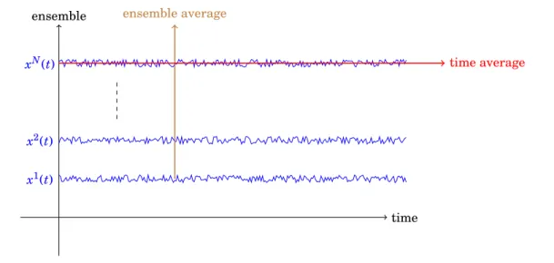
2.1.1 Time and ensemble averages. . . 46
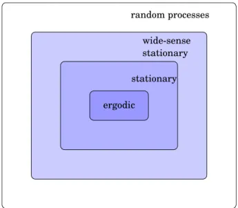
2.1.2 Classification of random processes . . . 48
2.1.2.1 Continuous processes . . . 48
2.1.2.2 Deterministic processes . . . 48
2.1.2.3 Stationarity . . . 49
2.1.2.4 Ergodicity. . . 50
2.2 Mathematical model of the clock jitter . . . 50
2.2.1 Characterizing noise in time domain . . . 51
2.2.1.1 Oscillator output signal . . . 51
2.2.1.2 Phase and frequency random fluctuations . . . 54
2.2.1.3 Average fractional frequency . . . 55
2.2.1.4 Limitations of the model . . . 56
2.2.1.5 Autorrelation function . . . 57
2.2.2 Characterizing noise in frequency domain. . . 58
2.2.2.1 Power spectral density . . . 59
2.2.2.2 Wiener-Khinchin theorem . . . 61
2.2.2.3 Relationships between power spectral densities . . . 62
2.2.3 Noise models . . . 63
2.2.3.1 White noise . . . 63
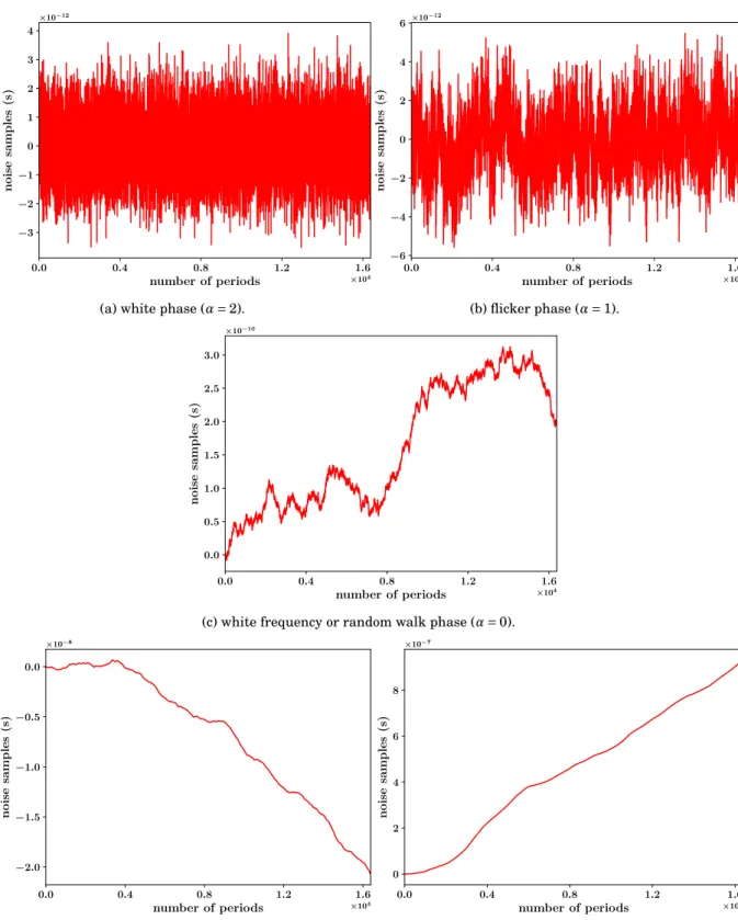
2.2.3.2 Power law noise . . . 65
2.2.3.3 Noise simulation. . . 66
2.3 Jitter analysis tools . . . 67
2.3.1 Limitation of the classical variance . . . 67
2.3.2 Allan variance . . . 70
2.3.2.1 Description of the Allan variance . . . 70
2.3.2.2 Overlapped Allan variance . . . 71
2.3.2.3 Application to noise identification . . . 72
2.3.3 Modified and time versions of the Allan variance . . . 73
2.3.3.2 Time Allan variance . . . 75
2.3.4 Noise identification using autocorrelation function . . . 77
2.4 Jitter measurement method . . . 79
2.4.1 Counter based method for jitter measurement . . . 79
2.4.2 Jitter measurement in hardware . . . 81
2.5 Estimation of the thermal noise contribution . . . 83
2.6 Conclusion . . . 88
3 Phase-locked loops as sources of randomness 91 3.1 Phase-locked loops . . . 92
3.1.1 Basic PLL overview . . . 92
3.1.2 Basic equations of the PLL . . . 93
3.1.2.1 Basic PLL transfer functions . . . 93
3.2 Transfer functions of an analog PLL . . . 95
3.2.1 Open loop transfer function . . . 95
3.2.2 Closed loop transfer function. . . 96
3.2.3 PLL in presence of disturbing signals . . . 96
3.3 Physical parameters of the PLL model . . . 99
3.3.1 Comparison with existing models . . . 99
3.3.2 Choice of physical parameters . . . 100
3.4 Noise properties . . . 102
3.4.1 Origin of the output noise . . . 102
3.4.2 Noise filtering and jitter overshoot . . . 104
3.4.2.1 Jitter peaking . . . 105
3.4.2.2 PLL response to input noise . . . 105
3.4.2.3 PLL response to VCO noise . . . 107
3.4.2.4 Lowering the jitter peaking . . . 108
3.4.3 Types of noise at the output of the PLL . . . 110
3.4.4 Bounded nature of the PLL noise . . . 110
3.5 Conclusion . . . 112
4 Design of a certifiable PLL-based TRNG 115 4.1 Principle of a PLL-based TRNG . . . 116
4.2 Illustration of the DGA-MI approach on PLL-based TRNG . . . 120
4.2.1 Entities of a generator . . . 121
4.2.1.1 Physical noise source . . . 121
4.2.1.3 Post-processing block . . . 122
4.2.1.4 Embedded tests . . . 122
4.2.2 Evaluation of the physical noise source . . . 123
4.2.3 Evaluation of the randomness harvester. . . 126
4.3 Optimal configurations for a PLL-based TRNG . . . 127
4.3.1 Statement of the problem. . . 128
4.3.1.1 General structure of the PLL and its configuration . . . 128
4.3.1.2 Problem to solve . . . 130
4.3.2 Search of PLL-TRNG configurations . . . 131
4.3.2.1 Search of all feasible configurations . . . 132
4.3.2.2 Search of suitable configurations . . . 133
4.3.3 Experimental results . . . 134
4.3.3.1 Implementation considerations . . . 134
4.3.3.2 Results and discussions . . . 136
4.3.3.3 Comparison with the previous method . . . 137
4.4 Conclusion . . . 138 Contributions 143 Conclusion 147 Perspectives . . . 150 Perspectives à la thèse. . . 154 List of Figures i List of Tables iii References v A LTI and random processes 1 A.1 Introduction to linear time-invariant systems. . . 1
A.2 Response of LTI to random input . . . 2
A.2.1 Analysis in the time domain . . . 2
A.2.1.1 Expected value of y . . . 3
A.2.1.2 Mean-square value of y. . . 3
A.2.1.3 Autocorrelation function of y . . . 4
A.2.2 Analysis in the frequency domain . . . 4
C.1 Allan variance generalizes the classical variance. . . 9 C.2 Multiplication by a scalar . . . 10 C.3 Sum of independent random processes . . . 10
Introduction
Throughout history, information has proved itself to be an increasingly valuable asset. From it depended government decisions, military actions, business prospects and so much more [1]. This reflects the essential importance of information and, at the same time, shows how important it is to protect it. A common way of protecting information is cryptography [2,3]. Indeed, by encrypt-ing the information, it becomes inaccessible to any unauthorized party. The encryption process involves mathematical algorithms for which prime numbers are very important [3, Chapter 4]. However, there is a second class of numbers almost as important as prime numbers, namely ran-dom numbers [4,5,6].
Modern cryptography is based on a set of fundamental principles, one of which is the Kerckhoff Principles, which stipulate, among other things, that the security of any cryptographic construc-tion must not be compromised even if everything related to that construcconstruc-tion is made public, except the key [7]. This implies that the security of any cryptographic construction must be based solely on secret keys, and thus imposes high requirements on them. It is therefore understood that a cryptographic key can under no circumstances be exported outside the cryptosystem in clear. It is also essential that it is stored in a secure area to prevent unauthorized access to this key. However, protecting access to this key would be useless if an adversary can easily guess it. These keys have to be, in addition, unpredictable. This unpredictability is only accessible through random numbers, which are unpredictable in nature. We therefore need a process to generate ran-dom numbers, such a process is known as a ranran-dom number generator (RNGs) [8, Section 5.1.1]. The random number generators can be divided into two main families, depending on the methods on which they are based. The first family is that of pseudo-random number generators . They are based on public algorithmic, and therefore deterministic, methods using an initial input called the seed [8, Definition 5.3]. They have high throughput and produce sequences numbers with good statistical properties [9, Chapter 1]. They are generally used as key generators in stream ciphers [10]. Due to the existence of an underlying algorithm, PRNGs are easy to implement in logical devices. However, because the algorithm is known, if the seed is not properly chosen the output
of the generator is predictable.
The second family of generators is the one using non-deterministic phenomena to generate true random numbers [11]. This justifies why they are called true random number generators (TRNGs). The idea for these types of generators is that if the underlying random phenomenon cannot be con-trolled, the output of the generator is unpredictable and/or uncontrollable. These phenomena can be physical (electronic noise, radioactive noise, etc) or non-physical (system time, disk operations, etc). The throughput of TRNGs is generally lower than that of PRNGs [12, Section 2.1.2], as it is limited by the phenomenon exploited and by the principle of entropy extraction. Due to their operating principle, the statistical characteristics of the TRNG outputs are closely related to the quality of the source of entropy, but also to the entropy extraction method [13].
Despite their lower throughput, TRNGs are often preferred for secure applications [14]. Indeed, they offer the possibility to have a higher entropy per bit compared to PRNGs [11, Section 2.5.1]. This advantage of TRNGs thus makes it possible to achieve a better level of security. However, before using a generator in practice, it is imperative that its principle and implementation within a cryptographic module are validated during an evaluation process [11, Section 3.3]. As the pur-pose of this process is to certify TRNGs as secure for cryptographic applications, it is reasonable to consider unsecured any generator that has not obtained a security certificate.
However, it should be noted that until late 1990s, TRNGs did not have any standard evaluation criteria [15, Section A.1]. In order to remedy this situation, government agencies have published criteria to be used as a reference in assessing the safety of TRNGs. To date, two standards are widely used. The first, published by the NIST [16,17,18], consists of a series of statistical tests applied to the output of the generator. The purpose of these tests is to determine whether or not the output of the generator appears random. However, it is possible to construct sequences that appear random using deterministic methods. The use of statistical methods is therefore insuffi-cient to properly assess the safety of TRNGs. It is important to also take into account the design of the generator when evaluating it [19].
Such an evaluation of the security of a TRNG is a complex problem. Indeed, it requires to un-derstand the mechanism of accumulation of the entropy of the underlying physical phenomenon and to characterize its extraction. The objective being to guarantee an entropy rate per bit close to 1 [11, Section 3.3]. Since entropy is a property related to random variables and not their real-izations [13], it is necessary to propose a stochastic model of the TRNG (characterization of the digital noise source). This approach is the one published by the BSI (Bundesamt für Sicherheit in
der Informationstechnik), which is the standard used by default in Europe.
In order to guarantee the security of highly sensitive applications, such as military applications, the DGA-MI (Direction Générale de l’Armement-Maîtrise de l’Information) aims to propose an extension of the BSI approach. The purpose of this extension is to characterize the source of ana-log noise, as well as the various phenomena that occur there. This characterization is intended to lead to a stochastic model of physical noise in order to better understand its evolution. The DGA-MI also requires that measurement principles, compatible with entropy extraction meth-ods, are developed, characterized and implemented. These measurement principles are intended to ensure that only the desired phenomena are used to generate random numbers.
David Lubicz, from DGA-MI, illustrated this approach on the elementary TRNG based on ring oscillators. In order to study its applicability, the DGA-MI desired its approach to be illustrated with TRNGs based on other principles. For this reason, the DGA-MI funded this thesis to study the applicability of their approach to TRNGs based on PLLs. During this thesis, we therefore studied PLL-based generators, in connection with the DGA-MI certification approach.
Objectives
• study of the DGA-MI certification approach aimed at certifying TRNGs for ultra-secure ap-plications;
• suggestion of an embedded jitter measurement method ensuring that the measured quantity comes from the source of randomness;
• accurate estimate of the jitter proportion due to thermal noise; • study of PLL as a source of randomness in order to:
– determine the PLL settling time,
– identify the influence of the different parameters of the PLL on the quality of the
ran-domness,
– determine the level of dependency between jitter realizations,
– choose the parameters of the PLL that reduce or eliminate the influence of deterministic
jitter,
– assess the assumptions made to improve the stochastic model of the PLL-based
Tout au long de l’histoire, l’information s’est révélée être un atout de plus en plus précieux. De celle-ci dépendaient les décisions gouvernementales, les actions militaires, les perspectives com-merciales et bien plus encore [1]. Cela reflète l’importance essentielle de l’information et, en même temps, montre à quel point il est important de la protéger. Un moyen fréquemment utilisé pour protéger l’information est la cryptographie [2,3]. En effet, en chiffrant l’information, celle-ci devient inaccessible à toute partie non autorisée. Le processus de chiffrement fait appel à des al-gorithmes mathématiques pour lesquels les nombres premiers sont très importants [3, Chapitre 4]. Cependant, il existe une deuxième classe de nombres presque aussi importante que les nom-bres premiers, à savoir les nomnom-bres aléatoires [4,5,6].
La cryptographie moderne repose sur un ensemble de principes fondamentaux, au nombre desquels figurent les principes de Kerckhoff, qui stipulent, entre autres, que la sécurité de toute construc-tion cryptographique ne doit pas être compromise même si tout ce qui a trait à cette construcconstruc-tion est rendu public, à l’exception de la clé [7]. Cela implique que la sécurité de toute construction cryptographique doit être basée uniquement sur des clés secrètes, ce qui impose des exigences strictes à leur égard. Il est donc compréhensible qu’une clé cryptographique ne puisse en aucun cas être exportée en clair en dehors du système cryptographique qui l’utilise. Il est également es-sentiel qu’elle soit stockée dans une zone sécurisée afin d’empêcher tout accès non autorisé à cette clé. Cependant, il serait inutile de protéger l’accès à cette clé si un adversaire peut facilement la deviner. Ces clés doivent, en outre, être imprédictibles. Cette imprédictibilité n’est accessible qu’à travers des nombres aléatoires, qui sont par nature impossibles à deviner. Nous avons donc besoin d’un processus permettant de générer des nombres aléatoires, un tel processus est connu sous le nom de générateur de nombres aléatoires (abrégé en RNG, de l’anglais Random Number Generator) [8, Section 5.1.1].
Les générateurs de nombres aléatoires peuvent être répartis en deux familles, selon les méthodes sur lesquelles ils sont basés. La première famille est celle des générateurs de nombres pseudo-aléatoires (abrégé en PRNG, de l’anglais Pseudo-Random Number Generator). Ils sont basés sur des méthodes algorithmiques, et par conséquent déterministes, publiques utilisant une entrée initiale appelée "graine" [8, Définition 5.3]. Ils ont un débit élevé et produisent des suites de nom-bres ayant de bonnes propriétés statistiques [9, Chapitre 1]. Ils sont généralement utilisés comme générateurs de clés dans les algorithmes de chiffrement par flot [10]. En raison de l’existence d’un algorithme sous-jacent, les PRNGs sont faciles à implanter dans les circuits logiques. Cependant, comme l’algorithme est connu, si la graine n’est pas correctement choisie, la sortie du générateur devient alors prédictible.
La seconde famille de générateurs est celle qui utilise des phénomènes non déterministes pour générer de véritables nombres aléatoires [11]. C’est pourquoi on les appelle des générateurs de nombres aléatoires véritables (abrégé en TRNG, de l’anglais True Random Number Generator). L’idée de ces types de générateurs est que si le phénomène aléatoire sous-jacent ne peut être contrôlé, la sortie du générateur est imprévisible et/ou incontrôlable. Ces phénomènes peuvent être physiques (bruit électronique, bruit de radioactivité, etc.) ou non physiques (horloge du sys-tème, opérations sur le disque, etc.). Le débit des TRNGs est généralement inférieur à celui des PRNGs [12, Section 2.1.2], car il est limité par le phénomène exploité et par le principe d’extraction de l’entropie. En raison de leur principe de fonctionnement, les caractéristiques statistiques des sorties de TRNGs sont étroitement liées à la qualité de la source d’entropie, mais aussi à la méthode d’extraction de l’entropie [13].
Malgré leur débit plus faible, les TRNGs sont souvent préférés pour les applications sécurisées [14]. En effet, ils offrent la possibilité d’avoir une entropie par bit plus élevée que celle des PRNGs [11, Section 2.5.1]. Cet avantage des TRNGs permet donc d’atteindre un meilleur niveau de sécurité. Toutefois, avant d’utiliser un générateur en pratique, il est impératif que son principe et son im-plantation au sein d’un module cryptographique soient validés lors d’un processus d’évaluation [11, Section 3.3]. Le but de ce processus étant de certifier la fiabilité des TRNGs pour les applications cryptographiques, il est raisonnable de considérer comme non fiable tout générateur qui n’a pas obtenu de certificat de sécurité.
Toutefois, il convient de noter que jusqu’à la fin des années 1990, les TRNGs ne disposaient pas de critères d’évaluation standard [15, Section A.1]. Afin de remédier à cette situation, les agences gouvernementales ont publié des critères à utiliser comme référence pour l’évaluation de la sécu-rité des TRNGs. À ce jour, deux normes sont largement utilisées. La première, publiée par le NIST [16,17,18], consiste en une série de tests statistiques appliqués à la sortie du générateur. Le but de ces tests est de déterminer si la sortie du générateur paraît aléatoire ou non. Cepen-dant, il est possible de construire des suites de nombres qui paraissent aléatoires en utilisant des méthodes déterministes. L’utilisation de méthodes statistiques est donc insuffisante pour évaluer correctement la sécurité des TRNGs. Il est important de prendre également en compte la concep-tion du générateur lors de son évaluaconcep-tion [19].
Une telle évaluation de la sécurité d’un TRNG est un problème complexe. En effet, elle nécessite de comprendre le mécanisme d’accumulation de l’entropie du phénomène physique sous-jacent et de caractériser son extraction. L’objectif est de garantir un taux d’entropie par bit proche de 1 [11, Section 3.3]. L’entropie étant une propriété liée à des variables aléatoires et non à leurs
réalisations [13], il est nécessaire de proposer un modèle stochastique du TRNG (caractérisation de la source de bruit numérique). Cette approche est celle publiée par le BSI (Bundesamt für Sicherheit in der Informationstechnik), qui est la norme utilisée par défaut en Europe.
Afin de garantir la sécurité des applications très sensibles, telles que les applications militaires, la DGA-MI (Direction Générale de l’Armement-Maîtrise de l’Information) a pour objectif de pro-poser une extension de l’approche BSI. Cette extension a pour but de caractériser la source de bruit analogique, ainsi que les différents phénomènes qui s’y produisent. Cette caractérisation doit conduire à un modèle stochastique du bruit physique afin de mieux comprendre son évolu-tion. La DGA-MI exige également que des principes de mesure, compatibles avec les méthodes d’extraction de l’entropie, soient développés, caractérisés et implantés. Ces principes de mesure visent à garantir que seuls les phénomènes souhaités sont utilisés pour générer des nombres aléa-toires.
David Lubicz, de la DGA-MI, a illustré cette approche sur le TRNG élémentaire basé sur des oscillateurs en anneau. Afin d’étudier la faisabilité de cette approche, la DGA-MI a souhaité qu’elle soit illustrée par des TRNGs basés sur d’autres principes. Pour cette raison, la DGA-MI a financé cette thèse pour étudier les possibilités d’application de son approche aux TRNGs basés sur les PLLs. Dans le cadre de cette thèse, nous avons donc étudié les générateurs à base de PLL, en lien avec la démarche de certification de la DGA-MI.
Objectifs de la thèse
• étude de la démarche d’évaluation de la DGA-MI visant à certifier les TRNG pour des appli-cations ultra-sécurisées ;
• suggestion d’une méthode embarquée de mesure du jitter assurant que la quantité mesurée provient de la source d’aléa voulue ;
• une estimation précise de la proportion du jitter due au bruit thermique ; • étude de la PLL comme source d’aléa afin de :
– le temps de réponse de la PLL,
– identifier l’influence des différents paramètres de la PLL sur la qualité de l’aléa, – déterminer le niveau de dépendance entre les réalisations du jitter,
– choisir les paramètres de la PLL qui réduisent ou éliminent l’influence du jitter
– évaluer les hypothèses faites pour améliorer le modèle stochastique du générateur à
Chapter 1
Random numbers in cryptography:
state-of-the-art
Contents
1.1 Random number generators . . . 10
1.1.1 Pseudorandom number generators . . . 10 1.1.2 True random number generators . . . 14 1.2 Sources of randomness in logic devices. . . 17
1.2.1 Commonly used sources of randomness . . . 18 1.2.2 Clock jitter as a source of randomness . . . 18 1.2.3 Jitter sources . . . 24 1.3 Entropy . . . 26
1.3.1 Rényi entropy. . . 26 1.3.2 Shannon entropy. . . 29 1.4 Evaluation of TRNGs . . . 31
1.4.1 Classical evaluation approach of TRNGs . . . 35 1.4.2 Enhanced evaluation approach of TRNGs . . . 37 1.5 Conclusion. . . 41 In this chapter, we introduce the notion of random number generator in general and present a state-of-the-art of the generation of random numbers. Because random numbers are very im-portant in cryptography, they are subject to very strict requirements. These requirements are discussed therein and justify the fact that one cannot just pick any random number generator and use it for cryptographic applications. An emphasis will be put on generators of true random
numbers, especially those that are hardware based, which are the type of interest for this PhD thesis.
1.1 Random number generators
For various purposes, computers need to access random numbers. They are used in weather pre-diction [20], gaming [21], cryptography [22, Section 4.6] and so much more [23]. Depending on the intended application, different levels of requirements have to be met, leading to different methods for generating random numbers. For example, weather forecasting does not need actual random numbers, they just need to look random, whereas random numbers used in cryptography are sub-ject to very strict requirements [24,17].
Knowing that computers are deterministic, it appears obvious that they cannot produce sequences of random numbers. Indeed, any sequence of numbers generated by a computer should by all mean contain a pattern which is a mathematical formula describing the process of generation [25, Section 4]. Actually, generating a sequence of random numbers is not an easy task, and there is no unique way of doing so. Any of the various methods used to generate sequences of random numbers is called a random number generator (RNG) [8, Definition 5.1].
In order to obtain a sequence of random numbers, a widespread method consists in using an algorithm which produces sequences of numbers for which the statistical properties approach that of sequences of actual random numbers. By construction, sequences of numbers generated that way are not random. They only mimic sequences of random numbers and are often called pseudorandom numbers [26].
1.1.1 Pseudorandom number generators
A pseudorandom number generator (PRNG) is an algorithm that generates sequences of pseudo-random numbers [27]. The input of a PRNG, called the seed, determines the initial value of the sequence of numbers. In most cases, it is a recursive algorithm for which the output sequence (xn)
is defined as [28, Section 2.2.1]: x0 = seed, ∀n ∈ N, xn+1 = f (xn), (1.1) where f is a given function. Different nomenclatures exist in the literature to designate PRNGs. Indeed, because the process is deterministic, some authors name them deterministic random number generators (DRNGs) [29]. Moreover, it is frequent that the generated sequence (xn)
consists of binary numbers, which motivates the nomenclature of pseudorandom bit generators (PRBGs) [30] or deterministic random bit generators (DRBGs) [31].
As the name indicates, the output of a PRNG is not truly random. Indeed, Equation (1.1) shows that the complete sequence is determined by the initial seed and the function f which is publicly known. This implies that the generated sequences represent a fraction of all possible sequences. As a consequence, any sequence generated using Equation (1.1) will definitely repeat numbers if the algorithm keeps running long enough [32, Section 3.2.1]. Indeed, when generating a sequence of numbers of a given length, say n bits, it is impossible to produce 2n+ 1 numbers without hav-ing one of them repeathav-ing itself. Because the process is deterministic, as soon as a number is repeated, the sequence has to cycle because of Equation (1.1). The period of such sequence is the smallest positive integerρsuch that xρ+n= xn, for any integer n Ê n0, where n0is some positive
integer [27, Section 1.4].
Although PRNGs do not produce true random sequences of numbers, the statistical properties of their output make them suitable for many applications [26]. Moreover, these methods have very high throughput, making them more efficient than other methods for generating random num-bers [33, Section 8.1]. Various algorithms have been proposed to generate random numbers, the first one, as described in Algorithm1, is due to von Neumann who wanted to simulate processes involved in nuclear fusion [34].
Algorithm 1Middle-square method
Require: The initial value seed of the sequence and the length len of the generated sequence. Ensure: Output a sequence of random looking numbers of length len.
1: n ← NUMBEROFDIGITS(seed) 2: seq ← MAKEEMPTYLIST() 3: ADDTOLIST(seq, seed) 4: fori = 1 to len −1 do 5: next_value ← seed2 6: next_value ← PADWITHLEADINGZEROS(next_value,2× n) 7: seed ← EXTRACTMIDDLEDIGITS(next_value, n) 8: ADDTOLIST(seq, seed) 9: end for 10: return seq
Even though some values of the seed yield sequences of hundreds of distinct numbers [35], this method displayed many drawbacks which made it not suited for generation of true random num-bers. Indeed, most of the generated sequences were either too short (about 142 distinct numbers) or were degenerating to zero [36,37,38,39].
Using multiplicative congruential methods, Lehmer proposed another method for generating se-quences of pseudorandom numbers [40]. It was then generalized and became the linear congru-ential generator (LCG) [41]. The sequence (xn) of generated numbers is defined as:
x0 = seed, ∀n ∈ N, xn+1 = axn+ b mod m, (1.2) where a is called the multiplier, b the increment and m the modulus. Values of a, b and m are integers and constant for a given implementation. This method has the advantage of producing sequences of numbers which look random for appropriate values of parameters. A discussion on how to choose these parameters is given by Knuth [32, Section 3.2.1].
It is however important to recall that in his initial version, Lehmer took b = 0. Following this idea, Tausworthe proposed another generator which produces a sequence of numbers (xn) defined
as follows [42]:
∀n ∈ N, n > k =⇒ xn = k
X
i=1aixn−i mod m, (1.3)
where (ai)1ÉiÉk is a given vector of integers, the seed in this case being the vector (xi)0ÉiÉk−1. In
his proposal, Tausworthe used m = 2, but was later generalized by Knuth to any prime modulus for better results [32, Section 3.2.2]. This type of generator is best known as a multiple recurrence generator (MRG) [43], the special case m = 2 being designated as the linear feedback shift register (LFSR) or the Tausworthe PRNG [44, Chaper 2]. From the Tausworthe generator, Lewis and Payne derived the generalized feedback shift register (GFSR) generator, based on:
∀k ∈ N, ak = ak−p+q⊕ ak−p, (1.4)
where each (ak)k∈N is the vector of generated bits, given (ak)0ÉkÉp−1 and the primitive trinomial
xp+ xq+1 in GF(2) [45]. Output of the GFSR is usually presented as a sequence of words (w k)k∈N
rather than a sequence of bits (ak)k∈N. Each word wkis obtained as:
∀k ∈ N, wk = (ai)knÉiÉkn−1. (1.5)
In terms of wk’s, the output sequence of the GFSR is given as:
∀k ∈ N, wk = wk−p+q⊕ wk−p, (1.6)
where ⊕ is considered element-wise. Matsumoto and Kurita modified Equation (1.4) into:
where A is a n × n matrix of bits. The generator based on Equation (1.7) is known as the twisted GFSR (TGFSR) [46]. Various other algorithmic methods for generating pseudorandom numbers were proposed [9, Chapter 2]. The most widely used is a variant of the TGFSR, the Mersenne Twister developed by Matsumoto and Nishimura [47]. Its name derives from the fact that its period is a Mersenne prime1, generally 219937−1. The Mersenne Twister is currently (at the time of writing) being used as the default RNG in several programming languages such as C++ [49], Python [50] and R [51].
Despite its popularity and the statistical qualities of its output, the Mersenne Twister is not se-cure [47, 52]. Its use for cryptographic applications is therefore prohibited, the same goes for all above-mentioned PRNGs. For cryptographic applications, statistical qualities of the sequence of generated numbers is necessary but not sufficient to guarantee security. Additional proper-ties, more demanding, are required for any generator that should produce sequences of random numbers for cryptography [24, Section 5.3]. Basic properties are:
• forward secrecy which ensures that, given n − 1 successive bits of the output sequence, no adversary should be able to predict the nth bit with probability greater than 12;
• enhanced backward secrecy which is the guarantee that previously generated numbers can-not be compromised by neither the current or future output values, nor by the knowledge of the state of the generator at a given time.
Any PRNG that meet these requirements is called a cryptographically secure PRNG (CSPRNG) [25]. For practical reasons, requirements set for a CSPRNG are relative to an efficient algorithm, more precisely a polynomial-time one [53].
The most famous example of CSPRNGs is the Blum Blum Shub (BBS) algorithm based on the recurrence [54]:
∀k ∈ N, xk+1 = x2k mod n, (1.8)
where n is a Blum integer2. Even though historically important, its use for nowadays security purposes is deprecated [9, Section 6.2]. Other CSPRNGs, like Fortuna, are preferred to BBS for providing better security level [56, Chapter 10]. This algorithm consists of three parts:
1A prime number p is a Mersenne prime if there exists n∈ Nsuch that p=2n−1 [48].
2A positive integer n is said to be a Blum integer if there exist two distinct primes p and q such that [55]:
• an entropy collector which retrieves real random data from various sources, and uses this data to reseed the generator;
• a seed management system which keeps a file containing a secure seed at the disposal of the machine in case of a system reboot or a new switch on;
• the generator itself which is a block cipher in counter mode.
PRNGs attract attention because their are computationally efficient and do not require any spe-cial device. Moreover, the generation process is deterministic. Therefore, given the same seed, the algorithm will always produce the same sequence of numbers again. This property of PRNGs is appreciated in areas where the reproducibility of simulations is desired. However it is not the case in cryptography where we want the generated sequences to be unpredictable and non reproducible. Also, PRNGs need to be seeded by a genuine random seed, raising the problem of obtaining that seed. More to the point, PRNGS produce sequences of numbers which contain some pattern. This can lead to security breaches that can weaken the overall cryptographic con-struction. Methods that produce true random numbers are therefore required.
1.1.2 True random number generators
In the special case of cryptography, the use of true random numbers is required. The procedure through which these actual random numbers are generated is called a true random number gen-erator (TRNG). Unlike PRNGs, gengen-erators of this type are not algorithmic. They are actually apparatus which exploit a well defined physical process to extract randomness for the generation of numbers. The exploited physical phenomenon must be random, meaning, it should not be pos-sible to describe nor predict its evolution in a deterministic way, no matter the level of knowledge one has on that phenomenon.
TRNG’s main advantage is to provide an output which is random indeed, since the exploited phys-ical process is random. Hence, they offer the insurance that no one should be able to predict the generated numbers, even with a perfect knowledge of the architecture and the functionalities of the generator. Their design also requires that no one should be able to synchronize two identical generators to produce the sequence of numbers [57]. This requirement is actually one huge differ-ence between TRNGs and PRNGs. Indeed, it implies that no TRNG must accept an initial state, which is not the case for PRNGs which cannot operate without specifying an initial state (namely, the seed).
The general principle of a TRNG, as depicted in Figure1.1, consists of a source of randomness which generates a random analog signal. This analog signal then feeds a digitizer which produces samples of the analog signal, called digitized analog signal [24], or digitized data [17]. In general, the raw digital signal consists of binary digits which are then (eventually) sent to a post-processor which enhances the statistical and cryptographic qualities of the generated bit stream. For this reason, we will consider in the remainder of this thesis, that a TRNG actually produces a sequence of random bits. source of randomness digitizer post-processor (optional) raw analog signal raw digital signal output
Figure 1.1: General structure of a TRNG.
1.1.2.1 Source of randomness
The source of randomness is actually the most critical part of any TRNG, since the general be-havior of the generator depends on it. It must therefore be a non manipulable random process. Depending on the process used, one can distinguish physical TRNGs (P-TRNGs) and non physical TRNGs (NP-TRNGs). The idea with NP-TRNGs is that if a huge amount of data from different sources are collected and mapped onto a shorter sequence (a hash function, for instance), the output value will appear random to an observer who neither knows the source data nor is able to control them. The Linux RNG /dev/random which uses processes like disk operations and in-terrupts is an example of such generators [58]. Since we are interested in the origin of random behavior, and therefore in the characterization of the source of randomness, we will focus on P-TRNGs.
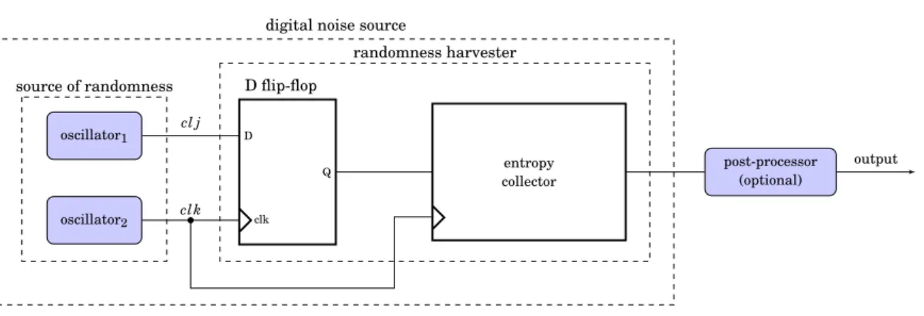
With P-TRNGs, randomness comes from a physical microscopic random process such as radioac-tive decay [59], metastability [60], biological data [61] or electronic noises like noise from Zener diodes [13] or Johnson noise [62,63,64]. The use of these sources of randomness yields various designs of P-TRNG. In this thesis, we will exclusively deal with generators implemented in logic devices like Application Specific Integrated Circuits (ASICs) and Field Programmable Gate Ar-rays (FPGAs). For these generators, the source of randomness consists of electronic noises which often manifest themselves as frequency instabilities of electronic oscillators such as Ring Oscil-lators (ROs) [65], Transient Effect Ring Oscillators (TEROs) [66], Self-Timed Ring Oscillators (STRs) [67] or Voltage-Controlled Oscillators (VCOs) [68]. They are often referred to as oscillator-based TRNGs [69], and their general structure is depicted in Figure1.2.
oscillator1 oscillator2 D clk Q D flip-flop entropy collector post-processor (optional) cl j clk output source of randomness randomness harvester digital noise source
Figure 1.2: Oscillator-based TRNG. 1.1.2.2 Randomness harvester
Because the source of randomness is a physical process, it produces a random analog signal. This signal cannot be used directly to produce random bits in logic devices. One therefore needs to convert it in a digital signal, procedure which is called digitization [24]. In logic devices, the digitization is closely related to the randomness extraction procedure. The most widespread ran-domness extraction method consists in sampling the random phenomenon at discrete times. This is done using a D flip-flop which produces a 1-bit sample of the random signal at each clock cycle [68, Section 3].
In order to assess the randomness, it is necessary to have a way of quantifying it. A common measure of randomness is the "entropy" which will be dealt with in more details in Section1.3. To ensure enough entropy at the output, it is common to allow the random process to evolve over a long period of time. This results in an entropy accumulation which yields optimal security [70]. In hardware, this is usually done with an entropy collector such as a decimator which produces one random bit out of a given number of samples [71]. In the remainder of this thesis, we will consider the association of the D flip-flop and the entropy collector as the digitizer. This choice is justified by the fact that it is part of the TRNG design and that the entropy collector is not optional like the post-processor. Even though this process uses an analog signal to produce a digital one, the term harvesting mechanism seems more appropriate than digitization since it describes the process through which randomness is extracted from the real world phenomenon.
1.1.2.3 Post-processor
The main philosophy of a TRNG is to produce sequences that cannot be recognized from those generated by an ideal RNG, i.e. they must be unbiased and uniformly distributed. However, due to imperfections that can occur both in the physical process and the harvester, the generated
se-quence may be biased. Hence it may contain a specific bit value which appears more often than the other one [72]. This is actually a serious security issue since an adversary who knows that bias can take advantage of it and guess the next values of a sequence with probability higher than 0.5 [24, Section 5.1]. To avoid such situations, the raw digital signal must go through a post-processing step before the output [10].
The goal of this post-processing step is to eliminate (or at least, reduce as much as possible) im-perfections in the raw digital signal. To achieve this goal, the post-processor usually compresses the input bit stream. The output has therefore a smaller length with better statistical qualities [73]. It is important to understand that the post-processor does not add any entropy to the bit stream, it just makes it look more random. This only increases the robustness of the generator while reducing its output bit rate. There exist various techniques for designing a post-processor, ranging from ad hoc methods to more elaborate ones such as cryptographic hash functions or re-silient functions [74,75,73].
Although there is no proper definition of which part of a TRNG should be considered as post-processor, one commonly considers the post-processor as a complex process designed to reduce imperfections present in the raw digital signal. Post-processing algorithms usually take a lot of resources and are therefore not suitable for direct implementation in hardware. Note that the use of a post-processor is not mandatory, indeed when the raw digital signal already exhibits good statistical qualities, the use of a post-processor is not relevant.
From all that precedes, one understands that the main part of interest in a TRNG is its source of randomness. Any randomness that will be used to generate random bits comes from there. It is thus of vital importance to focus on this part and understand various phenomena occurring in it.
1.2 Sources of randomness in logic devices
In Section1.1.2, we explained that the source of randomness is the most crucial part of any TRNG. Cautions must then be taken in selecting that source. In general, the design of a good TRNG is very challenging. The identification and correct exploitation of the source of randomness is by far the most challenging task in the design of a TRNG. Those implemented in logic devices are no exception to that, even though their implementation is simpler than other types of TRNGs [76,
69]. Since the security of these constructions relies on the secrecy of the key, it is important that keys are generated within the system to avoid any transport across an uncontrolled area. This explains why we focus on TRNGs that can be implemented in logic devices. Indeed, such TRNGs
constitute a source of random numbers directly available to the cryptographic constructions for various use [10]. In this section we discuss various sources of randomness present in logic devices.
1.2.1 Commonly used sources of randomness
Diverse electronic phenomena occur in logic devices. Some of them exhibit random behavior which might be used to generate random numbers. Among the most encountered electronic random phenomena, the ones listed below are commonly used.
• Metastability which is the ability of a digital electronic system to persist in an unstable equilibrium for an indefinite time [77]. This phenomenon is rare and therefore very diffi-cult to sample. It is consequently diffidiffi-cult to be sure that the output bit really depends on metastability.
• Oscillatory metastability which is the ability of a bi-stable electronic device (for example, an RS flip-flop) to oscillate between its two unstable equilibrium states, for an indefinite period [78]. It can be considered as a special case of metastability. They therefore have the same limitations. In addition, this is a phenomenon typical of a small class of bistable circuits, which raises the problem of its use on electronic circuits in general.
• Start-up value of flip-flops (or a memory element) to a random state either after power-up or periodically [79]. This is due to the fact that the behavior of the device is not always defined before the occurrence of a valid clock signal. However, there are different ways to prevent it. One of them being to initialize the flip-flop, which can be done by an adversary, and thus compromise the generation of random numbers.
• Clock jitter which is a short-term variation of an event from its ideal position [69]. This phenomenon is usually unwanted because it negatively affects most communication and high-speed systems [80]. It is however inevitable and uncontrollable, making it a prime candidate to be used as source of randomness [81, Section 1.1.1]. This is the reason why the clock jitter is a widespread source of randomness used for TRNGs implemented in logic devices [82, 71, 64, 83, 65, 84, 69, 85]. We will therefore focus on the clock jitter in the remainder of this thesis.
1.2.2 Clock jitter as a source of randomness
In logic devices, actions of digital circuits are coordinated by a special signal called the clock sig-nal [86]. In an ideal model, this signal is a square wave oscillating between two states (high and low) with a duty cycle of 50% and a stable period. However, various electronic noises affect logic devices, causing the clock period (period of the clock signal) to fluctuate around its ideal value.
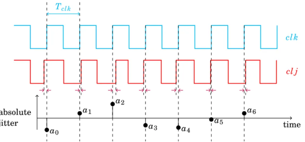
This fluctuation of the period, called clock jitter, causes edges of real-world clock signals to occur slightly earlier or later than expected as shown in Figure1.3[87, Chapter 8].
clk cl j Tclk a0 a1 a2 a3 a4 a5 a6 time absolute jitter
Figure 1.3: Illustration of clock jitter (clk: reference clock signal, cl j: jittered clock signal, ak: values of the jitter).
Based on the jitter measurement method used, various definitions of the clock jitter can be met in the literature. Most of these definitions are not standardized and therefore used with different meanings, depending on the application and the author’s background. This variety of terms used to express the concept of jitter leads to a lot of misunderstanding and confusion in the study of clock jitter. Da Dalt and Sheikholeslami showed that each of these different definitions actually falls into one of the four fundamental definitions of jitter [81, Chapter 2].
Generally speaking, jitter is the deviation of the instant at which a given event occurs, relative to a reference time frame. In the context of this thesis, as it is generally the case in the field of hardware based TRNG, the event we consider is the occurrence of (rising and falling) edges of the sampled clock signal. Note that the choice of the reference time frame is arbitrary, and is usually made in two ways: either the edges of the clock under investigation are compared to the edges of another clock, or they are compared to some previous edges of the same clock. The first approach leads to the definition of absolute and relative jitter, while the second leads to the definition of period jitter. The period jitter can be extended into a fourth jitter definition, namely the N-period jitter. These four jitter definitions are actually related to each other and will be discussed next [14].
1.2.2.1 Absolute jitter
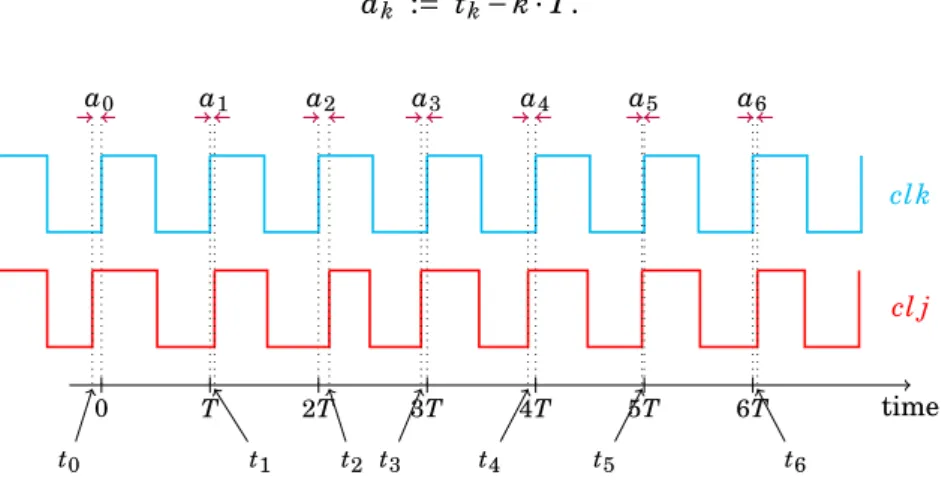
Let us consider an ideal clock signal clk, with a clock period T. If we assume that the first rising edge occurs at time t = 0, then the subsequent rising edges occur at exactly t = kT, where k ∈ N.
In the case of a non-ideal clock cl j, with nominal period3 T, the rising edges occur at times t
k
which deviate from their ideal values kT. The absolute jitter of cl j (at the k-th period) is thus defined as the time displacement of the k-th rising edge of cl j with respect to the corresponding edge of the ideal clock clk (see Figure1.4). Mathematically speaking, it is expressed as:
ak := tk− k · T. (1.9) clk cl j 0 T 2T 3T 4T 5T 6T t0 a0 t1 a1 t2 a2 t3 a3 t4 a4 t5 a5 t6 a6 time
Figure 1.4: Absolute jitter as a time deviation.
In Figure1.3, the absolute jitter is a discrete-time random signal. Mathematics of random signals will be used in Chapter2to study and characterize the jitter.Because the signal cl j and its ideal version clk both have the same period, (ak) is a zero-mean process. In some cases, when clk and
cl j are phase shifted, the positions of clk and cl j can display an offset tossuch that (ak) has mean
value tos. In that case, the absolute jitter is defined as:
ak := tk− k · T − tos, (1.10)
in a way that (ak) is still a zero-mean process. For this reason, we will consider the absolute jitter
to be a zero-mean random process.
Note that various definition exist for the absolute jitter. Indeed, it corresponds to the time error (TE) defined by the telecommunication standardization sector of the International Telecommuni-cation Union [88, Section 4.5.13].
1.2.2.2 Relative jitter
There-above, the edges of a clock signal were compared to those of its ideal version. However, no ideal clock signal exists in the real world. Thus, instead of proceeding as shown above, one can think of comparing edges of a clock signal s1 to those of another (non-ideal) one s0 having the
same nominal period T. The situation is actually the same as depicted in Figures1.3 and 1.4.
The only difference is that cl j is replaced by s1and clk by s0, both s0and s1being non-ideal clock
signals.
This setting leads to the definition of the relative jitter as a discrete-time random process rk,
where the element rk is the time displacement of the k-th rising edge tsk1 of s1 with respect to the
corresponding edge ts0
k of s0. Mathematically, it is thus expressed as:
rk := tsk1− tsk0. (1.11)
Since both s0 and s1 have respective absolute jitter processes ¡ask0¢ and ¡ask1¢, it is possible to
express the relative jitter in term of absolute jitters of s0 and s1. By the use of Equation (1.9), we
can rewrite Equation (1.11) as:
rk = ask1− ask0. (1.12)
Note that for the same considerations as for the absolute jitter, the relative jitter is a zero-mean random process.
1.2.2.3 Period jitter
The two jitter definitions provided above are based on comparing the edges of the clock signal to the edges of another clock signal. However, it is also possible to compare the position of an edge to the position of the previous edge of the same clock signal. Assume that, for a clock signal, a specific rising edge occurs at time tk and the next one at time tk+1, then tk+1− tk represents one
realization of the clock period. Comparing this realization of the clock period to its nominal value leads to the definition of the period jitter.
The period jitter is defined as a discrete-time random process (pk), for which each pk is the time
deviation of the k-th clock period from its nominal value. Figure1.5illustrates this concept and shows that the k-th clock period is actually the time difference of the (k + 1)-th and k-th rising edges. The k-th sample of the period jitter can then be mathematically expressed as:
pk := (tk+1− tk) − T, (1.13)
where T is the nominal period of the clock signal. If we call Tk := tk+1− tk, the current clock
period, Equation (1.13) becomes:
pk = Tk− T. (1.14)
Note that period jitter can also be expressed in term of absolute jitter. Indeed, using Equa-tion (1.9), Equation (1.13) becomes:
T T T
T0 p0 T1 p1 T2 p2
time Figure 1.5: Illustration of the period jitter.
The period jitter is sometimes (wrongly) named cycle-to-cycle jitter [89, 90]. Indeed, from the JEDEC standard JESD65B [91, Page 10], cycle-to-cycle jitter is the variation in cycle time of a signal between adjacent cycles, over a random sample of adjacent cycle pair. It is thus the difference between two consecutive clock periods and it indicates how much one period of the clock differs from the previous one. If we denote by (cck) the random process of cycle-to-cycle
jitter, one has:
cck := Tk+1− Tk, (1.16)
which can be expressed in terms of period jitter as:
cck := pk+1− pk. (1.17)
This latter equation shows that these two notions are not the same, even though they are related. 1.2.2.4 N-Period jitter
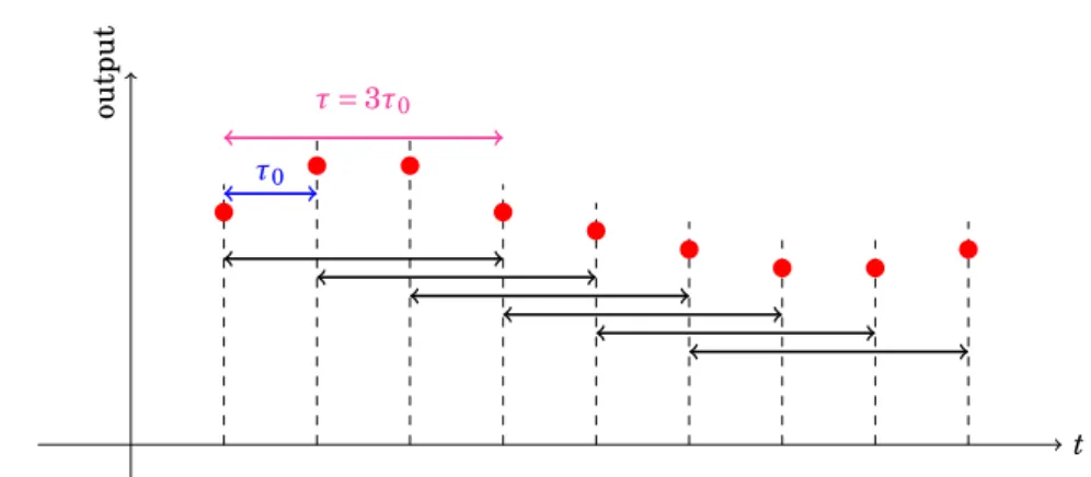
Because the designer of a circuit aims at reducing the clock jitter, it appears that clock jitter is very small compared to the clock period (approximately 1‰ of the clock period). In order to guar-antee enough entropy, it is common practice to compare the time deviation of a clock edge not to the immediate preceding one, but to the N-th previous one, as illustrated in Figure1.6.
This procedure leads to the definition of N-period jitter as the discrete-time random process (pk(N)), where each element pk(N) is the deviation around the nominal value of the position
of one clock edge with respect to the N-th previous edge. Mathematically, pk(N) is expressed as
the deviation of the time difference between the k-th and the (k + N)-th edges from the nominal value NT, that is:
5T
Tk Tk+1 Tk+2 Tk+3 Tk+4
pk(5)
time
tk tk+1
Figure 1.6: Illustration of the N-period jitter.
From this definition, one can observe that Equation (1.13) is a special case of Equation (1.18) for N = 1. It thus appears that N-period jitter is a generalization of the period jitter discussed above. Moreover, considering that tk+N− tk is the duration of the N periods of the clock following the
k-edge, the N-period jitter can be written as: pk(N) = Ãk+N−1 X i=k Ti ! − NT, (1.19)
where Tiindicates the i-th clock period. From Equation (1.19), one can derive:
pk(N) = k+N−1 X i=k (Ti− T) = k+N−1 X i=k pi, (1.20)
where each pi represents the period jitter of the i-th clock period. It then follows that the
N-period jitter is the sum of the N-period jitter over N consecutive N-periods. Because it originates from the accumulation of the jitter over consecutive periods, various authors refer the N-period jitter as the accumulated jitter [92,84,93,69,66,60,94]. As in the case of period jitter, it is possible to express the N-period jitter in terms of the absolute jitter:
pk(N) = ak+N− ak. (1.21)
Equation (1.21) shows that the N-period jitter is what the International Telecommunication Union refers to as the time interval error [88, Section 4.5.14].
The various above-mentioned types of jitter are all mutually related. This shows that from a physical point of view, these various definitions refer to the same phenomenon affecting the clock signal. Their specificities come from the method used to measure this phenomenon.
In real-world, signals are all jittered, so it is the relative jitter we often have access to. However, when two signals are independent from each other, it is possible to transfer the jitter of one of these signals to the other. This results in an ideal signal, and a jittered one containing the
contribution of the jitters of both signals, allowing the absolute jitter to be evaluated [95]. Since this approach simplifies computations, we will focus on the absolute jitter, which will be simply denoted jitter in the remainder of this thesis.
1.2.3 Jitter sources
In section 1.2.2, we briefly explained what the clock jitter is and its different representations. In order to have a better understanding of this phenomenon, it is common to break it down and identify its different parts. Since each component of the jitter has its own characteristic and phys-ical meaning, the separation of the jitter can be used to investigate its cause. The separation of the jitter is usually made based the nature of the jitter component as depicted in Figure1.7[81, Section 2.2.6]. Total Jitter Random Jitter Deterministic Jitter Duty Cycle Distortion Data Dependent Jitter Bounded Uncorrelated Jitter Power supply noise Cross-talk / external noise Applied sinusoidal
Figure 1.7: Overview of the jitter components.
In Figure1.7, we see that jitter has two main components: a random component and a determin-istic component. There are several methods to determine if the jitter is of random or determindetermin-istic origin [96, Section 8]. The simplest one is the observation of the histogram. A histogram in the shape of a Gaussian is often indicative of a random jitter.
Random jitter includes all components for which the probability density is not bounded [96, Sec-tion 7.2.2]. This means that the range of the random jitter is not limited. In electronic circuits, it is produced by electronic noises such as thermal noise, flicker noise and shot noise [96, Section 9.2.2.1]. It is generally described as a random phenomenon with a zero mean Gaussian distribu-tion, and therefore characterized by its variance or standard deviation.
The deterministic jitter consists of the components of the jitter for which the probability density is bounded [96, Section 7.2.3]. The most common causes of deterministic jitter are instabilities
from the power supply, cross-talk from other signals or channels, distortion of the duty cycle, limitation of the channel bandwidth. Depending on the origin mechanism, it is possible to divide the deterministic jitter into several sub-categories, the most common being listed below.
• Duty cycle distortion: due to asymmetries in the duty cycle when both rising and falling edges of a clock signal are used in a given application.
• Data dependent jitter: specific to the data pattern transmitted in the same path as the signal under test.
• Bounded-uncorrelated jitter: present in the serial digital data, but bears no correlation with the transmitted data. It has three main sources: (1) power supply noise that affects the launched signal, (2) cross-talk that occurs during transmission and (3) sinusoidal applied to the receiver input for jitter tolerance measurements.
To ensure that generated numbers are random, it is necessary that the only jitter components used are random. In other words, it is imperative to mitigate the influences of deterministic com-ponents of the jitter. However, some random comcom-ponents present security risks, and therefore need to be eliminated as well. In order to respond more effectively to security issues related to the generation of random numbers, it is possible to consider another subdivision of jitter, taking into account not only its nature, but also its source (local or global) as shown in Figure1.8.
Clock jitter sources
Local sources
Random sources (e.g thermal noise, flicker noise)
Deterministic sources (e.g cross-talk)
Global sources
Random sources
(e.g random noise from EMI, power supply) Deterministic sources
(e.g deterministic noise from EMI, power supply)
Figure 1.8: Overview of the jitter sources.
Global sources (random and deterministic) are external sources, and therefore potentially ma-nipulable. An adversary can therefore a priori exploit these sources in order to deteriorate the quality of the randomness, and thus reduce the security of cryptographic systems. Thus, in addi-tion to reducing the effects of deterministic sources, it is important to reduce the effects of global sources on the generation of random numbers. For this purpose, it is possible to use two identical
oscillators in Figure 1.2. Indeed, because they are subjected to the same phenomena, they will display the same effects due to these global sources. Thus, as a differential principle, these effects will cancel each other during sampling [97].
Random local sources are internal and thus non-manipulable. They are therefore the only rec-ommended ones for generating random numbers for cryptography. Consequently, it is mandatory that the jitter measurement methods evaluate only random local components. This problem is not simple and will be discussed in more detail in Chapter2.
1.3 Entropy
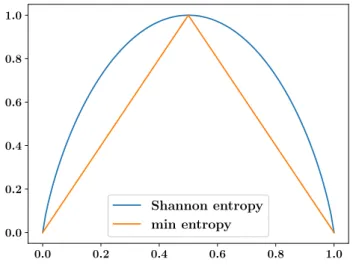
The term entropy was first introduced in 1865 by Clausius in thermodynamics [98]. It derives from the combination of an ancient English word and a Greek word, which together mean inside transformation. The entropy characterizes the level of disorganization, diversity, uncertainty or randomness of a given system [99]. It is therefore a suitable tool to evaluate the quality of a sequence of random numbers. In the field of information theory, the notion of entropy was brought by Shannon [100], then generalized by Rényi [101]. We will give a brief overview of various entropies used in information theory and which will be required for the rest of this thesis.
1.3.1 Rényi entropy
1.3.1.1 Understanding entropy
Let X be a valued random variable with imageX, in order to know how random X is, one needs to compute its entropy or level of randomness. The higher this entropy is, the more random X is. If we call PX, the probability distribution4 of X, andα∈ R+à {1}, Rényi defined the entropy of X
of orderαas: Hα(X) := 1 1 −αlog à X x∈X p(x) α ! . (1.23)
It appears from Equation (1.23) that Hα(X) depends on the probability distribution of X. Since
this probability is related to the random variable X, the entropy is commonly considered as a function of X. Note that the definition of entropy is given here using base 2 logarithm. However, it is possible to define it using any base logarithm [103]. In this thesis, we will however restrict to the base 2 logarithm. For this reason, the entropy will be expressed in bits.
4The probability distribution, P
X, of the random variable X is defined for any x∈X as [102, Section 2.1]:
PX(x)=P(X=x) =P({ω ∈Ω : X(ω)=x}). (1.22)
The entropy Hα(X) provides a measure of the quantity of unpredictable information contained
in the random variable X. This can be understood as the amount of information we obtain by observing the outcome of the experiment involving X [104]. It turns out that the more difficult it is to correctly guess the outcome of X, the more information we get by observing is actual out-come. For example, if X is deterministic, thenX contains only one value, that is X = {x} and thus p(x) = 1. One does not need to observe the outcome of X before to know that it will be x. He therefore gains no information by observing the outcome of X. One may note that in this case Hα(X) = 0, which is actually a result characterizing any deterministic phenomenon.
From what precedes, one understands that the underlying phenomenon responsible of the TRNG operation must have as high entropy as possible to ensure a high difficulty in guessing the output of the considered TRNG.
1.3.1.2 General properties of Rényi entropy
Equation (1.23) shows that Rényi entropy is actually a parametric family of entropy measures forα∈ R+à {1}. The goal of Rényi when defining his entropy was to have the most general class
of information measures that preserve the additivity of statistically independent systems and are compatible with probability axioms [101]. The limit classes, whenαapproaches 1 and when αapproaches infinity, lead to two entropy measures interesting for the field of random number
generation.
Continuous extension of Rényi entropy atα= 1 From Equation (1.23), Rényi entropy is not
defined forα= 1. However, for a given X, the functionα7−→ Hα(X) has a limit asαapproaches 1.
The proof reveals that:
lim
α→1Hα(X) = − Xx∈X p(x)log p(x). (1.24)
This limit is the Shannon entropy which will be detailed in Section1.3.2. From the continuous extension theorem, one can then consider Rényi entropy defined forα∈ R+.
Min entropy For a given random variable X, if X is such that max
x∈X p(x) exists, then one can
prove: lim α→∞Hα(X) = −log µ max x∈X p(x) ¶ . (1.25)
This limit is called min entropy and denoted H∞(X). Knowing that log is a continuous and
non-decreasing function, one can write: logµmax
x∈X p(x)
= max