HAL Id: tel-01484031
https://tel.archives-ouvertes.fr/tel-01484031
Submitted on 6 Mar 2017
HAL is a multi-disciplinary open access archive for the deposit and dissemination of sci-entific research documents, whether they are pub-lished or not. The documents may come from teaching and research institutions in France or abroad, or from public or private research centers.
L’archive ouverte pluridisciplinaire HAL, est destinée au dépôt et à la diffusion de documents scientifiques de niveau recherche, publiés ou non, émanant des établissements d’enseignement et de recherche français ou étrangers, des laboratoires publics ou privés.
Application on Beirut
Christelle Salameh
To cite this version:
Christelle Salameh. Ambient vibrations, spectral content and seismic damages : new approach adapted to the urban scale. Application on Beirut. Risques. Université Grenoble Alpes, 2016. English. �NNT : 2016GREAU008�. �tel-01484031�
THÈSE
Pour obtenir le grade de
DOCTEUR DE LA COMMUNAUTÉ UNIVERSITÉ
GRENOBLE ALPES
Spécialité : Sciences de la Terre, l’Univers et l’Environnement Arrêté ministériel : 7 août 2006
Présentée par
Christelle SALAMEH
Thèse dirigée par Pierre-Yves BARD et
codirigée par Bertrand GUILLIER et Jacques HARB
préparée au sein de l’Institut des Sciences de la Terre dans l'École Doctorale Terre, Univers, Environnement
Vibrations ambiantes, contenu
spectral et dommages sismiques:
nouvelle approche adaptée à
l’échelle urbaine. Application à
Beyrouth.
Thèse soutenue publiquement le « 21 Juin 2016 », devant le jury composé de :
M., Michel, KHOURI
Pr. Ass., Université Libanaise, Beyrouth, Rapporteur
M., Jean-François, SEMBLAT
DR, IFSTTAR, Paris, Rapporteur
M., Michel, BOUCHON
DR, CNRS, Grenoble, Président du jury
M., Donat, FÄH
Pr., ETH, Zürich, Examinateur
M., Fernando, LOPEZ-CABALLERO
Pr. Ass., Ecole Centrale, Paris, Examinateur
M., Jacques, HARB
Pr, Université Notre Dame, Beyrouth, Co-directeur de thèse
M., Bertrand, GUILLIER
CR, ISTerre, Université Grenoble Alpes, Co-directeur de thèse
M., Pierre-Yves, BARD
IGPC, ISTerre, Université Grenoble Alpes, Directeur de thèse
M., Stéphane, GRANGE
This thesis is dedicated to my mom Diana, my dad Marcel and my
brother Dany and to the loving memory of my uncle Roukoz Bechara.
Thank you for everything.
Il a été observé maintes fois dans les enquêtes post-sismiques que les structures ayant des fréquences similaires à celles du sol de fondation présentent des dommages beaucoup plus importants (Caracas 1967, Mexique 1985, Pujili, Equateur 1996; L'Aquila 2009). Cette observation de bon sens n'est cependant que très peu, ou de façon très indirecte, prise en compte d'une part dans les réglementations parasismiques (échelle du bâtiment), et d'autre part dans les études de risque et de scénario à l'échelle urbaine. On assiste ainsi souvent à un niveau de précision incohérent entre les études d'aléa, qui sont maintenant à même de cartographier de manière fiable les fréquences de sol, les possibilités actuelles en matière d'analyse du comportement dynamique des bâtiments, et les cartes de vulnérabilité et de risque finales. Une analyse numérique complète pour étudier l'effet de coïncidence entre les fréquences du sol et du bâtiment est effectuée. Un ensemble de 887 profils de sol réalistes est couplé avec un total de 141 oscillateurs élastoplastiques à un degré de liberté, et leurs réponses combinées (non linéaires) sont calculées à la fois pour un comportement de sol linéaire et non-linéaire, pour un grand nombre (60) de signaux d'entrée avec différents niveaux de PGA et contenu fréquentiel. Les dommages associés sont quantifiés sur la base du déplacement maximal comparé à la fois par rapport aux déplacements élastiques et ultimes, selon les recommandations du projet européen RISK-UE (Lagomarsino et Giovinazzi, 2006), et par rapports aux dommages obtenus dans le cas d’un bâtiment similaire situé sur le substratum rocheux. La corrélation entre les incréments de dommages entre sol et rocher et un certain nombre de paramètres simples mécaniques et de chargement est ensuite analysée en utilisant une approche de réseau neuronal. Les résultats soulignent le rôle clé joué par le rapport de fréquence bâtiment/sol, même lorsque le sol et le bâtiment se comportent de manière non linéaire; d'autres paramètres importants sont le niveau de PGA, le contraste d’impédance sol/rocher et la ductilité du bâtiment. Une enquête numérique spécifique basée sur la simulation du bruit ambiant pour l'ensemble des 887 profils indique également que l'impact du contraste d’impédance sol/rocher peut être cohéremment remplacé en utilisant l'amplitude du rapport H/V. Aussi l'effet de coïncidence apparaît comme une observation importante, non seulement dans la réponse de l'analyse des sites linéaires, mais aussi dans la réponse d'un site non-linéaire: en dépit d'un niveau important de non-linéarité atteint la coïncidence spectrale se produit, mais à un rapport de fréquence décalé vers des valeurs inférieures. La méthode élaborée permet une mise en œuvre très facile, en utilisant des mesures de vibrations ambiantes, tant au niveau du sol et à l'intérieur des bâtiments. Un exemple d'application très illustratif est représenté pour la ville de Beyrouth (Liban).
It has been observed repeatedly in post-seismic investigations that structures having
frequencies close to foundation soil frequencies exhibit significantly heavier damages
(Caracas 1967, Mexico 1985, Pujili, Ecuador 1996; L’Aquila 2009). However, these
observations are generally not taken directly into account neither in present-day seismic
regulations (small scale), nor at large-scale seismic risk analysis. We thus encounter
frequently an incoherent precision level between hazard studies that are capable of reliably
mapping the ground frequency, the actual possibilities of analyzing the dynamic behavior of
the building, and the final vulnerability and risk maps. A comprehensive numerical analysis to
investigate the effect of coincidence between soil and building frequencies is performed. A
total of 887 realistic soil profiles are coupled with a set of 141 elastoplastic oscillators with a
single degree of freedom and their combined (non-linear) response are computed both for
linear and non-linear soil behavior, for a large number (60) of input signals of various PGA
levels and frequency contents. The associated damage is quantified on the basis of the
maximum displacement as compared to both yield and ultimate post-elastic displacements,
according to the RISK-UE European project recommendations (Lagomarsino and Giovinazzi,
2006), and compared with the damage obtained in the case of a similar building located on
bedrock. The correlation between this soil/rock damage increment and a number of simplified
mechanical and loading parameters is then analyzed using a neural network approach. The
results emphasize the key role played by the building/soil frequency ratio even when both soil
and building behave non-linearly; other important parameters are the PGA level, the soil/rock
impedance contrast and the building ductility. A specific numerical investigation based on
simulation of ambient noise for the whole set of 887 profiles also indicates that the impact of
soil/rock impedance contrast may be satisfactory replaced using the amplitude of H/V ratio.
Moreover the effect of coincidence appears to be an important observation not only in the
linear site analysis response but also in the nonlinear site response: in spite of a large
nonlinearity level reached spectral coincidence occurs, however at a shifted frequency ratio
towards lower values. The elaborated method allows a very easy implementation, using
ambient vibration measurements both at ground level and within buildings. A very illustrative
example application is shown for the city of Beirut (Lebanon).
First I would like to thank my supervisors Pierre-Yves Bard, Bertrand Guillier and Jacques Harb for their supervision and positive energy. Working with you was more than great both on scientific and especially on human side. Thank you for guiding me and keeping me motivated until the last moment which was the hardest.
Thanks to Cécile Cornou, Armand Mariscal and Christophe Voisin for their constant help and guidance throughout the years and the many memories we had especially when doing the field measurements.
Jean-Francois Semblat, Michel Bouchon, Donat Fah, Fernando-Lopez Caballero, Stéphane Grange, Michel Khouri thank you so much for accepting to be in my thesis committee and coming all along from different parts of the world to participate into my defense. The fruitful discussions we had and the invaluable feedbacks about my manuscript and presentation were priceless for the improvement of my work. Your presence encouraged me to give my best and enlarged many horizons to continue in the research field. I really appreciate it. I would like to thank also Fabien Bonilla for his time and help especially in the nonlinear part.
A special thanks goes also to the Libris research program (ANR RiskNat 2009-006) in collaboration between the laboratories ISTerre (Grenoble, France), Lebanese Geophysical Research Center (CRG), Saint-Joseph University of Beirut, Notre Dame University-Louaizé NDU, IPGP, EDYTEM, CETE, and IRD (Institut de Recherche pour le Développement) who supported and funded this work. I would like to thank the municipalities of Jdeideh and Bourj Hammoud for their help in the access to the buildings, Jocelyne Gérard, Rita Zaarour and Nada Saliba for making use of the building inventory database and the Labex OSUG@2020 for financial support.
Big thanks to all ISTerre group (colleagues, researchers, friends). I am so lucky that I worked in this lab. I combined research, fun, friendship in one place. That was awesome; I will miss it so much.
Thank you to all my friends Lebanese and international who were always there for good times and bad times, for their support and motivation, during this journey. Special Thanks to Perla, Pamela, Cherine, Elionore, Elias, Rosy, Nancy, Rita, Micha, Jimmy, Mohamad, Raja, Elie, Capucine, Kaveh, Zabedine, Boumédiène, Joe and all the “Hangout” (my second family in France).
A special thanks for the persons that work in the shadow, i.e. the ISTerre informatics staff (Kamil, Jean-Noël, Hafid and Rodolphe) and the administrative group (thank you Cécile Cretin, Jacques Pellet, Karine de Palo) without which my work would have been much more complicated.
And finally the warmest thanks go to my family for their unconditional support, without you I wouldn’t be here. Mom, Dad, Dany thank you for trusting in me and helping me despite the many miles that separate us.
Chapter 1: General Introduction ... 16
1.1. Motivation of the thesis ... 17
1.2. Outline of the thesis ... 21
Chapter 2: Consideration of spectral coincidence in seismic vulnerability and risk assessment using Artificial Neural Network (ANN) approach ... 24
2.1. Introduction ... 25
2.2. Seismic risk and vulnerability assessment ... 27
2.2.1. The seismic hazard estimation ... 27
2.2.2. Vulnerability and damage estimation methods ... 28
2.3. Intermediate approach: Oscillator with single-degree-of-freedom over a horizontal layer ... 39
2.3.1. Elastoplastic SDOF oscillator ... 39
2.3.2. Seismic waves propagation through the soil: reflectivity method ... 40
2.3.3. Response of the damped oscillator ... 41
2.3.4. Theoretical model: Soil and structure combined ... 42
2.3.5. Traditional statistical analysis for one horizontal layer over half-space ... 43
2.4. Realistic Case: Oscillator with single-degree-of-freedom on a multi-layered profile ... 49
2.4.1. Structure database ... 49
2.4.2. Soil profile database ... 50
2.4.3. Definition of Damage increment index (DI) ... 58
2.4.4. Traditional statistical analysis ... 60
2.5. Artificial Neural Network (ANN) approach ... 64
2.5.1. What is the ANN approach? ... 64
2.5.2. Application of ANN approach in the present study ... 74
2.6. Conclusion ... 94
Chapter 3: Testing a convenient proxy for site amplification: H/V amplitude ... 96
3.1. Introduction ... 97
3.2. Ambient noise vibration ... 98
3.2.1. More than a century of research ... 98
3.2.2. Ambient noise origin ... 101
3.3. Numerical simulation of ambient noise in a horizontally stratified, 1D medium ... 102
3.3.1. Green Functions Computation- Hisada wave-number approach ... 103
3.3.2. Soil Models-Propagation medium ... 104
3.3.3. Sources and receivers configuration ... 105
3.3.4. Horizontal-to-Vertical (H/V) spectral ratio computation ... 107
3.3.5. Advantages and limitation of H/V method ... 110
3.4. Description of the data set ... 110
3.4.1. Statistical analysis of the f0HV, A0HV derived from noise synthetics ... 110
3.4.2. Comparison between synthetic and theoretical frequencies and amplitudes ... 112
3.5. H/V amplitude: a tool in the seismic vulnerability and risk assessment ... 113
3.5.1. The Neural Network Structure: A0HV, Vs30,Vs10 Vbedrock/Vs30 and Vbedrock/Vs10 ... 114
3.5.2. A0HV, Vs30,Vs10, Vbedrock/Vs30 and Vbedrock/Vs10: what is the best proxy? ... 117
3.6. Conclusions ... 127
4.2. Nonlinear computation methods ... 132
4.2.1. Visco-elastic equivalent linear approach ... 132
4.2.2. Nonlinear model ... 135
4.3. Database description ... 138
4.3.1. Soil model ... 138
4.3.2. Non-linearity parameters ... 140
4.4. Results on non-linear site response: a statistical outline ... 142
4.4.1. Non-linear indicator: Shear Strain ... 143
4.4.2. Effect of soil parameters on nonlinearity ... 143
4.4.3. Depth of maximum strain ... 147
4.4.4. PGV/Vs as a strain proxy ... 148
4.4.5. Example results for eight, highly non-linear, soil profiles ... 150
4.4.6. Evolution of transfer function with the degree of non-linearity... 154
4.4.7. Effect of nonlinearity on surface PGA ... 156
4.5. Impact of soil non-linearity on damage increment ... 157
4.5.1. Effect of nonlinearity on the maximum displacement at the top of the structure ... 158
4.5.2. Effects of the frequency on the displacement ... 160
4.5.3. Neural Network Architecture ... 160
4.5.4. Results of Neural network approach and effect of soil nonlinearity on the structure’s behavior ... 162
4.6. Conclusion ... 165
Chapter 5: Seismic response of Beirut (Lebanon) buildings: Instrumental results from ambient vibrations ... 167
5.1. Introduction ... 168
5.2. Period estimation in seismic design codes ... 169
5.3. Experimental estimation of dynamic parameters using ambient vibration method ... 171
5.4. Beirut: Seismic risk, geology and recent construction history ... 172
5.4.1. Seismic Hazard assessment of Beirut ... 172
5.4.2. Beirut geology ... 174
5.4.3. Construction history of Beirut ... 175
5.5. Extraction of fundamental period and damping of buildings ... 180
5.5.1. Site investigation of the building ... 182
5.5.2. Fundamental period of buildings ... 183
5.5.3. Measurement of building damping ... 185
5.6. Empirical relationships specific to Beirut using ambient vibration ... 185
5.6.1. Comparison with building codes and other empirical relationships ... 185
5.6.2. Empirical relationships for Beirut buildings accounting for the soil stiffness ... 188
5.7. Discussion ... 191
5.8. Elaboration of Beirut city-wide vulnerability maps ... 192
5.8.1. Database description ... 192
5.8.2. Application of the ANN model on the city of Beirut ... 195
5.8.3. Maps processing ... 200
5.9. Comparison with the Lebanese Seismic Code ... 207
5.10. Conclusion ... 209
Acknowledgments ... 211
References ... 219
Appendix A Tables for Hazus and Risk-UE methods ... 240
Appendix B Soil Profiles Database ... 247
Appendix C Matrices of weights and biases ... 259
Appendix D NOAH Code ... 279
Appendix E Beirut ... 285
List of Figures
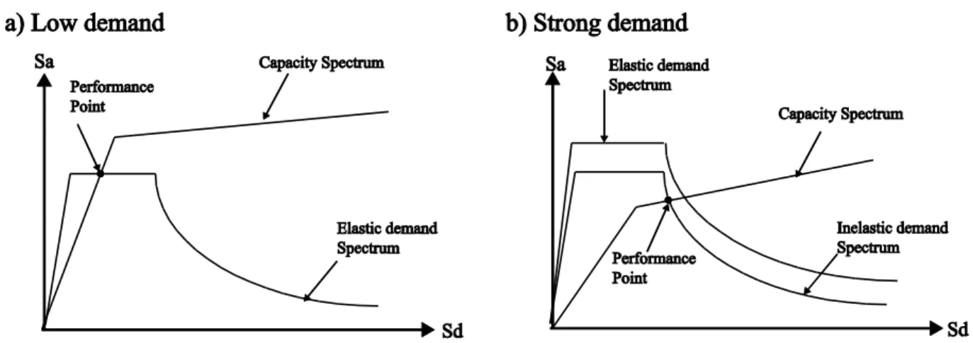
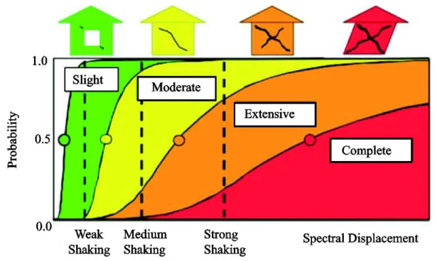
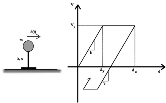
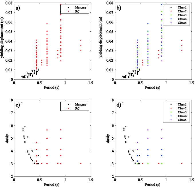
Fig. 1.1: Individual earthquakes from 800 to 2011 with more than 50,000 fatalities from USGS catalog (Holzer and Savage 2013). ... 17 Fig. 1.2: Map of global seismic hazard and world population; the red circle corrresponds to Beirut city (Lebanon) (Karklis 2010). ... 18 Fig. 1.3: Representation of the damages caused to buildings with respect to their height following the 1985 earthquake in Mexico City. ... 19 Fig. 2.1: Concept of a double resonator: structure defined by its stiffness K and mass M based on a horizontal layer defined by thickness, density, Vs and quality factor; the total transfer function TF of soil and structure shows amplification of the amplitude of vibration at the soil/structure frequencies coincidence. ... 27 Fig. 2.2: Vulnerability classes; classification using EMS 98 method (Grunthal 1998). ... 32 Fig. 2.3: Macroseismic method: a) vulnerability curves for different masonry building typologies; expected damage μD = 1.7 for M4 typology when I = 8.5, b) fragility curves for the building typology M4 as a function of I; damage distribution for I = 8.5 (Lagomarsino and Giovinazzi 2006). ... 33 Fig. 2.4: Representation of the fundamental mode and the amplitude of the mode shape at level i. 34 Fig. 2.5: Capacity spectrum method: (a) development of pushover curve, (b) conversion of pushover curve to capacity diagram, (c) conversion of elastic response spectrum from standard format to A-D format, and (d) determination of displacement demand (Chopra and Goel 1999). ... 36 Fig. 2.6: Performance point identification: intersection between the seismic demand and the capacity curve at a) low demand case and b) strong demand. ... 37 Fig. 2.7: Damage thresholds identified on the capacity curve based on the Risk-UE project (Lagomarsino and Giovinazzi 2006). ... 38 Fig. 2.8: Fragility curves for different levels of damage: slight, moderate, extensive, complete (FEMA 2003). ... 39 Fig. 2.9: SDOF system defined by its mass m, its rigidity k, its damping c and a perfect elasto-plastic behavior. ... 40
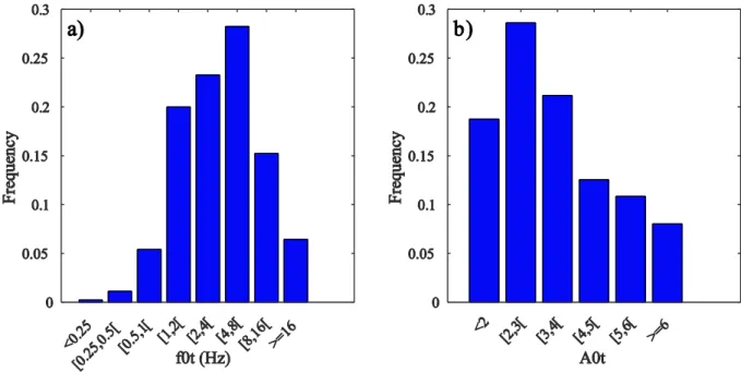
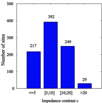
Fig. 2.10: Modification of the signal while propagating through the different layers of a stratigraphic medium. ... 41 Fig. 2.11: Distribution of signals with respect to PGA (m/s2). ... 42 Fig. 2.12: Impedance contrast effect: Variation of the top displacement (m) in function of time for c=2, c=4 and c=8 with a fixed PGA=3.35 m/s2, soil frequency (fsoil= 3Hz), structure frequency (fstruct=4 Hz) and ductility limit (dy=0.005 m). ... 44 Fig. 2.13: Freqeuncy ratio effect: Variation of the top displacement (m) in function of time for fstruct/fsoil<1, fstruct/fsoil>1and fstruct/fsoil~1with a fixed signal (PGA=1.78 m/s2), impedance contrast (c=8), and structure ductility limit (dy=0.005 m). ... 45 Fig. 2.14: PGA effect: Variation of the top displacement (m) in function of time for PGA=0.64 m/s2, PGA=1.78 m/s2, PGA=3.35 m/s2, with a fixed soil (fsoil=6 Hz, c=8), and fixed structure (fstruct=1Hz, dy=0.005 m). ... 46 Fig. 2.15: Variation of the maximum structural displacements ratio between soil and rock conditions as a function of structure/soil frequency ratio for various impedance contrasts c in the horizontal layer over half-space case; for different PGA classes for dy=0.005m. ... 48 Fig. 2.16: Distribution of the 141 structures taken from Lagomarsino and Giovinazzi (2006): yielding displacement dy (m) as function of the period (s) with respect to a) 2 main categories Masonry and RC and b) the 5 tyopology classes; du/dy in function of the period (s) with respect to c) 2 main categories Masonry and RC and d) the 5 typology classes; ... 50 Fig. 2.17: Frequency distribution of a) the fundamental frequency, b) and the amplification factor extracted from the transfer functions. ... 52 Fig. 2.18: Correlation between the fundamental frequency f0t (Hz) extracted from the 1D numerical Kennet method and the bedrock depth (m). The dashed lines represent the constant velocity Vs in m/s for the values 200, 400, 600, 800. ... 52 Fig. 2.19: Distribution of the sites with respect to the impedance contrast categories. ... 54 Fig. 2.20: Linear regression between amplification factor identified on the transfer function (A0t)
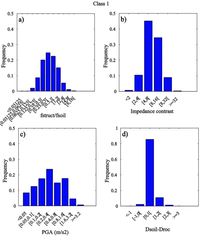
LVZ, b) depth of LVZ (m), c) the thickness of LVZ (m), and d) the local contrast. ... 56 Fig. 2.23: Frequency distribution of the average shear wave velocity over a depth of a) 10 m (Vs10), b) and 30 m (Vs30 ). ... 57 Fig. 2.24: Distribution of the sites with respect to the EC8 soil classification according to Vs30. ... 58 Fig. 2.25: Damge index definition based on the damage state and dispalcements tresholds of Lagomarsino and Giovinazzi. The black line is the capacity curve, the red line corresponds to the new defined damage index (2006). ... 60 Fig. 2.26: Number of models with destructed and not destructed structures both on soil and the corresponding bedrock obtained in each typology class. ... 60 Fig. 2.27: Damage increment between soil and rock as a function of the ratio of frequencies structure/soil for different ranges of PGA (m/s2) considering damage levels D0 to D3 in the case of the 887 real soil profiles for different impedance contrast according to typology class 5. ... 62 Fig. 2.28: Percentage of collapsed structures (D4) on soil as a function of fstructure/ fsoil, PGA (m/s2) and for different classes of buildings as defined by Lagomarsino and Giovinazzi (2006). ... 63 Fig. 2.29: Diagram of a single artificial neuron and its activation function. ... 65 Fig. 2.30: Artificial neural network ANN diagram displaying the Input, Hidden and Output layers with respectively Ii, Hi and Oi the input, hidden and output neurons. ... 65 Fig. 2.31: Simple illustration of a well‐fit model and an overfitting of a model (Goh 2004). ... 70 Fig. 2.32: An example of the evolution of the tain, validation and test performances with respect to the number of iterations and detection of an early stopping point. ... 71 Fig. 2.33: The regression plot for the three subsets : a) training, b) validation and c) test. The dotted lines represents the perfect fit between the two values (R2=1), the solid lines represents the real correlation between the computed output and the initial target. ... 73 Fig. 2.34: Percentage of the synaptic weights for the 4 inputs in the ANN. ... 75 Fig. 2.35: Distribution of the parameters according to ANNclass1: the inputs a) struct/soil frequencies, b) impedance contrast, c) PGA(m/s2), and the output d) Dsoil-Droc. ... 77 Fig. 2.36: Distribution of the parameters according to ANNclass2: the inputs a) struct/soil frequencies, b) impedance contrast, c) PGA (m/s2), and the output d) Dsoil-Droc. ... 78 Fig. 2.37: Distribution of the parameters according to ANNclass3: the inputs a) struct/soil frequencies, b) impedance contrast, c) PGA (m/s2), and the output d) Dsoil-Droc. ... 79 Fig. 2.38: Distribution of the parameters according to ANNclass4: the inputs a) struct/soil frequencies, b) impedance contrast, c) PGA (m/s2), and the output d) Dsoil-Droc. ... 80 Fig. 2.39: Distribution of the parameters according to ANNclass5: the inputs a) struct/soil frequencies, b) impedance contrast, c) PGA (m/s2), and the output d) Dsoil-Droc. ... 81 Fig. 2.40: Choice of the hidden neurons number with respect to AIC and RMSE ... 82 Fig. 2.41: Architecture of the Neural Network: Inputs are the structure soil frequencies ratio, the impedance contrast and the PGA; the output is the damage increment between soil and structure. A neural network model was analyzed for each of the 5 typology classe. ... 83 Fig. 2.42: Regression plot for Class 2: a) Training , b) Validation and c) Test set. The dotted lines represents the perfect fit between the two values (R2=1), the solid lines represents the real correlation between the computed output and the initial target. ... 85 Fig. 2.43: Distribution of errors with respect to the training, validation and test sets for the
ANNclass2. ... 86
Fig. 2.44: Percentage of synaptic weights of the 3 inputs in the neural network approach: fstruct/fsoil, impedance contrast and PGA according to the 5 typology classes (Lagomarsino and Giovinazzi 2006). ... 88 Fig. 2.45: Class 1:Variation of the increment of damage between soil and structure in function of the structure and soil frequencies ratio and: a) the impedance contrast , and b) for 4 values of c, for different ranges of PGA (m/s2); c) the PGA (m/s2), and d) for 4 values of PGA , for different ranges of c ... 89 Fig. 2.46: Class 2:Variation of the increment of damage between soil and structure in function of the structure and soil frequencies ratio and: a) the impedance contrast , and b) for 4 values of c, for different ranges of PGA (m/s2); c) the PGA (m/s2), and d) for 4 values of PGA , for different ranges
the structure and soil frequencies ratio and: a) the impedance contrast , and b) for 4 values of c, for different ranges of PGA (m/s2); c) the PGA (m/s2), and d) for 4 values of PGA , for different ranges of c. ... 91 Fig. 2.48: Class 4:Variation of the increment of damage between soil and structure in function of the structure and soil frequencies ratio and: a) the impedance contrast , and b) for 4 values of c, for different ranges of PGA (m/s2); c) the PGA (m/s2), and d) and d) for 4 values of PGA , for different ranges of c. ... 92 Fig. 2.49: Classe 5:Variation of the increment of damage between soil and structure in function of the structure and soil frequencies ratio and: a) the impedance contrast , and b) for 4 values of c, for different ranges of PGA (m/s2); c) the PGA (m/s2), and d) for 4 values of PGA , for different ranges of c. ... 93 Fig. 2.50: Perspective: Heaviside and Gaussian curves to approximate the Neural Model. ... 95 Fig. 3.1: Different fields of geophysics application: landslides and seismic hazard, structural health monitoring, environment. ... 97 Fig. 3.2: Seasonal variation of the location of P-wave seismic noise sources in the microseismic band (0.1-0.3 Hz) determined from the analysis of records at the three seismic networks indicated with white stars (Landès et al. 2010). ... 101 Fig. 3.3: Spectral amplitude variation of noise with a horizontal component filtered at a) T=0.3s, b) T=0.65s. c) Swell height variation during 8 days of measurement (Yamanaka et al. 1993). ... 102 Fig. 3.4: Modfication of the shear wave velocity for computation purpose: a) intial shear wave velocity profile, b) modified profile by adding a layer of 3 km. ... 105 Fig. 3.5: Distribution of the number of sites with respect to the 5 groups used for Hisada computation. ... 106 Fig. 3.6: Spatial random configuration of the sources (circles) and receiver (red cross) based on the RANSOURCE code. The dashed circles represent the small and large apertures with Dmin and Dmax as respective radius. ... 107 Fig. 3.7: Multiple steps for the H/V spectral ratio computation algorithm (adapted from Bonnefoy-Claudet 2004). ... 109
Fig. 3.8: Example of a soil profile (ABSH02 from KIK-net database): a) the shear wave velocity profile of the soil, b) the transfer function using transmission/reflection method, c) the 3 components (East, North, Vertical) of the noise signal synthetized, d) H/V curve computed on all windows selected. ... 111 Fig. 3.9: Frequency distribution of a) the fundamental frequency, b) and the amplitude of the H/V peak. ... 112 Fig. 3.10: Comparison between theoretical values from transfer functions and synthetic values from Hisada method, in terms of a) frequencies with R2=0.94 and b) amplitudes with R2=0.7. The solid blue lines corresponds to f0HV=f0t and A0HV=A0t. ... 113 Fig. 3.11: Correlation between H/V amplitude A0HV and the impedance contrast c. The solid line corresponds to the linear regression and the dash-dotted lines to 95% confidence interval. R2=0.36.113 Fig. 3.12: Architecture of the neural network ANNA0HV: fstruct/fsoil, PGA, A0HV in the input layer, Dsoil-Droc in the output layer, and an intermediate layer containaing the hidden neurons... 117 Fig. 3.13: Regression plot for the three subsets: training, validation and test, in the case of ANN A0HV. ... 118 Fig. 3.14: Distribution of errors with respect to the training, validation and test sets. ... 119 Fig. 3.15: Performance ranking, the variation of RMSE (on normalized outputs) for the 5 Neural networks to study the optimal proxy for the impedance contrast. ... 120 Fig. 3.16: Synaptic weight proportion for the 5 Neural network defined with respect to a proxy fro the impedance contrast. ... 120 Fig. 3.17: Vb/Vs30:Variation of the increment of damage between soil and structure in function of the structure and soil frequencies ratio and: a) Vb/Vs30 , and b) for 4 values of Vb/Vs30, for different ranges of PGA (m/s2); c) the PGA (m/s2), and d) for 4 value of PGA , for different ranges of Vb/Vs30. Class 3 is considered. ... 122 Fig. 3.18: Vb/Vs10:Variation of the increment of damage between soil and structure in function of the structure and soil frequencies ratio and: a) Vb/Vs10 , and b) for 4 values of Vb/Vs10, for different ranges of PGA (m/s2); c) the PGA (m/s2), and d) for 4 value of PGA , for different ranges of Vb/Vs10.
considered. ... 124 Fig. 3.20: Vs30:Variation of the increment of damage between soil and structure in function of the structure and soil frequencies ratio and: a) Vs30, and b) for 4 values of Vs30, for different ranges of PGA (m/s2); c) the PGA (m/s2), and d) for 4 value of PGA , for different ranges of Vs30. Class 3 is considered. ... 125 Fig. 3.21: Vs10:Variation of the increment of damage between soil and structure in function of the structure and soil frequencies ratio and: a) Vs10, and b) for 4 values of Vs10, for different ranges of PGA (m/s2); c) the PGA (m/s2), and d) for 4 value of PGA , for different ranges of Vs10. Class 3 is considered. ... 126 Fig. 4.1: Relationships between maximum acceleration on soil and on rock for various site conditions (Seed et al. 1976). The acceleration are expressed as fractions of g. Deamplification is manifested for all site characteristics when acceleration exceeds 0.1g, except for rocky sites. ... 130 Fig. 4.2: Kelvin-Voigt model used in the equivakent linear approach (Bardet et al. 2000). ... 133 Fig. 4.3: Equivalent-linear model: a) Hysteresis stress-strain curve; b) Variation of secant shear modulus and damping ratio with shear strain amplitude (Bardet et al. 2000). ... 133 Fig. 4.4: Estimation of shear modulus and material damping ratio during cyclic loading (Darendeli 2001). ... 134 Fig. 4.5: Hysteretic loops under large and small shear strain amplitude (Yoshida et al. 2002). .... 135 Fig. 4.6: Hyperbolic model of a stress-strain curve for a soil under cyclic loads. The thick line represents the stress-strain curve known as backbone curve based on the hyperbolic model. The loading and unloading branches have also the same shape but translated as described by the Masing rules. The dashed straight line slope is G0, and for large strains the stress goes to 𝜏0. The point (𝛾𝑟; 𝜏𝑟) represents the point where the path reverses from loading to unloading (Bonilla 2001). ... 136 Fig. 4.7: Variation of the maximum strain/ reference strain ratio as a function of peak ground acceleration (m/s2); the cases where PGA <0.1 m/s2 exhibit a linear behavior. ... 139 Fig. 4.8: Variation of the maximum strain/ reference strain ratio as a function of peak ground acceleration (m/s2); the red line correspond to the linear behavior ot the profiles. ... 140 Fig. 4.9: Modulus and damping curves for cohesionless soil models a) EPRI soil model, b) PR soil model and cohesive soil models c) IV soil model, d) BM soil model (Kamai et al. 2013). ... 141 Fig. 4.10: Ratio of Maximum Strain over Reference Strain as a function of Vs30 with respect to increasing values of PGA (m/s2). ... 144 Fig. 4.11: Ratio of Maximum Strain over Reference Strain as a function of Vs10 with respect to increasing values of PGA (m/s2). ... 145 Fig. 4.12: Ratio of Maximum Strain over Reference Strain as a function of Vsmin with respect to increasing values of PGA (m/s2). ... 146 Fig. 4.13: Ratio of Maximum Strain over Reference Strain as a function of the soil's natural frequency. ... 147 Fig. 4.14: Distribution of the depth of peak relative strain ratio as a function of the peak relative strain ration and depth for increasing values of PGA (m/s2). ... 148 Fig. 4.15: Maximum Strain (%) as a function of a) PGV/Vs30 (%), b) PGV/Vs10 (%). The red thick lines correspond to γmax= PGV/Vs30 and γmax= PGV/Vs10 respectively. ... 149 Fig. 4.16: Transfer function for the 8 soil profiles that have high degrees of non-linearity: in red the linear case, in black the non-linear cases. ... 153 Fig. 4.17: Ratio of FTF(0.4g)/FTF(0.01g) as a function of the normalized frequency for different ranges of maximum strain/reference strain. ... 155 Fig. 4.18: PGA at surface level as a function of the ratio Maximum Strain/Reference Strain corresponding to linear and nonlinear profiles. ... 157 Fig. 4.19: Linear and non-linear transfer function of the profile NGNH16 and location of the three structures frequencies. ... 159 Fig. 4.20: Architecture of the ANN established for the linear and nonlinear cases of the typology class 3. ... 161 Fig. 4.21: Synaptic weight proportions for the inputs fstruct/fsoil, impedance contrast and PGA on the surface of the bedrock according to the linear and nonlinear analysis. ... 162
nonlinear cases. ... 164 Fig. 5.1: Correlations between a) fundamental period (s) and number of floors, b) damping (%) and fundamental period (s). These correlations are obtained in many regions in the world based on the ambient vibration method. ... 172 Fig. 5.2: Tectonic setting of the study: a) Regional sketch map of the Levant fault system, b) focused map of the main active faults in Lebanon (Daëron et al. 2007). ... 174 Fig. 5.3: Probability of occurence on the Yammouneh fault since the last major earthquake in 1202 based on Rotstein (1987) method (Pico 2006). ... 174 Fig. 5.4: Geological map of Beirut and location of its major cities (Dubertret 1945 simplified by Salloum et al. 2014). ... 175 Fig. 5.5: Urbanization maps of Lebanon, a) 1963, b) 1998 (Dar el Handassa and IUARIF 2004).176 Fig. 5.6: Map of the english army in 1841 during the Ottoman Empire (Vandal-Piché 2005). ... 177 Fig. 5.7: Westernization of Beirut: Map of 1876 (Kassir 2003). ... 178 Fig. 5.8: Annual growth rate of buildings (%) between 1963 and 2003. ... 179 Fig. 5.9: Location of 330 buildings measured in Beirut on rock and soft sites on an interpolated map of the fundamental soil frequencies (Brax 2013 and Salloum et al. 2014). Soil frequency is given in Hertz. Mapping using the UTM (Universal Transverse Mercator) coordinate system (Zone: 36). 181 Fig. 5.10: Distribution of the buildings measured in Beirut on soft and rock sites in function of a) the age of construction, based on the classification of Table 2, and b) the number of floors. ... 182 Fig. 5.11: Lennartz LE-3D-5s seismometer (left) connected to a CitySharkII© recorder (right). . 182 Fig. 5.12: Example of a 7-story RC building measured in Beirut (Badaro) located on soft soil: a) Photo of the 7-story RC building, b) the spectral curve showing the longitudinal fundamental period and c) the damping curve for T0=0.41 s using Random Decrement tech technique by geopsy software (www.geopsy.org). The continuous black line corresponds to the mean of the Random Decrement and the dashed lines correspond to the standard deviation bounds; the solid red line corresponds to the fitted exponentially decreasing function. ... 184 Fig. 5.13: Example of coupling between 2 connected buildings in Sioufi region (Beirut): period spectrum of the longitudinal component of a) Si1 and b) Si2 buildings: the peak of 0.53 s in Si1 spectrum is evidently associated to Si2 block. The continuous line corresponds to the average spectrum and the dashed lines correspond to the two standard deviation bounds. ... 185 Fig. 5.14: Geometrical distribution of the measured buildings: a) transverse width versus longitudinal length, b) transverse period versus longitudinal period, c) transverse damping versus longitudinal damping. ... 186 Fig. 5.15: Comparison between experimental period obtained with ambient vibration method and theoretical period in: a) PS92 (Eq. (4)), b) UBC97/EC8/Lebanese code (Eq. (6)), c) experimental linear correlations obtained in Peru (in blue), France (in red), and Chile (in grey) (T = αN). ... 187 Fig. 5.16: Measured damping versus fundamental period in Beirut compared to other relations based on ambient vibration method. The dashed line represents the constant value equal to 5% considered in seismic codes. The dash-dotted lines correspond to the 95% confidence interval for the Beirut buildings trend. ... 188 Fig. 5.17: Correlation, for rock and soft sites, between: a) fundamental periods (T) and number of floors (N), b) damping and fundamental period. The solid lines correspond to the linear regression and the dash-dotted lines to 95% confidence interval. The heavy dashed black line represents the 5% damping considered in seismic codes. ... 189 Fig. 5.18: Correlations of the fundamental periods (T) and number of floors (N), for pre and post seismic code (2005): a) for rock sites, b) for soft sites. ... 190 Fig. 5.19: Comparison between the experimental periods based on ambient vibration method on rock and soft sites and the theoretical periods used in large-scale empirical methods for vulnerability estimation Hazus (FEMA 1999), Risk-UE (Lagomarsino and Giovinazzi 2006). ... 191 Fig. 5.20: Histograms of the H/V measurements on soil with respect to a) the soil frequency (Hz), b) H/V amplitude A0 HV. ... 193 Fig. 5.21: Distribution of the buildings investigated by USJ campaign in function of a) the age of construction, based on the classification of Table 2, and b) the number of floors. ... 194 Fig. 5.22: Location of 7692 buildings in Beirut on a street map using QGIS software. ... 194 Fig. 5.23: 3D representation of the buildings in Beirut on a satellite map using QGIS software. . 195
them d) and the H/V amplitude respectively for the three typology classes considered. ... 199 Fig. 5.28: The architecture of the Artificial Neural network relating the damage increment (and the absolute damage on soil) with respect to the 3 typology classes (Class 1 to 3), and as a function of the frequency ratio between soil and structure, the PGA for discrete values from 0.05 g to 0.50 g, and the interpolated H/V amplitude computed at the base of each building. ... 200 Fig. 5.29: Interpolated map of the damage increment computed based on the Neural Network Approach for PGA=0.25 g. Mapping using the UTM (Universal Transverse Mercator) coordinate system (Zone: 36). The blue line corresponds to the River of Beirut. ... 201 Fig. 5.30: Interpolated map of the damage increment computed based on the Neural Network Approach for PGA=0.25 g, for a) low-rise, b) medium-rise and c) high-rise buildings. N:number of floors. ... 202 Fig. 5.31: Interpolated map of the damage increment computed based on the Neural Network Approach for PGA=0.3 g and PGA=0.4 g for low-rise, medium-rise and high-rise buildings. N:number of floors. ... 203 Fig. 5.32: Interpolated map of the damage increment computed based on the Neural Network Approach for PGA ranging from 0.05 g to 0.5 g for Beirut City. ... 204 Fig. 5.33: Interpolated map of the absolute damage damage on soil computed based on the Neural Network Approach for PGA ranging from 0.05 g to 0.5 g for Beirut City considering 5 levels of damages: no damage, slight, moderate, extensive and complete. ... 206 Fig. 5.34: Histogram of the percentage of buildings surveyed in Beirut considering the 5 levels of damages: no damage, slight, moderate, extensive and complete. ... 207 Fig. 5.35: The architecture of the Artificial Neural network relating the damage on rock with respect to the Class 3 considered in the Lebanese seismic code, and as a function of the frequency of the structure, the PGA on the surface of bedrock. ... 208
Table 2-1: European and American typologies classification. ... 30 Table 2-2: Database parameters of the soil/bedrock, the structure associated and the seismic input. ... 43
Table 2-3: Seismic signal, soil and structure parameters to investigate the impedance contrats ratio on the maximum displacement of the structure. ... 44 Table 2-4: Seismic signal, soil and structure parameters to investigate the structure/soil frequencies ratio on the maximum displacement of the structure. ... 45 Table 2-5: Seismic signal, soil and structure parameters to investigate the PGA effect on the maximum displacement of the structure. ... 46 Table 2-6: Number of floors assigned to each category of building (Masonry or RC) based on Risk-UE project (Lagomarsino and Giovinazzi 2006). ... 49
Table 2-7: Description of the 5 classes defined in the Risk-UE project (Lagomarsino and Giovinazzi 2006). ... 50 Table 2-8: EC8 (EC8 2004) soil classification with respect to Vs30, NSPT and cu. ... 57 Table 2-9: : Uniform building Code (UBC 1997) soil classification with respect to Vs30. ... 58 Table 2-10: Forms and graphs of some of the activation functions in Neural Networks (adapted from Derras 2011). ... 66 Table 2-11: Pre-processing and post-processing parameters for the ANN model. ... 75 Table 2-12: Pre-processing and post-processing parameters for the 5 ANN corresponding to each of the 5 typology classes. ... 76 Table 2-13: The variation of statistical parameters (MSE and R2) with respect to the choice of functional forms ... 83 Table 2-14: Synthesis of the parameters to construct the 5 neural network models according to the typology class: input and output parameters, hidden neurons number, activation functions in the hidden and output layers, and training algorithm. ... 84 Table 2-15: Summary of the statistical parameters measuring the performance of the network (MSE and R2) with respect to the 5 typology classes. The performance was computed for all the dataset taken together, and for each of the subsets: training, validation, set. ... 84 Table 3-1: Soil profile template introduced in the 1D numerical simulation of ambient noise signal. ... 104
Table 3-2: Sources configuration implemented in Hisada code for the 5 categories of soil profiles. ... 106
Table 3-3: Pre-processing and post-processing parameters for the 5 ANN corresponding to each of the possible proxies for the site amplification, replacing overall velocity contrast. ... 115 Table 3-4: Synthesis of the parameters to construct the neural network model: input and output parameters, hidden neurons number, activation functions in the hidden and output layers, and training algorithm. ... 116 Table 3-5: Performance of the Neural Network ANNclass1_A0HV and ANN class2_A0HV ... 128 Table 4-1: Constitutive models and soil response analysis with respect to shear strain thresholds (Gandomzadeh 2011). ... 131 Table 4-2: Values of γref according to the type of soil whether it is cohesive (Vs30<190 m/s) or cohesion less (Vs30>190 m/s) and with respect to the depth of the soil profile. ... 142 Table 4-3: Thickness, Vp, Vs , Qp, Qs, Unit mass, fundamental frequency and depth for SOZH42, SOYH01, OITH07, and NGNH16. ... 150 Table 4-4: Thickness, Vp, Vs, Qp, Qs, Unit mass, fundamental frequency and depth for MYGH08, KMMH16, CHBH14, and ABSH06. ... 151 Table 4-5: Definition of the structures parameters according to Risk-UE project (Lagomarsino and Giovinazzi 2006). ... 158 Table 4-6: Maximum displacement for the linear and non-linear behavior of the soil. ... 159 Table 4-7: PGA and the ratio Maximum Strain over Reference Strain, for the two combinations signal - soil profile ... 160
geometric characteristics in all regions of the world based on ambient vibrations method. ... 173
Table 5-2: Urban expansion in Beirut from 1963 to 2003 (Faour et al. 2005). ... 176
Table 5-3: Quality of construction material and building practice throughout the urban evolution of Beirut. ... 180
Table 5-4: Classification of the entire set of buildings with respect to their date of construction. 195 Table 5-5: Soil coefficient S-Lebanese code. ... 208
Table 5-6: Parameters and results from the reglementary assessment and the Neural network approach considering rock and soft sites and 3 building: low-rise B1, medium-rise B2 and high-rise B3. ... 209
Appendix A Table A-1: Structural Fragility curve parameters - High-Code Seismic Design Level ... 241
Table A-2: Structural Fragility curve parameters - Moderate-Code Seismic Design Level ... 241
Table A-3: Structural Fragility curve parameters - Low-Code Seismic Design Level ... 242
Table A-4: Structural Fragility curve parameters – PreCode- Seismic Design Level ... 242
Table A-5: Masonry building typologies: defining parameters for the vulnerability and for the capacity ... 243
Table A-6: Non-designed reinforced concrete buildings: defining parameters for vulnerability and for capacity. ... 244
Table A-7: DCL reinforced concrete buildings: defining parameters for vulnerability and for capacity. ... 244
Table A-8: DCM reinforced concrete buildings: defining parameters for vulnerability and for capacity ... 245
Table A-9: DCH reinforced concrete buildings: defining parameters for vulnerability and for capacity ... 246
Appendix B Table B-1: KIKNET Database (Japanese Sites) ... 247
Table B-2: BOORE Database (Californian Sites). ... 255
1.1. Motivation of the thesis
“Earthquakes Don't Kill People, Buildings Do!”
For a life protection goal, the only socially and economically sustainable way is actually to reduce the damages resulting from earthquakes. So, it is essential to reinforce buildings and primordial facilities. Earthquakes are responsible of thousands to hundred thousands of victims (average over the last decade: around 50 000 fatalities per year), billions of Euros of damages (average over the last decade: 10 to 20 billion Euros per year) affecting not only the cities hit by the earthquake but also the entire country through social and economic consequences. Earthquakes are the deadliest, most dangerous natural disasters; they cannot be avoided because it is the life sign of the earth. Even if the earthquake prone areas can most often be reliably identified, the occurrence time of large events is still unpredictable in spite of the very active research in the seismology field (Bouchon et al. 2011); when it occurs in an urban area, it may leave behind, within a few seconds to tens of seconds, a huge number of structural damage resulting in many casualties.
Fig. 1.1: Individual earthquakes from 800 to 2011 with more than 50,000 fatalities from USGS catalog (Holzer and Savage
2013).
The drastic growth of world population and its concentration in urban areas with forced occupation of "bad lands" and expected high seismic hazard increases the exposition to this natural disaster. Fig. 1.1 displays the individual earthquakes from 800 to 2011 with more than 50,000 fatalities each (Holzer and Savage 2013, from USGS catalog), together with the evolution of the world population which has grown from 2 billion in the early 20th century to 7 billion now. Fig. 1.2 displays the map of global seismic hazard and world population (Karklis 2010): the red areas correspond to the highest seismic hazard and the black thick circles to megacities with estimated population exceeding 15 million inhabitants. This map unfortunately highlights that the biggest earthquakes are very often expected close to the largest cities. A combination of both high seismic hazards and high population density increases drastically the seismic exposure and thus the seismic risk.
Fig. 1.2: Map of global seismic hazard and world population; the red circle corrresponds to Beirut city (Lebanon) (Karklis 2010).
Assessing the seismic risk consists in quantifying the expected impacts that could affect a system following an earthquake. It is measured in a probabilistic way with the expected social and economic losses during a reference period for a given site or area. It results from the convolution between different terms: the threat or seismic hazard, the exposure (i.e., all material and immaterial goods exposed to this threat), and their vulnerability (i.e., their sensitivity as a function of the hazard level). In other terms it can be expressed as the product of the probability of occurrence of a seismic event (the hazard), the conditional probability of exceeding a specified damage as a function of ground motion level (vulnerability) and the inventory of the buildings typology, the occupants and their economic activities exposed to the hazard (exposure):
Risk = Hazard x Vulnerability x Exposure
In the desert, the seismic risk is negligible even if the hazard is high because no population is exposed. For example: the 1998 earthquake in Balleny Islands, Antarctica had a magnitude of 8.1; however no fatalities or damages were noted. On the opposite, if the earthquake occurs in a city, as it has been the case for the moderate Agadir earthquake (Morocco, 29/02/1960, Mw=5.7), the consequences may be disastrous (15000 fatalities, 25000 injured in Agadir). Therefore, the seismic risk could be very high even if the hazard is moderate to low; this phenomenon is in particular present in areas with a high population density and precarious constructions (for example earthquakes in Basel, Switzerland in the 14th century or in Lisbon in the 18th century). The lack of resilience which is the capacity to cope and recover from the earthquake at the social and economic levels contributes also in aggravating the seismic risk effect.
From a scientific point of view, most of the destructive effects of an earthquake come from vibrations associated with waves generated by the sudden slip of the two sides of the causative fault. These vibrations are characterized by their frequency, amplitude and duration; the associated waves are characterized by their type (body - compression or shear waves, and surface waves- Rayleigh and Love waves), and propagation velocity. The latter, relatively stable deep in the earth’s crust is however strongly variable near the surface, as it is directly related to the age and compactness of soil and rocks: for instance, the shear wave velocity may vary from 3 km/s to less than 500 m/s in the same granite, depending on its exposure to weathering, and from around 1000 m/s in highly compacted sediment, to less than 50 m/s in soft mud or peat. Therefore, the propagation of these waves is strongly affected by
the surface heterogeneities, and the same applies to the spatial distribution of the amplitude of the associated seismic vibrations. This spatial variability linked to surface geology is typically called site effects. Assessment of seismic hazard should thus take into account the impact of the geological characteristics of the site on which the buildings are located: in Mexico City, the soft lacustrine deposits of the old lake on which the city is built served as a resonator to amplify the earthquake shaking, which resulted in extensive damage during the 1985 earthquake. Fig. 1.3 shows a representation of the damages caused to buildings with respect to their height following the 1985 earthquake in Mexico City; the low and high rise buildings suffered less damage than the ones exhibiting a fundamental frequency close to that of soil. The reliefs may also amplify seismic vibrations: in Provence, in 1909 (Lambesc earthquake), or in Italy in 1980 (Irpinia earthquake), the buildings located at the top of the hills were more damaged than others. In Kobe, Japan, during the 1995 earthquake, the heavily damaged zones were located in narrow zones called “damage belt” due to the basin-edge effect where constructive interference between the incident and diffracted waves cause strong amplification (Kawase 1996).
Fig. 1.3: Representation of the damages caused to buildings with respect to their height following the 1985 earthquake in Mexico City.
The list of earthquakes where site effect was observed is very long; I will simply indicate here some "historical" earthquakes that happened on a doomed day:
July 29, 1967
Where: Caracas; the fault is located at 48 km west of the city When: 8.00 pm, lasted 35 seconds
How big: Magnitude 6.5
Victims: 240 people killed, hundreds injured and 80000 displaced Damage: $100 million
Important learning and consequences: site resonance, 1D equivalent linear modeling
September 19, 1985
Where: Mexico City; the fault at 320 km When: 7.18 am, lasted 3 minutes
How big: Magnitude 8
Victims: 10,000 people killed, 30,000 injured and thousands displaced
Damage: 3000 buildings were demolished and 100,000 suffered serious damage; $3 billion
to $4 billion
Important learning: long duration and non-linear effects not as strong as expected: Impact
of plasticity index on degradation curves (Singh et al. 1988).
October 17, 1989
Where: Loma Prieta, Santa Cruz; the fault is San Andreas located at 16 km from the city When: 5.04 pm, lasted 20 seconds
How big: Magnitude 6.9
Victims: 63 people were killed, 3,757 injured and 12,053 displaced
Damage: 18,306 houses were damaged and 963 were destroyed; 2,575 businesses were
damaged and 147 were destroyed; $10 billion
Important learning: revision of the impact of non-linear effects in earthquake regulations,
use of VS30 proxy (Borcherdt and Glassmoyer 1992).
January 17, 1995
Where: Kobe; the fault crosses the city When: 8.46 pm, lasted 20 seconds How big: Magnitude 6.9
Victims: 6434 people killed, 43,792 injured and 310,000 displaced Damage: 400,000 buildings were demolished; $200 billion
Important learning: experiencing the damaging impact of basin edge waves (effects of 2D
/ 3D subsurface geometry (Kawase 1996)).
April 25, 2015
Where: Nepal / Kathmandu; the fault is 20 km beneath the city When: 11.56 NST,
How big: Magnitude 7.8
Victims: 8000 people killed, more than 21000 injured, 3.5 million homeless Damage: $10 billion
Important learning: Surprisingly low death toll in Kathmandu compared to expectations,
probably because of the depletion of high frequency (f > 1 Hz) contents in the Kathmandu basin (source or consequences of NL behavior of deep deposits, to be investigated) (Bhattarai et al. 2015; Takai et al. 2016).
Enormous amount of damages, huge numbers of fatalities, site effect phenomena combined to high seismic risk are the main motivation of the present thesis. In particular it focuses on the combination of site-specific hazard and building characteristics on the damage level. In any case, whatever the reason for building collapse (too high PGA [at rock], source directivity or site effects) the responsible for induced deaths is still the building behavior.
The presently used vulnerability estimation methods oscillate between two extremes:
1. empirical methods applied at large-scale level; these methods generally do not take directly into account the quantitative soil and building parameters such as soil frequency, nor realistic building frequency (they are most often based on basically qualitative classification of soils and buildings: for instance classes of frequencies/heights);
2. mechanical methods that consider the specific characteristics of the building and its foundation site; such approaches involve most often numerical modeling applied generally
to a single structure, and cannot be easily applied on large areas.
Large scale vulnerability assessment in low to moderately active seismic areas, has been recently improved with new empirical methods using remote sensing information and data-mining approach (Riedel et al. 2014). These methods are essentially based on the typology criteria and geometrical characteristics. The scope of this thesis is to contribute to the improvement of large scale risk assessment, taking into account not only the characteristics of the buildings but also the one corresponding to the soil, so as to better consider the site effects described above. More specifically, the issues addressed in this thesis are the following:
What is the impact of the coincidence between soil and structure frequencies on the damage level, compared to other well-identified parameters (impedance contrast, Vs30…), building typology (number of floors, ductility), and seismic input (PGA, magnitude..);
Is there an affordable, reliable and physically relevant proxy to the soil parameters that would be well suited for large-scale studies? This proxy should be easily measurable in the field (economically and instrumentally), and should not involve detailed S-wave velocity measurements, for example;
How to consider nonlinear site response in large-scale risk assessment studies? And what is the impact of this nonlinearity on the damage level?
Is it possible to apply this new, mechanically derived, large-scale approach at a city scale? The city of Beirut (Lebanon), represented by the red circle on the map of global seismic hazard and world population (Fig. 1.2) has been selected for an example application. Beirut is one of those capital cities located near major faults, which thus face a high seismic hazard. Mitigating the damages during the next major event in Lebanon thus requires raising the awareness in the whole society, from individual citizens to decision makers and professionals, in order to improve the construction practice.
The above-mentioned issues have been investigated through relatively simple site and building models, and a comprehensive parameter study leading to a huge number of results, which have been analyzed statistically using a Neural Network approach, in order to provide direct, data-driven correlations between damage estimates (output) and a few, simple, site and building proxies taken as input.
1.2. Outline of the thesis
The main challenge of this thesis is to propose and test improvements in large-scale damage assessment methods that could better account, though in a simple way, for the spectral contents of the ground motion, and of the dynamic behavior of the buildings. The challenge comes from the fact that these characteristics exhibit a very large spatial variability, due to building heterogeneities (height, material, age, …) and geological conditions, while the goal is to obtain reliable estimates for a whole urban area. For this purpose this thesis is organized into 4 main chapters (Chapter 2 to 5) before reaching the conclusion and perspectives part (Chapter 6).
The Chapter 2 constitutes the base chapter for the entire thesis: first we review the two main vulnerability estimation methods described in section 1.1: (i) the mechanical analytical methods that take indirectly into account quantitative information about the soil but require intensive computation and (ii) the macroseismic empirical methods which only consider semi-quantitative information like typology and geometrical characteristics as aforementioned. This chapter focuses on finding a compromise between the two approaches. In other terms, how to elaborate a damage assessment
method that could be applied on a city-to-nation level, while having a solid physical basis and using relevant, quantitative parameters for both soil and structural response? To that end we started our
analysis with a simple mechanical problem consisting of a single degree-of-freedom elasto-plastic oscillator at the surface of a soil with one single layer overlaying an elastic half-space, and shaken by various seismic inputs. This simple model outlines the impact of the spectral coincidence on the oscillator displacement. The robustness of this result is then tested with a comprehensive parameter study involving about 7 million, simple but realistic models coupling a wide variety of structures founded on nearly one thousands of realistic site profiles, for 60 input signals spanning a wide range of magnitude, distance and PGAs. A simple damage index has been defined on the basis of the oscillator displacement thresholds established by the Risk-UE project in relation to the EMS98 damage grades (Lagomarsino and Giovinazzi 2006). The huge set of results has been analyzed using a Neural Network Approach to correlate the damage increment between soil and rock sites, to several simple, macroscopic explanatory input variable linked to soil behavior (PGA, fundamental frequency, velocity contrast) as well as building characteristics (frequency, ductility), without any a priori information on the functional form of such relationships. What are the respective impacts of these
various parameters (loading, site, building) on the damage increment? Is there a predominant one?
One of the "physical" input parameter used in Chapter 2 is the velocity contrast within the soil (i.e. the contrast between the stiffer layer – the underlying bedrock – and the softer one – generally the surface layer, but not always -. This parameter is a natural, physical proxy for the site amplification, but is not easy to measure, especially in the case of deep bedrock. Chapter 3 is thus dedicated to use the same results and the same neural network approach, to investigate the performance of other site amplification proxies, which be easily available and economically affordable. A good candidate for such a proxy is "A0HV" amplitude, i.e. the amplitude of the H/V ratio derived from microtremor recordings. In order to test its performance, noise synthetics have been computed for each of the 887 velocity models using the discrete wavenumber approach originally developed by Bouchon et al. (1977, 1979, 1981, 2003) and adapted by Hisada (1995), and the random source generation developed within the SESAME project (Bonnefoy-Claudet 2004). The so obtained A0HV values are compared with the velocity contrast and the actual amplification as obtained with the transfer functions for vertically incident plane S waves. Its performance as a site amplification proxy to explain the damage level, is then investigated and compared to other different, simple well-known proxies: Vs30, Vs10,
Vbedrock/Vs30, Vbedrock/Vs10. What is the best proxy to use for the estimation of the damage increment?
Chapter 4 is exploring the changes brought by the consideration of non-linear site response to results obtained in Chapter 2 with linear site response. After a brief review of nonlinear analysis methods, non-linear parameters are assigned to the various layers of each site on the basis of the correlations with S-wave velocity proposed by Kamai et al. (2013), and the nonlinear site response is computed for the 887 soil columns and 60 different input accelerations, with the NOAH code (Bonilla 2001). This large set of results has first allowed to investigate the impact of some parameters on the non-linear site response, and to investigate the performance of several strain proxies: What is the effect
of PGA, Vs30, Vs10 on nonlinearity? How does nonlinearity affect the fundamental frequency of the
soil? What is the performance of some strain proxies? Then the numerous oscillators representative of
various building classes already considered in Chapter 2, are then excited with the new, non-linear surface acceleration time series and the resulting damage levels are compared with the corresponding damage levels obtained on rock. New Neural Networks are built for the newly obtained rock-to-soil damage increment, and the results are compared between linear and nonlinear cases. How does the
structure behave when the site enters into nonlinearity? How is modified the ranking between the various explanatory parameters?
The Chapter 5 is an application of the model developed in Chapters 2 and 3 to an example case study, the downtown area of Beirut. We first describe results coming from an ambient vibration measurement campaign held on soil and structures in Beirut (within the framework of the Libris ANR project), and elaborate specific correlations between building dynamic parameters and their geometrical characteristics; we then compare these relations to the newly introduced Lebanese seismic code. Is the Lebanese seismic code on the conservative side or should it be adapted? Finally we apply the Neural Network constructed in Chapter 3 using H/V amplitude, frequencies of soil and structure, for the range of PGA values that is considered in the new Lebanese regulations. The ultimate step is to
map the expected damage in Beirut, in terms either of rock to soil damage increment, or of absolute damage, for various reference rock PGA values, and to compare such values with those expected with the Lebanese code. What does the damage increment map show? What is the proportion of buildings
that suffer extensive damage in Beirut? Once again is the Lebanese code in good agreement with the present results?
Finally the conclusion (Chapter 6) summarizes all the results obtained in the previous chapters, while trying also to assess their limitations and the improvements that could / should be brought to this work, from both conceptual and numerical viewpoints, and regarding practical applications as well.
Chapter 2: Consideration of spectral coincidence in
seismic vulnerability and risk assessment using Artificial
Neural Network (ANN) approach
2.1. Introduction ... 25 2.2. Seismic risk and vulnerability assessment ... 27 2.2.1. The seismic hazard estimation ... 27 2.2.2. Vulnerability and damage estimation methods ... 28 2.2.2.1. Building typologies ... 28 2.2.2.2. Macroseismic methods ... 31 2.2.2.3. Mechanical methods ... 33 2.3. Intermediate approach: Oscillator with single-degree-of-freedom over a horizontal layer ... 39 2.3.1. Elastoplastic SDOF oscillator ... 39 2.3.2. Seismic waves propagation through the soil: reflectivity method ... 40 2.3.3. Response of the damped oscillator ... 41 2.3.4. Theoretical model: Soil and structure combined ... 42 2.3.5. Traditional statistical analysis for one horizontal layer over half-space ... 43 2.3.5.1. Impedance contrast effect ... 43 2.3.5.2. The soil and structure frequencies ratio effect... 44 2.3.5.3. PGA effect ... 45 2.3.5.4. Discussion ... 46 2.4. Realistic Case: Oscillator with single-degree-of-freedom on a multi-layered profile ... 49 2.4.1. Structure database ... 49 2.4.2. Soil profile database ... 50 2.4.2.1. Description of the database ... 50 2.4.2.2. Computation of fundamental frequency f0t and the amplification factor A0t ... 51 2.4.2.3. Computation of impedance contrast ... 53 2.4.2.4. Low Velocity Zone ... 54 2.4.2.5. Computation of Vs30 and Vs10 and their distribution ... 56 2.4.3. Definition of Damage increment index (DI) ... 58 2.4.4. Traditional statistical analysis ... 60 2.5. Artificial Neural Network (ANN) approach ... 64 2.5.1. What is the ANN approach? ... 64 2.5.1.1. Definition and properties of a Neural Network ... 64 2.1.1.1. Creating the ANN ... 67 2.5.1.2. Validating the ANN: Performance measurement ... 70 2.5.1.3. Interpreting and using the ANN ... 73 2.5.2. Application of ANN approach in the present study ... 74 2.5.2.1. Creating the Neural Network ... 74 2.5.2.2. Validating the Neural Network ... 84 2.5.2.3. Using the Neural Network ... 86 2.6. Conclusion ... 94