HAL Id: ensl-01655223
https://hal-ens-lyon.archives-ouvertes.fr/ensl-01655223
Submitted on 4 Dec 2017
HAL is a multi-disciplinary open access
archive for the deposit and dissemination of
sci-entific research documents, whether they are
pub-lished or not. The documents may come from
teaching and research institutions in France or
abroad, or from public or private research centers.
L’archive ouverte pluridisciplinaire HAL, est
destinée au dépôt et à la diffusion de documents
scientifiques de niveau recherche, publiés ou non,
émanant des établissements d’enseignement et de
recherche français ou étrangers, des laboratoires
publics ou privés.
teh Sinh-model
Alice Guionnet, Gaëtan Borot, Karol Kozlowski
To cite this version:
Alice Guionnet, Gaëtan Borot, Karol Kozlowski. Asymptotic expansion of a partition function related
to teh Sinh-model. 2016. �ensl-01655223�
1
Asymptotic expansion of a partition function related to the
sinh-model
Gaëtan Borot
1Max Planck Institut für Mathematik, Vivatsgasse 7, 53111 Bonn, Germany.
Department of Mathematics, MIT, 77 Massachusetts Avenue, Cambridge, MA 02139-4307, USA.
Alice Guionnet
2Department of Mathematics, MIT, 77 Massachusetts Avenue, Cambridge, MA 02139-4307, USA.
Karol K. Kozlowski
3Laboratoire de physique, UMR 5672 du CNRS, ENS de Lyon, Lyon, France.
Abstract
This paper develops a method to carry out the large-N asymptotic analysis of a class of N-dimensional integrals arising in the context of the so-called quantum separation of variables method. We push further ideas developed in the context of random matrices of size N, but in the present problem, two scales 1/Nαand 1/N naturally occur. In our case, the equilibrium measure is Nα-dependent and characterised by means of the solution to a 2×2 Riemann–Hilbert problem, whose large-N behaviour is analysed in detail. Combining these results with techniques of concentration of measures and an asymptotic analysis of the Schwinger-Dyson equations at the distributional level, we obtain the large-N behaviour of the free energy explicitly up to
o(1). The use of distributional Schwinger-Dyson is a novelty that allows us treating sufficiently
differentiable interactions and the mixing of scales 1/Nαand 1/N, thus waiving the analyticity
assumptions often used in random matrix theory.
1gborot@mpim-bonn.mpg.de 2guionnet@math.mit.edu 3karol.kozlowski@ens-lyon.fr
An opening discussion
The present work develops techniques enabling one to carry out the large-N asymptotic analysis of a class of multiple integrals that arise as representations for the correlation functions in quantum integrable models solvable by the quantum separation of variables. We shall refer to the general class of such integrals as the sinh model:
zN[W] = ∫ RN N ∏ a<b { sinh[πω1(ya− yb)] sinh[πω2(ya− yb)] }β · N ∏ a=1 e−W(ya)· dNy.
Whenβ = 1 and for specific choices of the constants ω1, ω2 > 0 and of the confining potential W, zN represents norms
or arises as a fundamental building block of certain classes of correlation functions in quantum integrable models that are solvable by the quantum separation of variable method. This method takes its roots in the works of Gutzwiller [85, 86] on the quantum Toda chain and has been developed in the mid ’80s by Sklyanin [137, 138] as a way of circumventing certain limitations inherent to the algebraic Bethe Ansatz. Expressions for the norms or correlation functions for various models solvable by the quantum separation of variables method have been established, e.g. in the works [9, 59, 60, 82, 106, 105, 139, 146]. The expressions obtained there are either directly of the form given above or are amenable to this form (with, possibly, a change of the integration contour fromRN toCN, withC a curve in C) upon elementary manipulations. Furthermore, a
degeneration of zN[W] arises as a multiple integral representation for the partition function of the six-vertex model subject
to domain wall boundary conditions [93]. In the context of quantum integrable systems, the number N of integrals defining zNis related to the number of sites in a model (as, e.g. in the case of the compact or non-compact XXZ chains or the lattice
regularisations of the Sinh or Sine-Gordon models) or to the number of particles (as, e.g. in the case of the quantum Toda chain). From the point of view of applications, one is mainly interested in the thermodynamic limit of the model, which is attained by sending N to+∞. For instance, in the case of an integrable lattice discretisation of some quantum field theory, one obtains in this way an exact and non-perturbative description of a quantum field theory in 1+ 1 dimensions and in finite volume. This limit, at the level of zN[W], translates itself in the need to extract the large N-asymptotic expansion of
ln zN[W] up to o(1). It is, in fact, the constant term in the expansion of ln
(
zN[W′]/zN[W]
)
with W′some deformation of
W that gives rise to the correlation functions of the underlying quantum field theory in finite volume. These applications to
physics constitute the first motivation for our analysis. From the purely mathematical side, the motivation of our works stems from the desire to understand better the structure of the large-N asymptotic expansion of multiple integrals whose analysis demands to surpass the scheme developed to deal withβ-ensembles.
As we shall argue in § 2.1, it is possible to understand the large-N asymptotic analysis of the multiple integral zN[W]
from the one of the re-scaled multiple integral
ZN[VN] = ∫ RN N ∏ a<b { sinh[πω1TN(λa− λb)] sinh[πω2TN(λa− λb)] }β · N ∏ a=1 e−NTNVN(λa)· dNλ .
There TN is a sequence going to infinity with N whose form is fixed by the behaviour of W(x) at large x, and: VN(ξ) =
TN−1· W(TNξ).
The main task of the book is to develop an effective method of asymptotic analysis of the rescaled multiple integral ZN[V] in the case when TN = Nα, 0 < α < 1/6 and V is a given N-independent strictly convex smooth function
satisfying to a few additional technical hypothesis.
The treatment of the class of N-dependent potentials VN which would enable one to deduce the large-N asymptotic
expansion of zN[W] will be the matter of a future work.
Prior to discussing in more details the results obtained in this work, we would like to provide an overview of the devel-opments that took place, over the years, in the field of large-N asymptotic analysis of N-fold multiple integrals, as well as some motivations underlying the study of these integrals in a more general context than the focus of this book. This discus-sion serves as an introduction to various ideas that appeared fruitful in such an asymptotic analysis, that we place in a more general context than the focus of this article. More importantly, it will put these techniques in contrast with what happens in the case of the sinh model under study. In particular, we will point out the technical aspects which complicate the large-N asymptotic analysis of zN[W] and thus highlight the features and techniques that are new in our analysis. Finally, such an
organisation will permit us to emphasise the main differences occurring in the structure of the large N-asymptotic expansion of integrals related to the sinh-model as compared to theβ-ensemble like multiple integrals.
3
The book is organised as follows. Chapter 1 is the introduction where we give an overview of the various methods used and results obtained with respect to extracting the large number of integration asymptotics of integrals occurring in random matrix theory. Since we heavily rely on tools from potential theory, large deviations, Schwinger-Dyson equations, and Riemann-Hilbert techniques, which are often known separately in several communities but scarcely combined together, we thought useful to give a detailed introduction for readers with various backgrounds. We shall as well provide a non-exhaustive review of various kinds of N-fold multiple integrals that have occurred throughout the literature. Finally, we shall briefly outline the context in which multiple integrals such as zN[W] arise within the framework of the quantum separation
of variables method approach to the analysis of quantum integrable models. In Chapter 2, we state and describe the results obtained in this book. In Chapter 3 appears the first part of the proof : we carry out the asymptotic analysis of the system
of Schwinger-Dyson equations subordinated to the sinh-model. It relies on results concerning the inversion of the master
operator related with our problem. It is a singular integral operator whose inversion enables one to construct an N-dependent equilibrium measure. The second part of the proof is precisely the construction of this inverse operator: it is carried out in Chapter 4 by solving, for N large enough, an auxiliary 2× 2 Riemann-Hilbert problem. The inverse operator itself and its main properties are described in Chapter 4.3. The third part of the proof consists in obtaining fine information on the
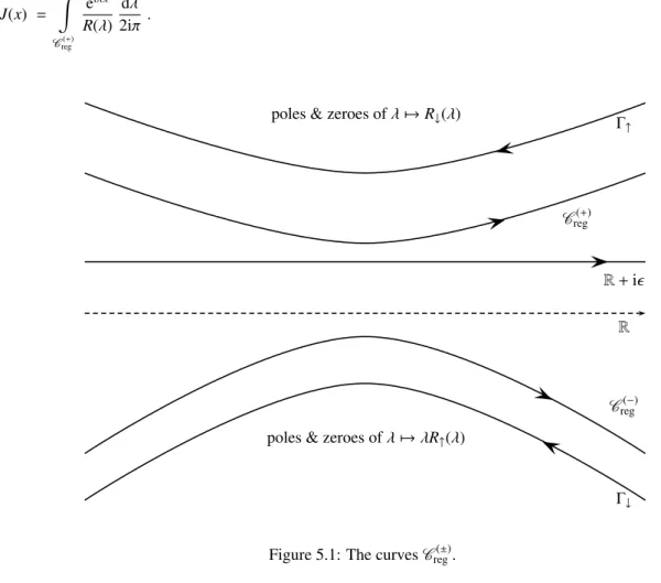
large N-behaviour of the inverse operator: Chapter 5 is devoted to deriving uniform large-N local behaviour for the inverse
operator. Chapter 6 deals with the asymptotic analysis of one and two fold integrals of interest to the problem. In Section 6.1 we build on the results established so far to carry out the large-N asymptotic analysis of single integrals involving the inverse operator. Finally, in Section 6.3 we establish the large-N asymptotic expansion of certain two-fold integrals, a result that is needed so as to obtain the final answer for the expansion of the partition function. The book contains four appendices. In Appendix A we remind some useful results of functional analysis. In Appendix B we establish the asymptotics for the leading order of ln zN[W] by adapting known large deviation techniques. In Appendix C we derive some properties of the
N-dependent equilibrium measures of interest to the analysis. Then, in Appendix D, we derive an exact expression for the
partition functionZN[VG] when β = 1 and VG is a quadratic potential. We also obtain there the large-N asymptotics of
ZN[VG] up to o(1). This result is instrumental in deriving the asymptotic expansion ofZN[V] for more general potential,
since the Gaussian partition function always appears as a factor of the latter. Finally, Appendix E recapitulates all the symbols that appear throughout the book. Some basic notations are also collected in § 1.6.
Acknowledgments
The work of GB is supported by the Max-Planck Gesellschaft and the Simons Foundation. The work of AG is supported by the Simons foundation and the NSF award DMS-1307704. KKK is supported by the centre national de recherche scientifique. His work has been partly financed by the Burgundy region PARI 2013 & 2014 FABER grants ‘Structures et asymptotiques d’intégrales multiples’. KKK also enjoys support from the ANR ‘DIADEMS’ SIMI 1 2010-BLAN-0120-02.
Contents
1 Introduction 7
1.1 Beta ensembles with varying weights . . . 7
1.1.1 Local fluctuations and universality . . . 8
1.1.2 Enumerative geometry and N-fold integrals . . . . 9
1.2 The large-N expansion ofZ(Nβ) . . . 10
1.2.1 Leading order ofZ(Nβ): the equilibrium measure and large deviations . . . 10
1.2.2 Asymptotic expansion of the free energy: from Selberg integral to general potentials . . . 13
1.2.3 Asymptotic expansion of the correlators via Schwinger-Dyson equations . . . 14
1.2.4 The asymptotic expansion of the free energy up to o(1) . . . 20
1.3 Generalisations . . . 21
1.4 β-ensembles with non-varying weights . . . 25
1.5 The integrals issued from the method of quantum separation of variables . . . 26
1.5.1 The quantum separation of variables for the Toda chain . . . 26
1.5.2 Multiple integral representations . . . 29
1.5.3 The goal of the book . . . 31
1.6 Notations and basic definitions . . . 33
2 Main results and strategy of proof 37 2.1 A baby integral as a motivation . . . 37
2.2 The model of interest and the assumptions . . . 38
2.3 Asymptotic expansion of ZN[V] atβ = 1 . . . 39
2.4 The N-dependent equilibrium measure and the master operator . . . 41
2.5 The overall strategy of the proof . . . 44
3 Asymptotic expansion ofln ZN[V] - the Schwinger-Dyson equation approach 47 3.1 A priori estimates for the fluctuations aroundµ(N)eq . . . 47
3.2 The Schwinger-Dyson equations . . . 55
3.3 Asymptotic analysis of the Schwinger-Dyson equations . . . 58
3.4 The large-N asymptotic expansion of ln ZN[V] up to o(1) . . . 64
4 The Riemann–Hilbert approach to the inversion ofSN 67 4.1 A re-writing of the problem . . . 67
4.1.1 A vector Riemann–Hilbert problem . . . 67
4.1.2 A scalar Riemann–Hilbert problem . . . 70
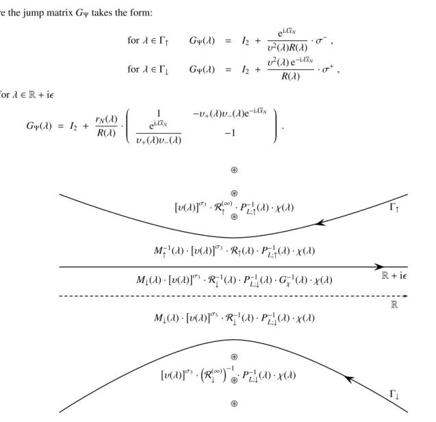
4.2 The auxiliary 2× 2 matrix Riemann–Hilbert problem for χ . . . 72
4.2.1 Formulation and main result . . . 72
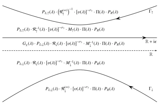
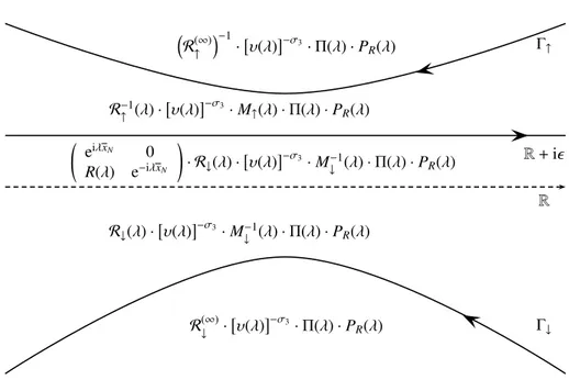
4.2.2 Transformationχ ⇝ Ψ ⇝ Π and solvability of the Riemann–Hilbert problem . . . 72
4.2.3 Properties of the solutionχ . . . 76
4.3 The inverse of the operatorSN . . . 78
4.3.1 SolvingSN;γ[φ] = h for h ∈ Hs([0 ; xN]),−1 < s < 0 . . . 78
4.3.2 Local behaviour of the solution fWϑ[h] at the boundaries . . . 81
4.3.3 A well-behaved inverse operator ofSN;γ . . . 85
4.3.4 WN: the inverse operator ofSN . . . 87
5 The operatorsWNandU−1N 89 5.1 Local behaviour ofWN[H](ξ) in ξ, uniformly in N . . . 89
5.1.1 An appropriate decomposition ofWN . . . 89
5.1.2 Local approximants forWN . . . 94
5.1.3 Large N asymptotics of the approximants ofWN . . . 98
5.2 The operatorUN−1 . . . 103
5.2.1 An integral representation forU−1N . . . 103
5.2.2 Sharp weighted bounds forU−1N . . . 105
6 Asymptotic analysis of integrals 111 6.1 Asymptotic analysis of single integrals . . . 111
6.1.1 Asymptotic analysis of the constraint functionalsXN[H] . . . 111
6.1.2 Asymptotic analysis of simple integrals . . . 114
6.2 The support of the equilibrium measure . . . 117
6.3 Asymptotic evaluation of the double integral . . . 118
6.3.1 The asymptotic expansion related to Id;bkand Id;R . . . 121
6.3.2 Estimation of the remainder∆[k]Id[H, V]. . . 123
6.3.3 Leading asymptotics of the double integral . . . 126
A Several theorems and properties of use to the analysis 129 B Proof of Theorem 2.1.1 131 B.0.4 Partition function and equilibrium measure . . . 136
C Properties of the N-dependent equilibrium measure 139
D The Gaussian potential 143
Chapter 1
Introduction
1.1
Beta ensembles with varying weights
One of the simplest and yet non-trivial example of an N-fold multiple integral that we are interested in is provided by the partition function of aβ-ensemble with varying weights:
Z(β) N [V] = ∫ RN N ∏ a<b |λa− λb|β· N ∏ a=1 e−NV(λa)· dNλ = ∫ RN exp{ ∑ a<b β ln |λa− λb| − N N ∑ a=1 V(λa) } · dNλ . (1.1.1)
β > 0 is a positive parameter and V is a potential growing sufficiently fast at infinity for the integral (1.1.1) to be convergent. Z(β)
N can be interpreted as the partition function of the statistical-mechanical system of N particles at temperatureβ−1, that
interact through a two-body repulsive logarithmic interaction and are placed on the real line in an overall confining potential
V. This logarithmic interaction is the Green function for the Laplacian inR2equipped with its canonical metric. By "varying
weights" we mean that the potential V is preceded by a factor of N, such that the logarithmic repulsion can typically be balanced by the effect of V for λaremaining in a bounded in N interval. This is an important feature of the model that we
shall comment further on. We shall however start the discussion by explaining the origin ofβ-ensembles.
The partition function (1.1.1) can be interpreted as the result of integrating over the spectrum of certain random matrices whose distribution is invariant under one of the classical groups. Consider the real vector spaces:
HN, β=
β = 1 : real symmetricβ = 2 : complex hermitian β = 4 : quaternionic self − dual
N× N matrices.
We denote dM, the product of the Lebesgue measures for the linearly independent real coefficients of such matrices. The Lie groups: GN, β= β = 1 : real orthogonal β = 2 : complex unitary
β = 4 : quaternionic unitary N× N matrices
act onHN, βby conjugation. If M is a random matrix inHN, βdrawn from the distribution‡CN;Ve−Ntr[V(M)]· dM, CN;Vbeing
the normalisation constant, the induced distributionP(Nβ)of eigenvalues must be of the form:
p(Nβ);V(λ)· dNλ with p(N;Vβ) (λ) = 1 Z(β) N [V] N ∏ a<b |λa− λb|β N ∏ a=1 { e−NV(λa)}.
Hence, in this context, the partition functionZ(Nβ)[V] corresponds to the normalisation constant of the induced distribution of eigenvalues. The three casesβ ∈ {1, 2, 4} are very special, since they feature a determinantal or Pfaffian structure that
‡Such distributions are indeed invariant under conjugation byGN, β
is unknown for generalβ. This additional structure allows one to reduce the computation of Z(Nβ)[V] to one of a family of orthogonal or skew-orthogonal polynomials [117].
For generalβ > 0 and polynomial V, the partition function (1.1.1) can also be interpreted as the integral over the spectrum of a family of random tri-diagonal matrices [64, 108], whose entries are independent and have a well-tailored distribution depending on V. As there is no symmetry group acting here, this class of random matrices is very different from the invariant ensembles. It is in nature closer to stochastic Schrödinger operators.
Theβ-ensembles have been extensively studied for more than 20 years, see e.g. the books [5, 51, 117, 131], for two main reasons, that we shall develop below. From the probabilistic perspective, the statistical-mechanics interpretation of β-ensembles makes Z(β)
N [V] and its associated probability distribution a good playground for testing the local universality
of the distribution of repulsive particles [79]. From the perspective of geometry and physics, the interest in theβ = 2 case –viz. random hermitian matrices– has been fostered, since the pioneering works of Brézin-Itzykson-Parisi-Zuber [34], by the insight it provides into two-dimensional quantum gravity and the enumerative geometry of surfaces. This interest was eased by the algebraic miracles that make the caseβ = 2 quite tractable from the computational point of view, and also raised by the desire to understand the geometry (related to the integrable structure associated with the orthogonal polynomials) behind these miracles.
1.1.1
Local fluctuations and universality
The physical idea behind universality is that the logarithmic repulsion dictates the local behaviour of the particles1. The
universality classes should only depend onβ and the local environment of the chosen position on R. Typically one expects that, when N→ +∞, the particles will localise on some union of segments ∪k[ak; bk] and that, up to a O(N−1)precision, the
pthwill localise around a "classical" positionγclp.
To be precise, we introduce the k-point density functionsρ(k)N(x1, . . . , xk). These are symmetric functions of k real variables
characterized (if they exist) by the property that, for any sequence of pairwise disjoint intervals (Ai)ki=1:
PN [ ∃i1, . . . , ik∈ {1, . . . , N} : λij ∈ Aj ] = ∫ A1 · · · ∫ Ak ρ(k)(x 1, . . . , xk) k ∏ i=1 dxi. (1.1.2) ρ(k)
N fails to be a density probability function, because of the unusual normalization:
∫ Rkρ (k) N(x1, . . . , xk) k ∏ i=1 dxi= N! (N− k)!
which follows from (1.1.2) by taking a partition ofR into k pairwise disjoint intervals and symmetrising the integration range. In particular, N−1ρ(1)N(x) is the local mean density of particles.
For instance, ifβ = 2 and we look at intervals of size 1/N around a point x0 ∈ R where the mean density of particles
is smooth and positive – i.e. in the bulk – one expects the distribution of the eigenvalues to converge to the determinantal process of the sine kernel. This means that, if limN→∞N−1ρ(1)N (x0)> 0, we expect that
lim N→∞ ρ(k) N ({ x0+ ξi/ρ(1)N (x0) }k i=1 ) [ρ(1) N(x0) ]k = ρ (k) sin(ξ1, . . . , ξk)
whereρ(k)sinare given by: ρ(k)
sin(ξ1, . . . , ξk)= det1≤i, j≤k
[
Ksin(ξi, ξj)], Ksin(x, y) =
sinπ(x − y)
π(x − y) . (1.1.3)
Still forβ = 2 and if we look at intervals of size 1/N2/3around a point x
0where the mean density vanishes like a square root,
one rather expects to observe the determinantal process of the Airy kernel: ρ(k)
Ai(ξ1, . . . , ξk)= det1≤i, j≤k
[
KAi(xi, xj)], KAi(x, y) =
Ai(x)Ai′(y)− Ai′(x)Ai(y)
x− y . (1.1.4)
1.1. BETA ENSEMBLES WITH VARYING WEIGHTS 9
To reformulate, if the condition:
lim x→x0 limN→∞N−1ρ(1)N (x) √ |x0− x| = A > 0 (1.1.5)
holds, we expect that,
lim N→∞N −k/6ρ(k) N ({ x0+ (πA)2/3N−2/3ξi }k i=1 ) = (πA)−2k/3ρ(k) Ai(ξ1, . . . , ξk).
Without being too precise, let us say that (1.1.5) is the generic behaviour at the edge of the spectrum of random matrices of large sizes.
The expression for the potentially universal distribution of particles for other shapes of large-N local mean density of particles, and other values ofβ are known [144, 132] – although their understanding is currently much more developed for β ∈ {1, 2, 4}. The main theme in universality problems is therefore to prove that given models exhibit these distributions for the local behaviour of particles in the large-N limit. As a matter of fact, the precise mode of convergence to the universal laws that one can obtain is not always optimal from a physical point of view, namely it may hold only once integrated against a class of test functions, or only after integration on intervals of size N−1+ηforη arbitrarily small and independent of N. We refer to the original works cited below to see which mode of convergence they establish.
First results of local universality in the bulk where obtained by Shcherbina and Pastur [130] atβ = 2. Then, at β = 2 and for polynomial V, Deift, Kriechenbauer, McLaughlin, Venakides and Zhou [55] established the local universality in the bulk within the Riemann-Hilbert approach to orthogonal polynomials with orthogonality weight e−NV(x)on the real line. These results were then extended by Deift and Gioev toβ ∈ {1, 2, 4} for the bulk [50] and then for the generic edge [49] universality. The bulk and generic edge universality for generalβ > 0 were recently established by various methods and under weaker assumptions. Bourgade, Erdös and Yau built on relaxation methods so as to establish the bulk [31, 33] and the generic edge [32] universality in the presence of genericCkpotentials. Krishnapur, Rider and Virág [108] proved both universalities by
means of stochastic operator methods and in the presence of convex polynomial potentials. Finally, the bulk universality was also established on the basis of measure transport techniques by Shcherbina [136] in the presence of real-anaytic potentials while universality both at the bulk and generic edge was derived by Bekerman, Figalli and Guionnet [13] forCkpotentials
with k large enough.
1.1.2
Enumerative geometry and N-fold integrals
The motivation to study the all-order asymptotic expansion of lnZ(Nβ)[V] when N→ ∞ initially came from physics and the study of two-dimensional quantum gravity, especially in the caseβ = 2 corresponding to hermitian matrices. In the landmark article [34], Brézin, Itzykson, Parisi and Zuber have argued that, for potentials given by formal series:
V(x)= 1 u (x2 2 + ∑ j≥3 tj j x j)
the free energy lnZ(Nβ)[V] has the formal expansion:
ln( Z (2) N [V] Z(2) N[V|t•=0] ) formal = ∑ g≥0 N2−2gF(g) (1.1.6)
which is to be understood as an equality between formal power series in{tj}, and we use the notation V|t•=0(x) = x
2
2u.
The coefficients F(g)correspond to a weighted enumeration of "maps", i.e. equivalence classes of graphsG embedded in
a topological, connected, compact, oriented surfaceS of genus g such that all connected components Ci of S \ G are
homeomorphic to disks. EachCiwhich is bordered by j edges ofG is counted with a local weight −tj, each vertex inG
is counted with a local weight u, and the overall weight of (G , S ) is computed as the product of all local weights, divided by the number of automorphisms of (G , S ). For instance, choosing t3 , 0 and tj>3 = 0, F(g)enumerates triangulations of
an oriented surface of genus g. More generally, lnZ(Nβ)[V] withβ , 2 gives rise to enumerations of graphs embedded in possibly non-orientable surfaces [73, 119]. Then, the expansion (1.1.6) also contains half-integer g’s. The expansions that had been obtained in [34] and in the many subsequent works in physics that have followed. These handlings were set in the
appropriate framework of providing an equality between formal power series in u and the parameters{tj}j≥3in [70]. Indeed,
the fact of subtracting the free energy of the quadratic potential V|t•(x) = x2/2u in the right-hand side of (1.1.6) turns the
formula into a well-defined equality between formal series; a combinatorial argument based on the computation of the Euler characteristics 2− 2g shows that the coefficient of a given monomial uk∏ℓtℓnℓis given by a sum over finitely many genera g. For a restricted class of potentials†for which the integral (1.1.6) is convergent, the formal power series also corresponds to the N→ ∞ asymptotic expansion of Z(2)N [V]. It is because of such a combinatorial interpretation that these expansions are called "topological expansions", this independently of their formal or asymptotic nature.
The random hermitian matrix model (β = 2) for finite N was also interpreted as a well-defined discretised model of two-dimensional quantum gravity. For fixed{tj}, there is a finite value u = ucat which the model develops a critical point:
the coefficients F(g)exhibit as a singularity of the type (uc− u)(2−γstr)(1−g)with a critical exponent−1/2 ≤ γstr< 0 depending
on the universality class. One of the consequences of the appearance of such singularities is that the average or the variance of the number of faces in a map of fixed genus diverges when u → uc. This allows one to interpret the u→ uclimit as a
continuum limit. In taking such a limit, it becomes particularly interesting to tune the u-parameter in an N-dependent way such that u = uc− N−1+γstr/2· ˜u, hence making each term N2−2gF(g) of order 1 when N → ∞. In such a double scaling
limit, the expansion (1.1.6) does not make sense any more. However, it is expected, and it can be proved in certain cases, that the double scaling limit of the appropriately rescaled partition functionZ(2)N[V] exists. This limit was proposed as a way of defining the partition function of two-dimensional quantum gravity with coupling constant ˜u. We refer to the review [80] for more details. The investigation of these double scaling limits is similar in spirit to the investigation of universality that we already mentioned, with the only difference being that a continuation to complex-valued ˜u does have an interest from the physics point of view, whereas it is often excluded from mathematical study of universality given the difficulty to address it with probabilitistic techniques.
Finally, the all-order expansion (be it formal or asymptotic) of N-fold integrals in theβ-ensembles and generalisations thereof have numerous applications at the interface of algebraic geometry and theoretical physics. The key point is that the coefficients of the all-order expansions have an interesting geometric interpretation, and the study of matrix models in the large N limit can give some insight into topological strings, gauge theories, etc. Describing the exponentially small in N contributions to lnZ(Nβ)[V] has also an interest of its own. It is particularly interesting [115] as a path towards understanding the possible non-perturbative completion(s) of the perturbative physical theories. As an illustration closer to the scope of this book, we shall give in Section 1.3 a non-exhaustive list of N-fold integrals which have a physical or geometrical interpretation.
1.2
The large-N expansion of
Z
(Nβ)1.2.1
Leading order of
Z
(Nβ): the equilibrium measure and large deviations
Given a sufficiently regular potential V growing at x → ±∞ faster than(β + ϵ)ln|x| for some ϵ > 0, the leading asymptotic behaviour of the partition functionZ(Nβ)[V] takes the form :
lnZ(Nβ)[V] = −N2(E(β)[µeq]+ o(1) ) with E(β)[µ] = ∫ V(x) dµ(x) − β ∫ x<y ln|x − y| dµ(x)dµ(y) . (1.2.1)
In these leading asymptotics, the functionalE(β) is evaluated at the so-called equilibrium measureµ
eq, a probability
mea-sure onR that minimises the functional E(β). The notion of equilibrium measure arises in numerous other branches of
mathematical physics, for instance the study of zeroes of families of polynomials or the one of the characterisation of the thermodynamic behaviour at finite temperature of quantum integrable models [63]. The minimiserµeqcan be characterised
within the framework of potential theory [109]. One can show that the equilibrium measure associated with the functional E(β) exists and is unique. We stress thatµ
eqis characterised by (1.2.3) and thus depends onβ only via a rescaling of the
potential, hence imposing the same dependence in the leading order term of the expansion (1.2.1).
Let us explain, on a heuristic level, the mechanism which gives rise to (1.2.1). For this purpose, observe that the integrand
1.2. THE LARGE-NEXPANSION OFZ(Nβ) 11 ofZ(Nβ)[V] can be recast as exp{− N2E(β)[LN(λ)]} where L(Nλ) = 1 N N ∑ a=1 δλa (1.2.2)
is the so-called empirical measure whileδx refers to the Dirac mass at x. For finite but large N, λ 7→ E(β)[L(Nλ)] with
λ1 < · · · < λN attains its minimum at a point γeq = (γeq;1, . . . , γeq;N) whose coordinatesγeq;1 < · · · < γeq;N are bounded,
uniformly in N, from above and below. This minimum results from a balance between the repulsion of the integration variables induced by the logarithmic interaction and the confining nature of the potential V since the entropy is negligible2.
It seems reasonable that the main contribution to the integral, namely the one not including exponentially small corrections, will issue from a small neighbourhood of the pointγeq(or those issuing from permutations of its coordinates) and hence
yield, to the leading order in N, lnZ(Nβ)[V] = −N2(E(β)[L(γeq)
N ]+ o(1)
)
. As a matter of fact, theγeq;aare distributed in such
a way that they densify on some compact subset ofR and in such a way that, in fact, L(γeq)
N converges, in some appropriate
sense, to the probability measureµeq.
This reasoning thus indicates that the leading asymptotics of lnZ(Nβ)[V] issue from a saddle-point like estimation of the integral (1.1.1). This statement can be made precise within the framework of large deviations. Ben Arous and Guionnet [7] showed that the distribution of L(Nλ)under the sequenceP(Nβ)of probability measures associated withZ(Nβ)[V] satisfies a large deviation principle with good rate functionE(β)[µ] at speed N2. This means that, for any open setΩ and any closed set F of
the space of probability measures endowed with the weak topology, we have: lim inf N→∞ N −2lnP(β) N [L (λ) N ∈ Ω] ≥ − infµ∈ΩE (β)[µ] lim sup N→∞ N−2 lnP(Nβ)[L(Nλ)∈ F] ≤ − inf µ∈FE (β)[µ] .
Saying thatE(β)is a good rate functional means that its level sets (E(β))−1([0; M]) are compact for any M ≥ 0. As a direct
consequence of this large deviation principle, the random measure L(Nλ)converges almost surely and in expectation, in the weak topology, towards the (deterministic) equilibrium measureµeq.
The properties of the equilibrium measureµeqhave been extensively studied [53, 109, 133]. Its uniqueness follows comes
from the strict convexity ofE(β). Indeed, given two probability measuresµ
0, µ1and t∈ [0, 1], one has
E(β)[(1− t)µ
0+ tµ1]= (1 − t)E(β)[µ0]+ tE(β)[µ1]− β Q[µ1− µ0]
where, for any signed finite measureν of zero mass, one has: Q[ν] = − ∫ x<y dν(x)dν(y) ln |x − y| = ∫ ∞ 0 dk 2k F[ν](k) 2
which implies thatQ[ν] ≥ 0. Furthermore, it is clear that equality holds if and only if ν = 0. The latter does ensure the strictly convexity ofE(β).
As a solution of a minimisation problem, µeq must satisfy an "Euler-Lagrange equation". This condition states the
existence of a constant Ceqsuch that:
Veff(x)= V(x) − Ceq− β ∫ ln|x − y|dµeq(y), { Veff(x)= 0 µeq−almost everywhere Veff(x)≥ 0 µ−almost everywhere (1.2.3)
where the second condition holds for any probability measureµ on R such that E(β)[µ] < +∞. The inequality comes from the fact that one minimises over positive measures, and the constant Ceqis a Lagrange multiplier for the constraint that the total
mass should be 1. Veff(x) is the effective potential felt by a particle; it takes into account V and the repulsion it feels from
2The Lebesgue measure does not participate to the setting of this equilibrium: the aforementioned terms induce a eO(N2)
behaviour in the light of (1.2.1), while on compact subsets ofRN, the Lebesgue measure produces at most a O(ecN) contribution, with c depending on the size of the compact set.
all other particles distributed according toµeq. The characterisation (1.2.3) expresses that the effective potential is constant
and minimal on the support ofµeq. The constant Ceq is chosen in such a way that this minimum is zero. It thus appears
reasonable to expect that, in the large N limit, the particles should mostly likely accumulate in supp[µeq]. More precisely,
[5, 6, 29] proves a large deviation principle for the position of individual particles at speed N with good rate function Veff.
This means that, for any open subsetΩ and closed subset F of R, we have: lim inf N→∞ N −1lnP(β) N [∃a ∈ {1, . . . , N} λ a ∈ Ω]≥ − inf x∈ΩVeff(x) lim sup N→∞ N−1lnP(Nβ)[∃a ∈ {1, . . . , N}, λa∈ F ] ≤ − inf x∈FVeff(x).
One can prove that if V isCkfor k≥ 2, then µeqis Lebesgue continuous with aCk−2density. Besides, if V is real-analytic,
the density is the square root of an analytic function what, in its turn, implies that its support consists of a finite number of segments, called cuts. Critical points of the model occur when the topology of the support becomes unstable with respect to small perturbations of the potential. Namely when there exist arbitrarily small perturbations of the potential which result in a support of the equilibrium measure in which one of the component has split in two, two components have merged, or where a new cut has appeared†. When this is not the case, one says that the potential is off-critical. For V real-analytic on R, a necessary condition for off-criticality is that µeqvanishes exactly like a square root at the edges of the support:
lim x→a∈∂suppµeq 1 √ |x − a| dµeq dx > 0 and this is the "generic" behaviour. Whenµeqvanishes like|x − a|k+
1
2 with k> 0, a small island of particles around a can separate from the rest and form a new cut under certain small perturbations of the potential.
The simplest example of an equilibrium measure is provided by the one subordinate to a quadratic potential VG(x)= x2.
This equilibrium measure is given by the famous Wigner semi-circle distribution [148]: dµeq(x)= dx βπ · (β − 4x 2)1 2 · 1 [− √ β 2 ; √ β 2] (x)
which has only one cut. Although there is no easy characterisation of the set of potentials V leading to one-cut equilibrium measures, strictly convex V do belong to this set [118]. Indeed, since for any y the function x7→ − ln |x − y| is strictly convex, integrating it over y against the positive measureµeq still gives a convex function. As a result, if V is strictly convex, the
effective potential (1.2.3) is a fortiori strictly convex. This imposes that the minimum of Veffis attained on a connected set,
therefore the support ofµeqis a segment.
A remarkable feature ofβ-ensembles is that, looking at the case of equality in (1.2.3), the density of µeqcan be built
in terms of the solution to a scalar Riemann–Hilbert problem for a piecewise holomorphic function having jumps on the support ofµeq. If one assumes the support to be known, such Riemann–Hilbert problems can be solved explicitly leading to
a one-fold integral representation for the density ofµeq. These manipulations originate in the work of Carleman [37], and
some aspects have also been treated in the book of Tricomi [143]. In the case where the support consists of single segment [a; b] and for V at leastC2, one gets that the density of the equilibrium measure reads:
dµeq(x)= dx · 1[a ;b](x)· b ∫ a dξ πβ · V′(x)− V′(ξ) x− ξ · {(b− x)(x − a) (b− ξ)(ξ − a) }1 2 . (1.2.4)
The above representation still contains two unknown parameters of the minimisation problem: the endpoints a, b of the support ofµeq. These are determined by imposing additional non-linear consistency relations. In the one-cut case discussed
above, the conditions on the endpoints a and b are:
b ∫ a dξ πβ · V′(ξ) { (b− ξ)(ξ − a)}12 = 0, a+ b 2 b ∫ a dξ πβ· ξ V′(ξ) dξ { (b− ξ)(ξ − a)}12 = 1 . (1.2.5)
†Note that under more general deformations of the potential, viz. not necessarily corresponding to small perturbations, it may also happen that two cuts
1.2. THE LARGE-NEXPANSION OFZ(Nβ) 13
The situation, although more involved as regards explicit expressions, is morally the same in the multi-cut case where one has to determine all the endpoints of the support. We stress that the very existence of a one-fold integral representation with a fully explicit integrand tremendously simplifies the analysis, be it in what concerns the description of the properties ofµeq,
or any handling that actually involves the equilibrium measure. The one-cut case is computationally easier to deal with than the multi-cut case: for instant when V is polynomial, the conditions (1.2.5) determining the endpoints a and b are merely algebraic. As we will explain later, there is another, more important difference between the one-cut case and the multi-cut case, that pertains to the nature of the O(1) corrections to the large-N behaviour of the partition functionZ(Nβ)[V].
1.2.2
Asymptotic expansion of the free energy: from Selberg integral to general potentials
For very special potentials, the partition functionZ(Nβ)[V] can be exactly evaluated in terms of a N-fold product. The quadratic potential VG(x)= x2is one of these special cases and the associated partition function is related to the Selberg integral [134],
from where it follows:
Z(β) N [VG] = (2π) N/2· (2N)−N 2(1−β2+β2N)· N ∏ m=1 Γ(1+m2β) Γ(1+β2) .
With such an explicit representation, standard one-dimensional analysis methods lead to the large-N asymptotics of the partition function: lnZ(Nβ)[VG] = {β 4· ln (β 4 ) −3β 8 } · N2+β 2· N ln N + {(1 2+ β 4 ) · ln( β 4e ) +β 2 · ln 2 + ln(2π) − ln Γ ( 1+β 2 )} · N +1 12 ( 3+β 2 + 2 β ) · ln N + χ′(0 ;2 β, 1 ) +ln(2π) 2 + o(1) . (1.2.6)
The functionχ(s ; b1, b2) is the meromorphic continuation in s of the function defined for Re s> 2 by the formula:
χ(s ; b1, b2)= ∑ m1,m2≥0 (m1,m2),(0,0) 1 (m1b1+ m2b2)s .
Note that, whenβ = 2, the constant term in (1.2.6) can be recast in terms of the Riemann zeta function as: χ′(0 ; 1, 1) = ζ′(−1) − ln(2π)
2 .
The o(1) remainder admits an asymptotic expansion in 1/N whose coefficients are expressed as linear combinations with rational coefficients of Bernoulli numbers and 2/β.
For generic potentials V, there is no chance to obtain a simple closed formula forZ(Nβ)[V]. Nevertheless, the cases that are computable in closed form do play a role in the asymptotic analysis of the more generalZ(Nβ)[V] beyond the leading order. Indeed, most of the methods of asymptotic analysis rely, in their final step, on an interpolation between the potential of interest V, and a potential of reference V0 for which the partition function can be exactly computed. The strategy for
obtaining the leading corrections is to conduct, first, a study of the large-N corrections to the macroscopic distribution of eigenvalues, and in particular to the fluctuations of the linear statistics:
EV N [∑N i=1 f (λi)−N ∫ f (x)·dµeq(x) ] = N·EV N [ ∫ f (x)·d(L(Nλ)−µeq)(x) ] ≡ N ∫ RN p(N;Vβ) (λ) { ∫ f (x)·d(L(Nλ)−µeq)(x) ]} ·dNλ (1.2.7)
for a sufficiently large class of test functions f . The subscript V indicates that we are considering the sequence of probability measures for whichZ(Nβ)[V] is the partition function. Assume that one is able to establish the large-N behaviour of (1.2.7) for a one parameter t family{Vt}t∈[0 ;1]of potentials this uniformly in t∈ [0, 1] and up to a O(N−κ−1),κ > 0 and fixed, remainder.
Then one can build on the basic formula:
ln(Z (β) N[V1] Z(β) N[V0] ) = −N2· 1 ∫ 0 EVt N [ ∫ ∂tVt(x)· dL (λ) N (x) ] · dt (1.2.8)
so as to obtain the asymptotic behaviour of the left-hand side up to a O(N−κ) remainder. If by some other means one can access to the large-N asymptotics of lnZ(Nβ)[V0] up to O(N−κ) remainder, then one can deduce the expansion ofZ
(β)
N[V1] to
the same order. The terms of order N ln N, ln N, and the transcendental constant term in the asymptotic expansion of the partition function usually do not arise from the fluctuations of linear statistics, but rather from an "integration constant" or from some additional singularities present in the confining potential. The comparison to some known, Selberg-like integral often seems the only way of accessing to these terms, especially in what concerns the highly non-trivial constant terms in such asymptotic expansions. Note that whenβ = 2 one can build on orthogonal polynomial techniques to access to the
N ln N and ln N terms. Also, recently, some progress in an alternative approach to computing the logarithmic terms has been
achieved in [110].
1.2.3
Asymptotic expansion of the correlators via Schwinger-Dyson equations
As already mentioned, for a general potential, going beyond the leading order demands taking into account the effect of fluctuations of the integration variables around their large-N equilibrium distribution. The most effective way of doing so consists in studying the large-N expansion of the multi-point expectation values of test functions versus the probability measure induced byZ(Nβ)[V], i.e. the quantities:
EV N [ ∫ f (x1, . . . , xn)· n ∏ i=1 dL(Nλ)(xi) ] ,
sometimes called n-linear statistics. Indeed the access to the sufficiently uniform in the potential large-N expansion of the 1-linear statistic allows one to deduce the asymptotic expansion ofZ(Nβ)[V] by means of (1.2.8). As we shall explain in the following, these linear statistics satisfy a tower of equations which allow one to express the n-linear statistics in terms of
k-linear statistics with k≤ n + 1. These equations are usually called the Schwinger-Dyson equations and, sometimes, also
referred to as "loop equations".
We are first going to outline the structure and overall strategy of the large-N analysis of the Schwinger-Dyson equations on the example of a polynomial potential. The latter simplifies some expressions but also allows one to make a connection with the problem of enumerating certain maps. Then, we shall discuss the case of a general potential which will be closer, in spirit, with the techniques developed in the core of the book.
Moments and Stein’s method
For the purpose of this subsection, we shall assume that the potential is a polynomial of even degree Vpol(x)=β2
{x2 2+ ∑2d j=1 tjxj j } with t2d > 0 so that P (β)
N is well-defined. (1.1.6) implies that for any integer number p, the p-th moment
mN(p) := E Vpol N [1 N N ∑ a=1 λp a ] = − 2p βN2∂tplnZ (β) N [ Vpol ]| t•=0. (1.2.9)
has a power series expansion in (tj)2dj=1, whose coefficients enumerate maps (see Section 1.1.2) with one marked face of degree
p. To explain what convergent matrix integrals and their asymptotic expansions on the one hand, and generating series of
maps and their topological decomposition in (inverse) powers of N on the other hand, have to do with each other, we shall use Schwinger-Dyson equations.
Probably, the simplest example of a Schwinger-Dyson equation can be provided by focusing on the standard Gaussian lawγ on R. An integration by parts shows that γ satisfies
∫
x f (x) dγ(x) =
∫
f′(x) dγ(x) . (1.2.10)
for a sufficiently big class of test functions f . In fact, γ is the unique probability measure on R which satisfies (1.2.10). Recall that the pth-moment of the Gaussian law has the combinatorial interpretation of counting the number of pairings of p ordered
points. One can, in fact, build on the above Schwinger-Dyson equation so as to deduce such a combinatorial interpretation by checking that the moments satisfy the same recurrence relation than the enumeration of pairings.
1.2. THE LARGE-NEXPANSION OFZ(Nβ) 15
The strategy to extract the large-N behaviour of moments (1.2.9) relies first on the derivation of the system of Schwinger-Dyson equations they satisfy. As for the Gaussian law, it is obtained by an integration by parts. To write this equation down, we denote by mNthe quenched moments, i.e. the real-valued random variable:
mN(p)= 1 N N ∑ a=1 λp a.
We shall as well adopt the convention that mN(p)= 0 when p < 0. Then, integration by parts readily yields
EVpol N [∑p−1 l=0 mN(l) mN(p− 1 − l) + 1 N (2 β− 1 ) p mN(p− 1) − mN(p+ 1) − 2d ∑ j=1 tjmN(p+ j − 1) ] = 0 . (1.2.11)
Compared to (1.2.10), this equation depends on the dimension parameter N. Note that (1.2.11) not only involves the observ-ables mN = E
Vpol
N [mN], but also the covariance of
{
mN(p)}p≥0. To circumvent this fact, let us assume first that these moments
self-average, so that this covariance is negligible. Let us assume as well that the expectations mN(p) are bounded by some Cp
for some C independent of N, this for all p≤ P(N) where P(N) is some sequence going to infinity with N. Such information imply that the sequence{mN(p)
}
p≥0admits a limit point
{
m(p)}p≥0. Equation (1.2.11) then implies that any such limit point { m(p)}p≥0must satisfy m(p+ 1) = p−1 ∑ l=0 m(l) m(p− 1 − l) − 2d ∑ j=1 tjm(p+ j − 1) . (1.2.12)
Moreover, m(p)≤ Cpfor all p. It is then not hard to see that the limiting equation (1.2.12) has a unique solution such that
m(0)= 1 provided the ti’s are small enough: indeed this is clear for tj= 0 and the result is then obtained by a straightforward
perturbation argument, see [83] for details. Finally, one can check that this unique solution is also given by
M(p)= ∑ ℓ1,...,ℓ2d≥0 {∏2d j=1 (−tj)ℓj ℓj! } Map0(p, ℓ1, . . . , ℓ2d),
where Map0(p, ℓ1, . . . , ℓ2d) is the number of connected planar maps with one marked, rooted face of degree p, andℓjfaces
of degree j, for 1 ≤ j ≤ 2d. Indeed, Tutte surgery – which consists in removing the root edge on the marked face, and describing all the possible maps ensuing from this removal – reveals that these numbers satisfy the recursive relation:
Map0(p+ 1, ℓ1, . . . , ℓ2k) = p−1 ∑ q=1 ∑ ℓj≥lj≥0 {∏2d j=1 ( lj ℓj ) } Map0(q, l1, . . . , l2d)Map0(p− q − 1, ℓ1− l1, . . . , ℓ2d− l2d) + 2d ∑ j=1 ℓjMap0(p+ j − 1, ℓ1, . . . , ℓj−1, ℓj− 1, ℓj+1, . . . , ℓ2d).
which turns into the Schwinger-Dyson equation for the generating function M(p).
This strategy to prove convergence to the generating function of planar maps is very similar to the so-called Stein’s method in classical probability, which is widely used to prove convergence to a Gaussian law. This method can roughly be summarised as follows. One considers a sequence of probability measures{µN}N≥0on the real line and assume that there
exists differential operators{LN}N≥0such that for all N,
µN
[ LN[ f ]
] = 0 for a set of test functions. Assume moreover that{µN
}
N≥0is tight and thatLNconverges towards some operatorL. Then, if
this convergence holds in a sufficiently strong sense, any limit point µ of the sequence{µN}N≥0should satisfy
If moreover there exists a unique probability measureµ satisfying these equations, then this entails the convergence of the sequence{µN}Ntowardsµ. For instance, convergence to the Gaussian law is proved when L[ f ](x) = f′(x)− x f (x). Higher
order of the expansion can be obtained similarly in the case where one knows thatLNadmits an asymptotic expansion:
LN= L +L
(1)
N +
L(2)
N2 + · · ·
so that ifL is invertible one could hope to prove an asymptotic expansion of the form: µN= µ + µ
(1)
N +
µ(2)
N2 + · · ·
at least when integrated against a suitable class of test functions, and with:
µ(1)[ f ]= −µ[L(1)◦ L−1[ f ]], µ(2)[ f ]= −µ(1)[(L(1))2◦ L−1[ f ]]− µ[L(2)◦ L−1[ f ]]. (1.2.13)
The main difference in β ensembles is that the Schwinger-Dyson equation (1.2.11) is not closed on the {mN(p)}p≥0,
namely that involves auxiliary quantities (covariances) which cannot be determined by the equation itself. In order to study the large-N behaviour of the moments by means of the Schwinger-Dyson equation (1.2.11) it is convenient to re-centre the quenched moment around their mean leading to
EVpol N [∑p−1 l=0 ( mN(l)− mN(l) ) ( mN(p− 1 − l) − mN(p− 1 − l) )]− m N(p+ 1) + 1 N (2 β− 1 ) p mN(p− 1) − 2d ∑ j=1 tjmN(p+ j − 1) + p−1 ∑ l=0 mN(l) mN(p− 1 − l) = 0 . (1.2.14)
If one then assumes that the covariance produces o(1/N) contributions and that the moments admit the expansion :
mN(p)= m(p) +
∆mN(p)
N + o(1/N) ,
one would find
Ξ[∆mN](p+ 1) ∼
(2 β− 1
)
p mN(p− 1) ,
whereΞ is the endomorphism of RN, which associates to a sequence{v(p)}p≥0, the new sequence: Ξ[v](p) = v(p) − 2 p−2 ∑ l=0 m(l)v(p− l − 2) + 2d ∑ j=1 tjv(p+ j − 2) . (1.2.15)
When all tj’s are equal to zero,Ξ is represented by a triangular (semi-infinite) matrix with diagonal elements equal to one,
and therefore it is invertible. A perturbation argument shows thatΞ is still invertible when the tj’s are small enough. Hence,
we deduce that lim N→∞∆mN= (2 β− 1 ) pΞ−1[m](p− 1) .
To get the next order of the corrections, one needs to be able to characterise the leading large-N behaviour of the co-variance. To this end, following [2, 3, 40], one derives a "rank 2" Schwinger-Dyson equation, which will give access to the limit of the appropriately rescaled N covariance in the spirit of Stein’s method. This equation is obtained by considering the effect, to the first order in ε, of an infinitesimal perturbation of the potential V(x) → V(x) + εxkin the first Schwinger-Dyson equation (1.2.11), i.e. tj→ tj+ 2δj,kkϵ/β. It results in the insertion of a factor of mN(k) in the expectation value in (1.2.11).
If we introduced the centred random variableemN= N(mN− mN), this "rank 2" equation can be put in the form:
EVpol N [∑p−1 l=0 e mN(k) mN(l) mN(p− 1 − l) − emN(k)Ξ[emN](p+ 1) + 1 N (2 β− 1 ) pmeN(k)meN(p− 1) ] = k mN(k− 1 + p) . (1.2.16)
1.2. THE LARGE-NEXPANSION OFZ(Nβ) 17
In this equation, we simplified some terms exploiting the fact thatemNis centred and that the first Schwinger-Dyson equation
(1.2.11) is satisfied. Again, assuming that the first term in (1.2.16) is negligible, we would deduce that: lim N→∞E Vpol N [e mN(k)emN(p)]= −kΞ−1[Sk−2m](p) := w(k, p) .
where Sk−2m is the sequence whose p-th term is m(k− 2 + p).
Plugging back this limit into the first Schwinger-Dyson equation yields the second order correction:
mN(p)= m(p) + m(1)(p) N + m(2)(p) N2 + o ( 1 N2 ) , with Ξ[m(2)](p+ 1) = p−1 ∑ l=0 { w(l, p − 1 − l) + m(1)(l)m(1)(p− 1 − l)} + (2 β− 1 ) pm(1)(p− 1) .
Again, one can check that whenβ = 2, m(2)is the generating function for maps with genus 1 as its derivatives at the origin
satisfy the same recursion relations, which in the case of maps are derived similarly by Tutte surgery. The same type of arguments can be carried on to all orders in 1/N.
As a summary, to obtain the asymptotic expansion of moments, and hence of the partial derivatives of the partition function c.f. (1.2.9), we see that one needs uniqueness of the solution to the limiting equation (to obtain convergence of the observables), invertibility of the linearised operatorΞ (to solve recursively the linearised equations), a priori estimates on covariances, or more generally of the correlators (in order to be able to get approximately closed linearised equations for the observables). The expansion can then be established and computed recursively, and this recursion is the topological recursion of [75].
The Schwinger-Dyson equations for a general potential
For theβ-ensembles in presence of a general potential V the Schwinger-Dyson equation also arise from an integration by parts. The first Schwinger-Dyson equation takes the form:
EV N [ β 2 ∫ f (x)− f (y) x− y · dL (λ) N (x)· dL (λ) N (y)+ 1 N ( 1−β 2 ) ∫ f′(x)· dL(Nλ)(x)− ∫ V′(x) f (x)· dL(Nλ)(x) ] = 0
Similar equations can be derived for test functions depending on n-variables, although we shall not present them explicitly here. We see that the first Dyson equation relates 1 and 2-linear statistics. More generally, the n-th Schwinger-Dyson equations relates n-linear statistics to k-linear statistics with k ≤ (n + 1). Therefore, as such, the Schwinger-Dyson equations do not allow one for the computation of the n-linear statistics. However, it turns out that these equations are still very useful in extracting the large-N asymptotic expansion of the n-linear statistics. For instance, the leading order as N→ ∞ of the first Schwinger-Dyson provides one with an equation satisfied by the equilibrium measure:
β 2 ∫ f (x)− f (y) x− y · dµeq(x)· dµeq(y) − ∫ V′(x) f (x)· dµeq(x)= 0 . (1.2.17)
This equation is actually implied by differentiating the equality case in the Euler-Lagrange equation (1.2.3) for µeq, and then
integrating the result against f (x)dµeq(x). The most important point, though, is that one can build on the Schwinger-Dyson
equations so as to go beyond the leading order asymptotics. Doing so is achieved by carrying out a bootstrap analysis of the system of Schwinger-Dyson equations. The latter allows one to turn a rough estimate on the (k+ 1)-linear statistics into an improved estimate of the k-th statistics. One repeats such a scheme until reaching the optimal order of magnitude estimates. On the technical level, the essential step of the bootstrap method consists in the inversion of a master operatorK, which appears in the "centring" of the Schwinger-Dyson equation aroundµeq, namely by substituting L(Nλ)= µeq+ L(Nλ)in the first
Schwinger-Dyson equation what, owing to the identity (1.2.17), leads to: EV N [ ∫ K[ f ](x) · dL(λ) N (x)+ β 2 ∫ f (x)− f (y) x− y · dL (λ) N (x)· dL (λ) N (y)+ 1 N ( 1−β 2 ) ∫ f′(x)· dL(Nλ)(x) ] = −1 N ( 1−β 2 ) ∫ f′(x)· dµeq(x) (1.2.18) where: K[ f ](x) = β ∫ f (x)− f (y) x− y · dµeq(y)− V ′(x) f (x)= −V′ eff(x) f (x)− ∫ f (y) x− y · dµeq(y). (1.2.19)
The centred aroundµeqn-th Schwinger-Dyson equations, n≥ 2, all solely involve the operator K.
Now, assuming that the operatorK is invertible on some appropriate functional space, one can recast (1.2.18) in the form
EV N [ ∫ f (x)· dL(Nλ)(x) ] = −1 N ( 1−β 2 ) ∫ ∂xK−1[ f ](x)· dµeq(x) − 1 N ( 1−β 2 ) EV N [ ∫ K−1[ f ]′(x)· dL(λ) N (x) ] −β 2E V N [ ∫ K−1 [ f ](x)− K−1[ f ](y) x− y · dL (λ) N(x)· dL (λ) N (y) ] . The term arising in the first line is deterministic and produces an O(1/N) behaviour. The first term in the second line is given by a 1-linear centred statistic that it preceded by a factor of N−1. It will thus be sub-dominant in respect to the deterministic term. In fact, its contribution to the asymptotic expansion of 1-linear statistics is the easiest to take into account. Indeed, assume that one knows the asymptotic expansion of 1-linear statistics up to O(N−k) and wants to push it one order in N further. Then, the term we are discussing will automatically admit an asymptotic expansion up to O(N−k−1)what readily allows one to identify its contribution to the next order in the expansion of 1-linear statistics. Taken this into account, it follows that the non-trivial part of the large-N expansion of 1-linear statistics will be driven by the one of 2-linear centred statistics. In all cases, if one assumes that the 2-linear statistics produce o(1/N) contributions, the first Schwinger-Dyson equation yields immediately the first term in the large-N expansion of 1-linear statistics. In order to push the expansion further, one should access to the first term in the large-N expansion of 2-linear centred statistics. The latter can be inferred from the second Schwinger-Dyson equation. We shall however, not go into more details.
The main point is that one can push the large-N expansion of k-linear statistics, this to the desired order of precision in N, by picking lower order corrections out of the higher order Schwinger-Dyson equations. The effectiveness of such a bootstrap analysis is due to the particular structure of the Schwinger-Dyson equations. It was indeed discovered in the early 90s that the coefficients of topological expansions in 1/N of the n-point correlators are determined recursively by the Schwinger-Dyson equations. The calculation of the first sub-leading correction to (1.2.1) based on the use of Schwinger-Dyson equations for correlators was first carried out in the seminal papers of Ambjørn, Chekhov and Makeenko [3] and of these authors with Kristjansen [2]. The approach developed in these papers allowed, in principle, for a formal3, order-by-order computation of
the large-N asymptotic behaviour ofZ(2)N [V]. However due to its combinatorial intricacy, the approach was quite complicated to set in practice. In [67], Eynard proposed a rewriting of the solutions of Schwinger-Dyson equations in a geometrically intrinsic form that strongly simplified the structure and intermediate calculations. Chekhov and Eynard then described the corresponding diagrammatics [39], and it led to the emergence of the so-called topological recursion fully developed by Eynard and Orantin in [74, 75]. It allows, in its present setting, for systematic order-by-order calculation of the coefficients arising in the large-N expansions of theβ-ensemble partition functions, just as numerous other instances of multiple integrals, see e.g. the work of Borot, Eynard and Orantin [27]. Eynard, Chekhov, and subsequently these authors with Marchal have developed a similar4 theory [40, 41, 42]. Forβ = 2, Kostov [103] has also developed an interpretation of the coefficient
arising in the large-N expansions as conformal field theory amplitudes for a free boson living on a Riemann surface that is
3Namely based, among other things, on the assumption of the very existence of the asymptotic expansion. 4For potentials with logarithmic singularities andβ , 2, some additional terms must be included [38].
1.2. THE LARGE-NEXPANSION OFZ(Nβ) 19
associated with the equilibrium measure. It was argued in [104] that Kostov’s approach is indeed equivalent to the formalism of the topological recursion.
To summarise, the above works have elucidated the a priori structure of the large N expansions. We have not yet discussed the problem of actually proving the existence of an asymptotic expansion of lnZ(Nβ)[V] to all algebraic orders in
N, namely the fact that
lnZ(Nβ)[V] = c1(β)N ln N+ c(0β)ln N+
K
∑
k=0
N2−kFk(β)[V]+ O(N−K) (1.2.20)
for any K ≥ 0 and with coefficients being some β-dependent functionals of the potential V. The existence and form of the expansion up to o(1) whenβ = 2 was proven by Johansson [92] for polynomial V under the one-cut hypothesis, this by using the machinery described above and a priori bounds for the correlators that were first obtained by Boutet de Monvel, Pastur et Shcherbina [47]. Then, the existence of the all-order asymptotic expansion atβ = 2 was proven by Albeverio, Pastur and Shcherbina [1] by combining Schwinger-Dyson equations and the bounds derived in [47]. In particular, this work proved that the coefficients of the asymptotic expansion coincide with the formal generating series enumerating ribbon graphs of [34] – also known under the name of "maps". Finally, Borot and Guionnet [29] systematised and extended to allβ > 0 the approach of [1], hence establishing the existence of the all-order large-N asymptotic expansion ofZ(Nβ)[V] at arbitraryβ and for analytic potentials under the one-cut hypothesis. This includes, in particular, the analytic convex potentials. The starting point always consists in establishing an a priori estimate for the fluctuations of linear statistics, on the basis of a statistical-mechanical analysis [47] or of concentration of measures [29], without assumptions on the potential beyond a sufficient regularity. This estimate takes the form:
P(β) N [{ λ ∈ RN : ∫ f (x)· d(L(Nλ)− µeq)(x) > t }] ≤ exp{− C[ f ] N2t2+ C′N ln N}
for some constants C[ f ] > 0, C′, and for t large enough independently of N. We remind that if O1, . . . , On are random
variables, their moment is:
EV N [∏n i=1 Oi ] = ∂t1=0· · · ∂tn=0P (β) N [ exp( n ∑ i=1 tiOi )] while their cumulant is defined as:
Cn [ f1, . . . , fn]= ∂t1=0· · · ∂tn=0lnP (β) N [ exp{ n ∑ i=1 tiOi }] .
In fact, the cumulants are enough for computing all the n-linear statistics. Indeed, one has the reconstruction EV N [ ∫ ∏n a=1 fa(xa)· n ∏ i=1 dL(Nλ)(xi) ] = n ∑ s=1 ∑ [[ 1 ; n ]]= J1⊔···⊔Js s ∏ a=1 C|Ja| [{ fk}k∈Ja ].
The expression for n-linear statistics involving genuine test functions in n variables belonging to the test spaceT (Rn) is then
obtained by density of, say,T (R) ⊗ · · · ⊗ T (R) in T (Rn).
It is advantageous to work withCn
[
f1, . . . , fn], since it is a homogeneous polynomial of degree n of the re-centred measure
L(Nλ)− µeq, and concentration occurs in this re-centred measure:
Cn[f1, . . . , fn] ≤ {∏n i=1 N[ fi] } ·(ln N N )n 2
whereN is some norm. Then, under the one-cut assumptions, one shows that the master operator is invertible with a continuous inverse for a suitable normN. These two pieces of information allow one to neglect the contribution of some of the higher order cumulants in the system Schwinger-Dyson equations and lead to a successive improvement of the a priori bounds up to the optimal scale
Cn [ f1, . . . , fn] = 1 Nn−2 { W(0) n [ f1, . . . , fn] + o(1) } . (1.2.21)