Financial crisis forecasts and applications to systematic trading strategies

(1)

HAL Id: tel-01927767

https://tel.archives-ouvertes.fr/tel-01927767

Submitted on 20 Nov 2018

HAL is a multi-disciplinary open access archive for the deposit and dissemination of sci-entific research documents, whether they are pub-lished or not. The documents may come from

L’archive ouverte pluridisciplinaire HAL, est destinée au dépôt et à la diffusion de documents scientifiques de niveau recherche, publiés ou non, émanant des établissements d’enseignement et de

Financial crisis forecasts and applications to systematic

trading strategies

Antoine Kornprobst

To cite this version:

Antoine Kornprobst. Financial crisis forecasts and applications to systematic trading strategies. General Mathematics [math.GM]. Université Panthéon-Sorbonne - Paris I, 2017. English. �NNT : 2017PA01E067�. �tel-01927767�

(2)

UNIVERSIT´

E PARIS I PANTH´

EON-SORBONNE

´

ECOLE DOCTORALE ED-465

CENTRE D’´

ECONOMIE DE LA SORBONNE

Th`

ese

pour obtenir le grade de

DOCTEUR DE L’UNIVERSIT´

E PARIS I

PANTH´

EON-SORBONNE

Spécialité : Mathématiques Appliquées

pr´esent´ee et soutenue par

Antoine Kornprobst

le 23 Octobre 2017

Financial Crisis Forecasts and Applications

to Systematic Trading Strategies

Th`ese dirig´ee par Raphael Douady

JURY :

Michele Benzi Professor, Emory University Rapporteur

Roy Cerqueti Associate Professor, University of Macerata Rapporteur

Christophe Chorro Maitre de Conf´erences HDR, Universit´e Paris I Examinateur

Raphael Douady Chercheur CNRS HDR, Centre d’Economie de la Sorbonne Directeur de th`ese

Hayette Gatfaoui Associate Professor HDR, IESEG School of Management Examinateur

(3)

Acknowledgements

(4)

�� !� �

(5)

Introduction

(6)

The research work presented in my thesis has been articulated around the goal of building financial crisis indicators with the ability to forecast as accurately as possible future market events and then use that information to devise systematic trading strategies. Those financial crisis indicators work from multiple points of view that complement one another. They rely on the correlation and the volatility inside a basked of asset or the components of an equity index, like the SP500 and, in one part of the thesis, we also develop indicators based on the distribution of the spreads of the components of a CDS index, like the Itraxx Europe 125. Those financial crisis indicators are then applied to many different datasets, large and small, and the signal that they provide is used as the basis for the construction of an active trading signal. This thesis is made of three research papers constituting its three chapters. Each of those three papers is, at the date of my defence, about to be independently

submitted or already undergoing review at a peer reviewed publication, albeit

sometimes in a shortened form. The first chapter deals with the construction of two kinds of financial crisis indicators. The first kind of financial crisis indicators is based on the comparison of the empirical spectrum of a rolling covariance matrix to a distribution of reference that may represent either a calm or an agitated market reference. The second kind of financial crisis indicators is based on the computation of the trace or of the spectral radius of the covariance matrix, the correlation matrix or a weighted version of the correlation matrix. The weights that we use in this first chapter are the market capitalization and the volume traded. After defining a total of nine financial crisis indicators, of both kinds, we then proceed to

demonstrate out-of-sample predictive power for one of them, which we choose

to be the spectral radius of the correlation matrix weighted by volume traded applied on our best and most detailed dataset that contains the SP500 index and its stock components. The most interesting aspect of the demonstration of the prediction power of our financial crisis indicator is the implementation of a successful protective put systematic trading strategy based on its signal. While the worth of our approach is demonstrated and the prediction power of our financial crisis indicators clearly established, we also underline the limitations of our approach, which in particular may take the form of a significant number of false positive errors in the signal provided by our financial crisis indicators. The second chapter is constituted of a paper that builds upon the framework and financial crisis indicators constructed in the first chapter. In this second paper, we expands the use of our financial crisis indicators by combining the signals provided by 29 of them and create a decision process designed to govern a portfolio constituted of a mix of cash and ETF shares. Since the main limitation of our financial crisis indicators, while considered individually, is the presence of false positives in their predictions, we aim in this paper at combining the signals provided by many of them and make a systematic trading strategy act on the composition of the portfolio, selling the shares when the risk of a crisis is high and converting the cash into shares when the risk of a crisis is low, only when the indicators reach some kind of consensus in their forecasts. We then apply

(7)

equity indices. The success of the systematic trading strategies based on our financial crisis indicators is demonstrated by comparing their performances to a buy and hold strategy as well as to a large number of paths of a strategy where the choices to convert the cash into shares or the shares into cash is random. The main result in this chapter is the validation of our framework and the demonstration of the usefulness and prediction power of our financial crisis indicators through the production of winning investment strategies based on those financial crisis indicators. The added value of our systematic active strategies, both in comparison to the static buy and hold references and to the random paths is clear in terms of Sharpe ratio, reduced volatility, increased overall performance and Calmar ratio. The third and final chapter talks about another and novel approach to financial crisis indicators, this time by using the dynamic evolution of the distribution of

the spreads of the components of a CDS index, like the Itraxx Europe 125. After

establishing some results that allow us to work with dynamic distributions on solid theoretical ground, we fit the empirical distribution of the spreads of the components of the index with a mixture of two lognormal distributions. From the study of the dynamics of the coefficients of the decomposition of the empirical distribution of the spreads on the basis constituted of the two chosen lognormal distributions, we then build a lower and an upper boundary around the fitted empirical cumulative distribution function of the spreads of the components of the CDS index. This approach defines a Bollinger band around the fitted empirical cumulative distribution function and the crossing of either boundary defining by that band is interpreted in terms of risk and therefore translated into a trading signal. While the establishment of a complete and fully functional active trading strategy using that Bollinger band upper and lower boundary crossing signal is going to be presented in a mature form only in future revisions of this work, the results obtained are still attractive enough to be considered by the asset management industry, to which we believe this work can be extremely useful in order to navigate through a globally uncertain environment.

(8)

Chapter 1

��

�

(9)

An Empirical Approach to Financial Crisis

Indicators Based on Random Matrices

Raphael Douady

1

and Antoine Kornprobst

∗2

1

_{Stony Brook University, Université Paris 1 Panthéon-Sorbonne}

2

_{Université Paris 1 Panthéon Sorbonne, Labex ReFi}

September 5th 2017

Abstract

The aim of this work is to build financial crisis indicators based on spec-tral properties of the dynamics of market data. After choosing an optimal size for a rolling window, the historical market data in this window is seen every trading day as a random matrix from which a covariance and a cor-relation matrix are obtained. The financial crisis indicators that we have built deal with the spectral properties of these covariance and correlation matrices and they are of two kinds. The first one is based on the Hellinger distance, computed between the distribution of the eigenvalues of the empir-ical covariance matrix and the distribution of the eigenvalues of a reference covariance matrix representing either a calm or agitated market. The idea behind this first type of indicators is that when the empirical distribution of the spectrum of the covariance matrix is deviating from the reference in the sense of Hellinger, then a crisis may be forthcoming. The second type of indicators is based on the study of the spectral radius and the trace of the covariance and correlation matrices as a mean to directly study the volatil-ity and correlations inside the market. The idea behind the second type of indicators is the fact that large eigenvalues are a sign of dynamic instability. The predictive power of the financial crisis indicators in this framework is then demonstrated, in particular by using them as decision-making tools in a protective-put strategy.

Keywords: Quantitative Finance, Econometrics, Simulation Methods, Fore-casting, Large Data Sets, Financial Crises, Random Matrix Theory

(10)

1 Introduction

The objective of this paper is to build financial crisis indicators capable of pro-ducing a useful forecast of future market events. The goal that we set for this study is not to predict the actual occurrence of financial crises. What we aim to achieve is rather to be able to evaluate at a given date whether the probability of a financial crisis happening at the given time horizon is getting higher, because the market conditions are ripe for a random adverse event from inside or even outside the market, to trigger a destructive chain reaction. Examples of random events capable of triggering a financial crisis are many. It may take the form of the sudden failure of a critical company, the publishing of new macro-economic data, a sovereign state defaulting on its debt, a major political event or even a terrorist attack. To use an analogy, we do not pretend to be able to predict the exact moment when a random spark will ignite the gas in the room, but we can measure whether the gas concentration in the room is just right for a random spark to cause a disaster. Since random adverse events happen all the time, measuring whether the conditions are just right in the market for one such event to trigger a crisis should be statistically equivalent to forecasting the actual occurrence of

ﬁ_{nancial crises.}

We build nine original financial crisis indicators which are divided into two kinds: those that study the distribution of the whole spectrum of the covariance matrix and compare it to a reference distribution and those that compute a spe-cific spectral property (namely the trace and the spectral radius) of the covariance, correlation and weighted correlation matrix. Both kinds of indicators rely on the study of the underlying correlation and volatility signals inside the market. This is a novel approach because, while many different kinds of financial crisis indicators do exist in the literature, we are not aware of any that use reference distributions to compare the empirical spectrum of the covariance matrix to, nor any that use a modified version of the correlation matrix where the assets have been weighted with respect to the market capitalization of the corresponding companies or the daily traded volume. This approach enables us to maximize the amount of infor-mation coming from the market that is used by the financial crisis indicators, with the goal of boosting their predictive power. We work with seven datasets, each one designed with its own unique composition characteristics. This provides us with original results about many different financial markets from North America to emerging countries.

There is a large literature on ﬁnancial crisis forecasting, especially works by Sornette (2009), Sornette and Johansen (2010) , Jiang et al. (2010) and Maltritz (2010) , which aim at producing a comprehensive model comprising the genesis,

(11)

dynamics and eventual prediction of financial crises, especially using the powerful tools of time-series analysis. Network theory has also been successfully applied to financial crisis forecasting and the building of financial crisis indicators as in Celik and Karatepe (2007) or Niemira and Saaty (2004). A machine learning approach, based on K-means clustering, to forecasting financial turmoil, and espe-cially sovereign debt crises, has been developed in Fuertes and Kalotychou (2007) who also demonstrated that combining multiple forecasting methods improves the quality of the predictions, as Clemen (1989) had underlined in a review and anno-tated bibliography about combining forecasts. Cross sectional time series analysis in a panel data framework was studied in Van den Berg et al. (2008) to predict

ﬁ_{nancial crises while Bussiere and Fratzscher (2006) chose to develop early}

warn-ing systems of ﬁnancial crises based on a multinomial logit model. Demyanyk and Hasan (2010) summarized the results provided by several prediction methods of

ﬁ_{nancial crises, and especially bank failures, based on economic analysis,}

opera-tions research and decision theory, while Drehmann and Juselius (2014) proposed detailed evaluation criteria of the performance of early warning indicators of bank-ing crises. Financial crisis forecasts can also be based on the quantitative study

of any kind of qualitative macro-economic data like the FOMC 1 _{minutes, or any}

other qualitative forecasts. That approach was developed by Stekler and Syming-ton (2016) as well as Ericsson (2016). Its main limitation resides in the quality of the qualitative forecasts and the FOMC for example did not predict the 2007-2008

ﬁ_{nancial crisis in advance nor did it identify it quickly as a major systemic event.}

From another point of view, Guégan (2008) used chaos theory and data filtering techniques to make market forecasts. The approach that we adopt is more modest in the sense that we do not pretend to explain the precise macro-economic mech-anism that creates the many different kinds of financial crises and to predict the precise date of the next crisis. The ambition of this work is merely to detect a heightened risk of a crisis happening, not to predict its actual occurrence. The approach we adopt is closer to the work of Sandoval Junior and De Paula Franca (2012) who proved in their paper, using random matrix theory techniques, that high volatility in financial markets is intimately linked to strong correlations be-tween those financial markets.

Nonetheless, Sandoval Junior and De Paula Franca only used the Marchenko Pastur distribution in their work, while we intend to build and use additional dis-tributions in the framework of random matrix theory. We also address internal correlations within the ﬁnancial markets and not just the correlations between market indices. Those new distributions are numerically computed as closed form

1

Federal Open Market Committee, which is the branch of the Federal Reserve Board that determines the direction of monetary policy

(12)

formulas for them do not exist to our knowledge. They are introduced in order to escape the restrictive framework of Marchenko-Pastur’s theorem, which assumes uncorrelated Gaussian components. Indeed, the empirical covariance matrix of assets inside a market in turmoil is dominated by strong correlation and a non-Gaussian distribution of the log-returns. Of course, the objectives of this study are also very different, since we attempt to build empirical financial crisis indicators, which are almost ready for use by practitioners, while Sandoval Junior and De Paula Franca were concerned with proving a result about volatility and correla-tion reinforcing their effects during a financial crisis.

The approach and methods used in this study are also close to the work of Bouchaud, Potters and Laloux (2005 and 2009). Indeed, in their 2005 physics pa-per and 2009 review, they apply random matrix theory and principal component analysis to the ﬁnancial context in order to anticipate market events and produce optimal portfolio allocations as well as risk estimations. Their idea to use, like Sandoval Junior and De Paula Franca, the Marchenko Pastur distribution as a reference distribution to which they compare empirical spectra is similar to the framework that we have developed but they use an exponentially weighted moving averages in place of the rolling matrix that we work with. The work of Singh and Xu (2013) and of Snarska (2007) about the dynamics of the covariance matrix in a random matrix theory framework was also inspirational to us. Indeed, the approach we select uses as well rolling windows for dynamic correlation and covari-ance matrices. Exploiting the spectra of those matrices forms the very foundation of the framework of this study.

We can also see the financial crisis indicators that we build as market instability indicators. Indeed, they are able to say at a given date whether the probability of occurrence of a financial crisis within a given time horizon has increased, while it is still possible that the probability of nothing happening remains very high. In particular, one possible limitation of our approach is the relatively high ratio of false positives. There is still usually a high probability that nothing will happen, even when the indicators return red flags. From a practitioner’s point of view, the information that the probability of a crisis occurring in the near future has risen from, say, 0.1% to 10% has tremendous value, even though there is still a 90% chance of nothing happening. For us, a financial crisis indicator is a tool that makes use of publicly available data to determine whether the market conditions, measured by taking into account both correlation and volatility, are ripe in the market for a crisis event to happen.

(13)

fi_{nancial economics: when correlations between asset returns increase and develop} abnormal patterns, when volatility goes up, then something is not right inside the market and a financial crisis event might be around the corner. Any kind of market data can be used within the framework that we created. Depending on the order of magnitude and scope of the financial crises that we intend to forecast, we have the freedom to choose the geographical characteristics of the data. Indeed, we can use prices time series restricted to assets located in one given country, one region or the whole world. The nature of the data can also be freely defined depending on the nature of the crisis events that we plan on forecasting. Stock prices and equity index prices, as well as sector indices may be used to forecast stock market crashes. Foreign exchange (FX) spreads may be used to forecast primarily monetary crises, and the methods that we develop provide a complementary point of view to the work of Guégan and Ielpo (2011) who used time-series models to forecast mon-etary policy. However, we are not limited to any asset class. We may also use bond yields, commodity prices or credit default swaps (CDS) spreads. Finally, it is possible to choose the frequency of the data and adapt it to reflect the kind and scope of the financial crises that we aim at forecasting, the only limitation being data availability.

In this paper, we chose to mainly focus on global ﬁnancial crises, most of which

are well known to the general public and the he data 2 _{has been selected}

accord-ingly. The code has been written using Matlab and its various optional toolboxes . The reader is very much encouraged to apply the methods developed in this paper to their own datasets and to verify the reproducibility of their forecasting power to various kinds and scopes of ﬁnancial crises using data from many diﬀerent kinds of asset classes and of various frequencies. We look forward to feedback and comments.

We propose in this paper a new approach regarding early warning financial crisis indicators that we then illustrate using many different datasets of market data. We also demonstrate the ability of the methods that we develop to make out-of-sample predictions. From our point of view, it seems that no such work has been published before with the same objectives and methodology. Therefore, we cannot compare quantitatively in terms of accuracy and predictive power the results that we have obtained to other existing studies. The work of Bouchaud, Potters and Laloux (2005 and 2009) uses a methodology that is similar to the one we chose, however we did not find detailed empirical results for their work, that would have been suitable for comparison in a robust way with the numerical results that we have obtained in this study.

2

(14)

Besides the present introduction and a general conclusion, the paper is di-vided into four parts. We first describe how we built, collected and processed the databases. Indeed, their quality and diversity constitutes a major part of the interest of the study we conducted. In a second part, we detail the methodology and then we build the financial crisis indicators. The third part is dedicated to the qualitative analysis of the results provided by the financial crisis indicators over the whole length of the datasets. Finally, in the fourth part, we demonstrate the predictive power of the approach we developed by selecting two of the best per-forming financial crisis indicators applied to the largest and most detailed dataset that we possess. After dividing the data between an in-sample and an out-of-sample period, we study in details the forecasting possibilities they provide, firstly by using fixed dates of known financial crises and then by quantitatively defining a

ﬁ_{nancial crisis in terms of the crossing of a chosen maximum draw down threshold.}

2 The Data

The data is constituted at each date of the log-returns with respect to the previous trading day, computed from open or close prices. The prices have been adjusted for dividends and splits beforehand. We have chosen daily data for this study because of easy access and faster numerical handling. Further studies may explore higher frequency data. The model that we develop requires the choice of a rolling window in order to compute the financial crisis indicators. In order to limit aver-aging effects and to have financial crisis indicators with enough responsiveness to provide useful information to a practitioner, we chose the size of the rolling window to be 150 days in the past. This represents roughly six months of trading since we only take trading days into account. Using a relatively large rolling window means that the covariance matrix will be degenerate sometimes since there will be more observations than assets. This fact however is not going to be a problem because for the first type of indicators, the distance between the empirical distribution and the reference will be computed after truncating the empirical distribution around zero and making it stick to the reference in order to eliminate the contribution of the small eigenvalues. The motivations for this operation will be explained in the next section where the methodology that we use is explained in detail. For the second type of indicators, the presence of zeros, even quite a lot of them, in the spectrum will not change anything for the computation of the trace and spectral radius.

Seven datasets, each designed with its own unique properties and composition are considered in this study :

(15)

• The first dataset (Dataset 1) is constituted of eleven stock indices represen-tative of the Asian, European and American financial markets in order to obtain a picture of the global financial system. It is a pure equity dataset that is designed to capture contagion between major financial markets as a way to forecast financial crises. It contains the Nikkei225 (NKY, Japan), Hang Seng (HSI, Hong-Kong/China), Taiwan Stock Exchange Weighted In-dex (TWSE, Taiwan) for the Asian market, the DAX30 (DAX, Germany), FTSE100 (UKX, U.K), IBEX35 (IBX, Spain) for the European market, the SP500 (SPX, U.S.A), Russel3000 (RAY, U.S.A), NASDAQ (CCMP, U.S.A), Dow Jones Industrial Average (INDU, U.S.A), SP/TSX Composite Index (SPTSX, Canada) for the North American market. Dataset 1 spans from January 7th 1987 to February 5th 2015. In order to avoid contaminating the data with time differences which might create bias and spurious correlations, we matched at a same date t the close price in Asia at t, the close price in Europe at t and the open price in America (East Coast) at t. In the absence of intraday data, this appeared to be a reasonable choice. We considered only the trading days and because of the different holidays specific to each of the three markets considered (Asian, European and North American) and the requirement to keep only the trading days that were common to all the markets, the 252 trading days a year have been reduced to around 200 dates. Comparison with the other datasets (particularly Dataset 3 and Dataset 4 below which do have around 250 entries a year since they are exclusively American and European, respectively) shows that this is not a major issue in practice.

• The second dataset (Dataset 2) is constituted of sixteen assets. It contains all of the indices of Dataset 1, some commodity indices and some safe haven or cash equivalent securities toward which investors tend to turn in a time of crisis or impending crisis. It spans the same period as Dataset 1, from Jan-uary 7th 1987 to FebrJan-uary 5th 2015. The treatment of the data with regard to time diﬀerences between geographical regions and non-trading days is the same. On top of the content of Dataset 1, Dataset 2 includes: The Lon-don Gold Market Fixing Index (GOLDLNPM, U.K), the Philadelphia Stock Exchange Gold and Silver Index (XAU, U.S.A), Oppenheimer Limited-Term Government Fund Class A (OPGVX, U.S.A), Sugar Generic Future Contract (SB1, U.S.A), generic First Crude Oil WTI (CL1, U.S.A). The inclusion of precious metal indices, cash equivalent short-government monetary funds, representative agricultural as well as energy commodities (in the form of in-vestable futures) is supposed to provide a longer fuse to the ﬁnancial crisis indicators. As a matter of fact, when the market starts to overheat, investors may liquidate some of their equity positions but they will have to re-invest

(16)

the cash somewhere and those cash equivalent securities are here to account for that. Since those safer, cash equivalent securities are in Dataset 2, we an-ticipate that the risk of a crisis happening will be detected sooner. Moreover, when the market is becoming unstable, one typically witnesses an increase in the correlations between commodity and energy securities (typically large oil companies stocks included in the indices). Since we included some investable commodity futures (like oil futures) in Dataset 2, we expect to capture that eﬀect which is indicative of the appearance inside the ﬁnancial market of the right conditions for a crisis to happen.

• The third dataset (Dataset 3) contains twelve assets which are the SP500 in-dex and its ten sector sub-indices (consumer discretionary, consumer staples, energy, financials, health care, industrials, information technology, materials, telecommunication services, utilities) plus a small capitalization index, the Russel 2000. This dataset should provide information about the inner work-ings of the SP500 and enable us to detect "American" crises (for example the Sub-Prime Crisis of 2007) sooner and with a higher precision than Dataset 1 or Dataset 2 which are global by design and include information about the contagion between the three largest financial markets (Asia, Europe, North America). However, since the North American market still leads the world of finance, it is to be expected that the actual crises anticipated by the use of either three of Dataset 1, Dataset 2 or Dataset 3 will be roughly the same. The inclusion in the mix of a small capitalization index is to try to take advantage of the fact that in the times leading up to a financial crisis, the small caps tend to overheat and form speculative bubbles while they become more and more correlated between themselves and stocks with larger market capitalization. Dataset 3 spans from September 13th 1989 to December 27th 2013.

• The fourth dataset (Dataset 4) is the European counterpart of Dataset 3. It contains eleven assets : the Bloomberg European 500 Index (BE500) and its ten sector sub-indices, which are the same as for the SP500 (consumer discretionary, consumer staples, energy, financials, health care, industrials, information technology, materials, telecommunication services, utilities). As we did not find any European-wide equivalent to the Russel 2000, it does not include small caps however. It should enable us to better and sooner detect "European" crises like the E.U Sovereign Debt Crisis of 2010 while still containing enough information to detect all the other global financial crises. It spans from January 1st 1987 to December 27th 2013.

• The fifth dataset (Dataset 5) is designed with the financial concept of flight

(17)

anxiety of market agents is building up and they tend to abandon equity positions in favor of safer investment grade treasury or corporate bonds. In that regard, the usual observed phenomenon is a positive correlation between equity and bonds in a bull market and a negative correlation between equity and bonds in a bear market. When the correlation between equity and bonds is becoming too high, this may be a sign that the bull market is about to burn itself out, that a bubble is about to burst, heralding the start of a

ﬁ_{nancial crisis. Dataset 5 is built with the detection of that phenomenon in}

mind. It contains all of the data of Dataset 3 (SP500 index, its 10 sector indices and the Russel 2000 as a small capitalization index) plus a number of funds based on investment grade sovereign or corporate bonds. Much like Dataset 3, Dataset 5 is U.S market oriented and is therefore more suited to anticipate crises that originate from or directly aﬀect the North American market. For the long government bonds we have : Wasatch-Hoisington U.S. Treasury Fund (WHOSX) and Thornburg Limited Term U.S. Government Fund Class A (LTUCX). For the corporate bonds we have selected Lord Abbett Bond Debenture Fund Class A (LBNDX) and Vanguard Long-Term Investment-Grade Fund Investor Shares (VWESX) which have both enough AUM (Assets Under Management) to be systemically signiﬁcant and have existed for a long enough time to be historically relevant. Dataset 5 contains therefore 16 assets and spans from September 13th 1989 to December 27th 2013.

• The sixth dataset (Dataset 6) is constituted of 226 individual components of the SP500 index. Because of the evolution over time in the composition of the index, a balance had to be found between keeping a sufficient number of components and having enough historical data. It spans from January 17th 1990 to May 15th 2015. The Apple Inc (AAPL) stock was chosen as the ref-erence with regard to filtering out non-trading days and whenever another element of data was unavailable (on rare seemingly random days it appears that some individual stocks were not traded or the data was unavailable) we carried over the last previously available value. We assumed that this manip-ulation would not compromise the overall quality of the data. Besides those considerations, a few stocks like for example Range Resources Corporation (RRC UN) and The Charles Schwab Corporation (SHCW UN) presented significant data gaps and were removed from the dataset. Since building a dataset with exactly 500 components of the SP500, taking in account the evolution in the composition of the index over time, proved an impossible task due to its complexity and the availability of the data (mergers, corpo-rate spin-offs and private equity acquisitions would have had to be taken into considerations as well), we are aware of the fact that Dataset 6, especially

(18)

when used in conjunction with financial crises indicators might suffer from survivorship bias. As a matter of fact, especially in the times leading up to a crisis, the failing companies drop below the capitalization threshold or are acquired by others while new healthier firms enter the index. We built Dataset 6 because, as we are going to see in the empirical section, working with whole indices and/or limited number of individual securities like in all the previous datasets we created (especially Dataset 3 which resembles a scaled down version of Dataset 6), tends to have an averaging effect on the correlations and renders the correlation signal too noisy and blurred to be useful as a crisis detection method. For reference, the Bloomberg tickers of all the stocks inside Dataset 6 are provided in appendix. Besides the daily close price, from which we derive the log-returns, that is contained in all the other datasets, Dataset 6 also includes daily volumes and market capitaliza-tion. Those extra variables will enable us later to add appropriate weights to the individual stocks in order to refine the computation of the indicators. • The seventh dataset (Dataset 7) is constituted of the SP500, the Russel 2000 index and ten indices from emerging markets : Buenos Aires Stock Exchange Merval Index (MERVAL, Argentina), Ibovespa Brasil Sao Paulo Stock Ex-change Index (IBOV, Brasil), Mexican Stock ExEx-change Index (MEXBOL, Mexico), Moscow Exchange Composite Index (MICEX, Russia), Hong Kong Hang Seng Index (HSI, Hong Kong/China), Shanghai Stock Exchange Com-posite Index (SHCOMP, China), Jakarta Stock Exchange ComCom-posite Index (JCI, Indonesia), National Stock Exchange CNX Nifty Index (NIFTY, In-dia), FTSE/JSE Africa All Share Index (JALSH, South Africa), Borsa Is-tanbul 100 Index (XU100, Turkey). It spans from September 22nd 1997 to May 12th 2015. The relatively shallow depth of this dataset, which in particular may render the study of the Asian crisis of the late 1990’ more difficult, is due to gaps in data availability, especially for the Russian index that we decided to keep anyway due to its importance for the global com-modity and energy markets. All those emerging indices were expressed in the local currency on Bloomberg and were therefore converted into U.S dollars. This conversion was very important when dealing with emerging economies where the exchange rate of the local currency against the U.S dollar can

ﬂ_{uctuate wildly and violently especially in the times leading up to, and}

dur-ing a ﬁnancial crisis. Unlike in advanced economies (we did not convert the European and Japanese indices into U.S dollars in Dataset 1 for example), the position of the currency of an emerging country against the U.S dollar is also highly correlated to the health of the local real economy. This idea was developed by Hawkins and Klau (2000) when they were working with the Bank of International Settlements: in emerging markets, ﬁnancial crises are

(19)

often preceded by overvalued exchange rates and inadequate international monetary reserves.

Regarding the selection of the financial crisis events on a global scale (for use mainly with Dataset 1 and Dataset 2) or at least a regional scale (for use mainly with Dataset 3, Dataset 4, Dataset 5, Dataset 6 and Dataset 7) of the last 30 years, we compiled Table 1 below, which has no ambition of being exhaustive. Succinct historical context will be discussed in the empirical results section when needed. While categorizing the various kinds of financial crises goes far beyond the scope of this paper, we strove to consider a wide selection in the kinds of crises. There are stock market crashes like Black Monday in 1987 and the NASDAQ Crash in 2000. There are financial crises that are rooted into a deep structural fragility of some parts of the real economy, like the real estate sector in the case of the Japanese Asset Price Bubble of the early 1990’ and the Sub-prime Crisis that started in America during the summer of 2007 or the automobile industry in the case of the bankruptcy of General Motors in June 2009, four years after Delphi Corporation, which was General Motors’ main supplier of automotive parts. There are financial crises for which the main trigger was a sovereign debt default like the Russian crisis in 1998, the Argentine crisis in 2001 or the Eurozone crisis, triggered by the Greek haircut in 2010. There are monetary crises as well, like Black Wednesday in 1992 when the British government was forced to withdraw the Pound Sterling from the European Exchange Rate Mechanism (ERM) or the Mexican crisis triggered by the devaluation of the peso against the U.S Dollar. Since none of the datasets include foreign exchange data, we do not expect that any of the indicators will perform well when it comes to anticipating monetary crises, however. There are banking crises as well such as the S&L crisis in America that spanned from the mid-1980’ to the mid-1990’ and during which almost one third of all American savings and loans associations (financial institutions that are allowed to accept savings deposits and to make loans) failed, including hundreds of banks of all sizes and systemic significance. The dates chosen may sometimes seem a little arbitrary but choices had to be made, especially for crises that, unlike Black Monday that played out mostly within a few days of extreme market distress, took place over many months or even years of sustained drop like the NASDAQ in early 2000, which took nearly four months to lose almost two fifth of its March 10th peak. Most financial crises do not happen in one day and instead result from a long process of instability buildup inside the market, the kind of which the indicators that we have built are detecting. When a crisis is best described by a clear ex-plosion, then the date of that event was chosen (Black Monday, the day Lehman Brothers failed, etc...). When a date for a crisis spanning months or years had to be chosen for this study, we considered either the date of the most marking event (the day the NASDAQ peaked, the day General Motors filled for Chapter 11

(20)

bankruptcy3, the day the Greek haircut was announced, etc...) or a date roughly situated in the middle of the crisis process like January 1st 1990 for the S&L crisis.

Date (Y/M/D) Name

1987-10-19 Crisis 1 : Black Monday

1990-01-01 Crisis 2 : S&L Crisis

1990-08-01 Crisis 3 : Japanese Asset Prices Bubble Burst

1991-09-19 Crisis 4 : Scandinavian Banking Crisis

1992-09-16 Crisis 5 : Black Wednesday

1994-12-20 Crisis 6 : Mexican Crisis

1997-07-25 Crisis 7 : Asian Crisis

1998-08-17 Crisis 8 : Russian Crisis

2000-03-10 Crisis 9 : NASDAQ Crash (dot-com Bubble)

2001-02-19 Crisis 10 : Turkish Crisis

2001-09-11 Crisis 11 : 911 Attacks

2001-12-27 Crisis 12 : Argentine Default

2005-10-08 Crisis 13 : Delphi (G.M) Bankruptcy

2007-07-01 Crisis 14 : Sub-prime Crisis

2008-09-15 Crisis 15 : Lehman Brothers Collapse

2009-06-01 Crisis 16 : General Motors Bankruptcy

2010-04-23 Crisis 17 : European Sovereign Crisis

2011-08-05 Crisis 18 : US Sovereign Credit Degradation

2014-12-16 Crisis 19 : Russian Financial Crisis

(Table 1: Selection of Financial Crisis Events in the past 30 years)

3 Methodology

Using the seven datasets that we have built, the methodology is based on the use of the spectrum of the covariance matrix, the correlation matrix and a weighted version of the correlation matrix. At each date, for a sequence of rolling windows, we either compare the whole spectrum to three reference distributions detailed below (two of the reference distributions characterize a calm market and a third one represents a market in turmoil), which gives us the indicators of the ﬁrst kind, or we merely compute the spectral radius and the trace, which gives us the indicators of the second kind. We now details this methodology using Matlab’s formalism and vector indexing conventions.

3

Chapter 11 of Title 11 of the United States Code (also known as the United States Bankruptcy Code) which permits reorganization. In contrast, Chapter 7 provides a legal frame-work for liquidation.

(21)

3.1 Framework

We decided to consider a rolling window T of 150 days in the past at each date and for all datasets, irrespective of the number N of assets they contain. This choice provides us with a good balance between the readability of the signals, favored by a longer rolling window because of the averaging eﬀect, and the responsiveness of the indicators, favored by a shorter rolling window.

For each of the seven datasets, we build at each date t a rolling window ROL(t) of length T . Then, we compute the rolling covariance matrix CV (t) and the rolling correlation matrix CR(t) by using the following formulas written for every row (i.e asset) j œ J1, NK: ROLú (t)(j, :) = ROL(t)(j, :) ≠ mean(ROL(t)(j, :)) (1) CV (t) = 1 T.ROL ú (t) ◊ (ROLú (t))Õ (2) CR(t)(j, :) = ROL ú_{(t)(j, :)} Ò var(ROL(t)(j, :)) (3)

While working with a covariance matrix instead of a correlation matrix, we of course have to rescale the eigenvalues of CV (t). We perform this either by notic-ing that the standard deviation of ﬁnancial log-returns is typically in the order of magnitude of a few percents (a œ [0.01, 0.03]) and therefore multiplying the

eigenvalues by _a12, or by computing the mean of the variances of all the complete

time-series in advance and multiplying by the inverse of that value (for example, we ﬁnd a rescaling factor of 3410 for Dataset 2). This is what we decided to do but it should not be considered as a violation of the measurability of the indicators with respect to the natural time ﬁltration (i.e knowledge of the future). It is just a practical way of rescaling by choosing the most appropriate value and it could just as well have been obtained from historical data predating the sample.

With regard to the reference distributions we use for the ﬁrst type of indicators, we have built three of them :

• Θ1: the theoretical Marchenko Pastur distribution. It is derived from Marchenko Pastur’s theorem presented in the work of Marchenko and Pastur (1967). Let

X be a N ◊ T random matrix of i.i.d normal N (0, ‡2_{) coeﬃcients (in this}

study, each row represents an asset and each column represents an observa-tion at a date t), then when N, T ≠æ Œ and the aspect ratio of the matrix, N/T ≠æ “ < Œ, then the distribution of the eigenvalues of the covariance

(22)

below. This formula (6) below is supposed to be valid for 0 < “ < 1, oth-erwise in the degenerate case, an atom at zero has to be added, but since we intend to truncate the computation of the Hellinger distance to exclude the very small eigenvalues, as we will explain in the next section, this is the formula we are going to use anyway for simplicity.

⁄+= ‡2(1 +Ô“)2 (4) ⁄≠ = ‡2(1 ≠Ô“)2 (5) f (x) = 1 2ﬁ‡2_“ Ò (⁄+ ≠ x)(x ≠ ⁄≠) x 1[⁄≠,⁄+] (6)

The Marchenko Pastur distribution also provides thresholds ⁄+ _{and ⁄}≠

that we use even while working with other simulated reference distributions. Be-cause of the stringent theoretical requirements of Marchenko Pastur’s the-orem, that will never be even remotely satisfied by real financial data, the Marchenko Pastur distribution has no vocation to be the best distribution fulfilling the role of a calm market reference, but it is still going to be useful in this study.

• Θ2: the distribution of the eigenvalues of the covariance matrix of a simu-lated random matrix made of Gaussian N (0, 1) coeﬃcients where the as-sets, materialized as the rows, present some correlation to one another. Let

us consider a rolling matrix (Zi,j)(i,j)œJ0,N K◊J0,T K, containing T observations

(columns) and N assets (rows) and constituted of i.i.d Gaussian N (0, 1) coeﬃcients. We introduce correlation between the assets by adding the same

Gaussian coeﬃcient to each of the assets at a given time. ’j œ J0, T K, Z0j

is following a Gaussian N (0, 1) law. With those notations, _{’i œ J0, NK and}

’j œ J0, T K, each of the coeﬃcients Xi,j of the rolling random matrix from

which we obtain the covariance matrix, is computed in the following manner:

Xi,j = ﬂZ0j +

Ò

(1 ≠ ﬂ2_)Z

i,j (7)

Zi,j ≥ N (0, 1), Z0j ≥ N (0, 1) (8)

The coefficient fl is chosen as the mean of the long term correlation coefficients between all the assets of the whole sample contained in the chosen dataset. Like when we had to decide on a rescaling coefficient for the spectrum, this choice of fl should not be considered as knowledge from the future, as it could just as well have been obtained from historical data. As a matter of fact, we

ﬁ_{nd something very close to 50 % for all the datasets, which is what we had}

expected. Θ2 is going to be the second, more realistic, calm market reference distribution.

(23)

• Θ3: the distribution obtained using the same blueprint as Θ2 but where all the Gaussian N (0, 1) distribution have been replaced by Student (t=3) distributions. This will be the reference distribution characterizing a market in turmoil.

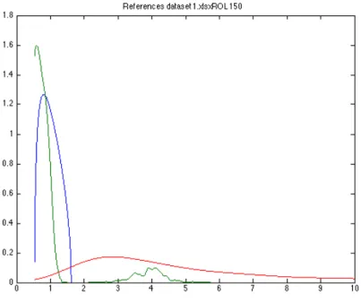
As an illustration, Figure 1 below contains the three reference distributions Θ1,

Θ_{2 and Θ3 for the number of assets contained inside Dataset 1 (eleven assets) and}

a rolling window of 150 days. We also included in appendix the three reference distributions computed for all the other datasets and the same rolling window of 150 days.

Figure 1: Reference distributions for Dataset 1. Blue: Marchenko Pastur (Θ1), Green: Θ2, Red: Θ3

3.2 Financial Crisis Indicators

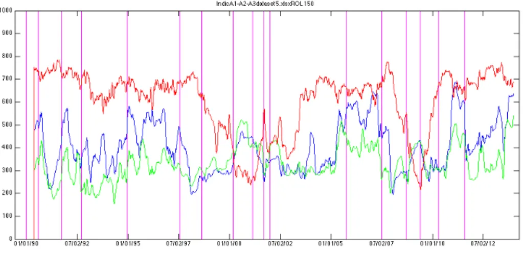
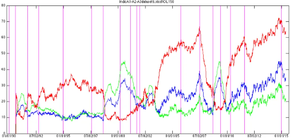
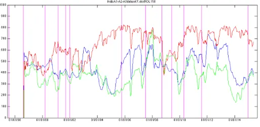
Using the tools described above, we build two kinds of ﬁnancial crisis indicators: the indicators of the A-series and the indicators of the B-series.

The indicators of the A-series compare at each date the empirical distribution of the spectrum of the covariance matrix to the references that we introduced in the previous subsection. We chose to use the Hellinger distance in its discrete form as introduced by Hellinger (1909). We decided to use this metric on the space of distribution instead of the Kullback–Leibler divergence introduced in Kullback and

(24)

Leibler (1951), which is also of very common use in probability theory, because we wanted a true metric, which the Kullback–Leibler divergence is not since it does not satisfy the triangle inequality. The Kullback–Leibler divergence is also not symmetric with respect to the two distributions considered. Moreover, since we chose an empirical approach with a strong focus on the intuitive aspect of the study, we felt that the Hellinger distance, which is plainly the Euclidean distance of the square root of the components, was easier to see when drawing two distribu-tions on the same graphic than the Kullback–Leibler divergence which is deﬁned as the expectation of the logarithmic diﬀerence between the two distributions.

We recall that the Hellinger distance D between two probability distributions

with densities P (x) and Q(x), which are both known at a number of points Xi,

(i œ J1, KK), is computed using the formula below :

D2 = K ÿ i=1 (ÒP (Xi) ≠ Ò Q(Xi))2 (9)

Considering any of the three reference distributions, we compute at each date its Hellinger distance to the empirical distribution of the eigenvalues of the covari-ance matrix. Our assumption is that the further away in the sense of the Hellinger distance the empirical distribution drifts away from the calm market reference, and the closer in the sense of the Hellinger distance the empirical distribution comes to the market in turmoil reference, then the more likely it becomes that the market is about to experience a crisis. Indeed, such movements tend to indicate a build-up of correlation and volatility inside the market. There is however no way to study those two eﬀects, volatility and correlation, separately in the Hellinger distance approach and the indicators of the A-series always lump those two instability fac-tors together in their forecasts of ﬁnancial crises.

Since all datasets except Dataset 6 only have a small number N of assets and will therefore give us only a small number of eigenvalues at each date, we combine at each date t the spectra obtained from the previous 20 days in order to have 20.N eigenvalues, which is enough observations, to derive a distribution by using a normalized histogram. We then compute the Hellinger distance to the reference distribution on a suﬃciently large support in order to capture all of the spectral distribution. In empirical studies such as Stanley and al. (2000), eigenvalues of the covariance matrix have been observed to grow as large as twenty ﬁve times

the critical value ⁄+ _{of Marchenko Pastur’s distribution (4). In consequence, we}

decided to consider 25 times the support [⁄≠

, ⁄+_{] in order to account for all of the}

(25)

The indicators of the ﬁrst type are the following. There are three of them, corresponding to the three reference distribution that we have introduced before:

• Indicator A1: It is the Hellinger distance between a modiﬁed version Eú

1(x),

detailed below, of the empirical distribution E (x) of the eigenvalues of the covariance matrix and the theoretical distribution of Marchenko Pastur Θ1. Indeed, Indicator A1, as well as all the indicators based on the Hellinger distance, needed to be adapted to filter out the effects of a parasitic phe-nomenon consisting of an accumulation of small eigenvalues close to zero, which deforms the unmodified empirical distribution and distorts the com-putation of its Hellinger distance with respect to the reference distribution. We illustrate this in Figure 2 and Figure 3:

Figure 2

Accumulation of Small Eigenvalues for Θ2

Figure 3

Accumulation of Small Eigenvalues for Θ3

In those two examples, which are very typical of the situations that we encounter in practice for a given date t while using all the datasets, we see the

(26)

reference distribution (in blue) and we see the empirical distribution of the eigenvalues of the covariance matrix (in green). The empirical distribution can differ from the reference distribution in two ways. It can overflow to the right toward the higher eigenvalues: that’s the kind of behavior that we are looking for in order to detect a financial crisis. It can also unfortunately accumulate itself, sometimes most of the mass is even there, closer to zero toward the very small eigenvalues. Such a behavior of the distribution of the eigenvalues of the covariance matrix is more indicative of the prevalence of risk free combinations of assets which equates to a very calm and diversified market.

The solution was to deﬁne A1 and the A-series indicators in the following way : instead of computing the Hellinger distance between the unmodiﬁed empirical distribution E and the Marchenko Pastur reference Θ1, we compute

the Hellinger distance between Θ1 and the distribution Eú

1 deﬁned in the following way : Eú 1(x) = min(E (x), Θ1(x)), x < ⁄+ 10 (10) Eú 1(x) = E (x), x > ⁄+ 10 (11) Therefore : A1 = D{Eú 1, Θ1} (12)

For a given dataset, this indicator measures at each date by how much the assumptions of Marchenko Pastur’s theorem (normal i.i.d coefficients of vari-ance equal to 1) are violated. Since the finite size of the rolling covarivari-ance matrix does not change over time, it will not be responsible for any dynam-ical variations of the Hellinger distance although it does certainly account for part of the distance between the theoretical asymptotic distribution of Marchenko Pastur and the empirical distribution. This indicator lumps to-gether the apparition of non-normality, correlations and volatility in the log-return time series, it cannot differentiate between all those effects but it is still very useful. As a matter of fact, the apparition of any of those phe-nomena, whose effects are not expected to compensate one another, can be interpreted as a warning that a crisis might be around the corner. Therefore our assumption is going to be that the further away the modified empirical

distribution Eú

(x) becomes from the reference Marchenko Pastur distribu-tion in the sense of the Hellinger distance, the more likely a crisis is going to happen in the near future.

(27)

Like we said earlier, using the Marchenko Pastur distribution for a given aspect ratio as a reference distribution might not be optimal because it is an asymptotic result and we deal with finite size matrices and because even a perfectly calm financial market might be better modeled by random matrices of coefficients with some natural correlations.

• Indicator A2: It is the Hellinger distance between the modiﬁed version Eú

2(x),

detailed below, of the empirical distribution of the eigenvalues of the covari-ance matrix E (x) and the simulated reference distribution Θ2. Since corre-lated Gaussian coeﬃcients are supposed to better model the market situa-tion, we expect Θ2 to provide a better calm market reference from which to measure a drift of the empirical distribution of the eigenvalues of the covari-ance matrix in the times leading up to a ﬁnancial crisis. Like with Indicator A1, we decided to work on 25 times the support of the corresponding theo-retical Marchenko Pastur distribution and the same issues of accumulation of the empirical distribution toward the small eigenvalues in time of mar-ket calm presented itself. There is no closed form formula for the reference

Θ_{2 and we cannot assume that its support is bounded like the support of}

Marchenko Pastur’s distribution is bounded by ⁄≠

and ⁄+ _{so we decided to}

keep ⁄ú ₌ ⁄+

10 as a threshold, such that an abundance of very small

eigenval-ues would not make the Hellinger distance explode. Therefore, we compute

the Hellinger distance between Θ2 and Eú _{in the following manner :}

Eú 2(x) = min(E (x), Θ2), x < ⁄ú (13) Eú 2(x) = E (x), x Ø ⁄ ú (14) Therefore : A2 = D{Eú 2, Θ2} (15)

• Indicator A3: It is the Hellinger distance between the modiﬁed version Eú

3(x),

detailed below, of the empirical distribution of the eigenvalues of the covari-ance matrix E (x) and the simulated reference distribution Θ3. We included very fat tails (coeﬃcients that follow a Student (t=3) distribution) as a way to model crisis conditions, therefore Indicator A3 is an inverted indicator. Indeed, it produces red ﬂags when it is getting small, which means that the empirical distribution of the eigenvalues of the covariance matrix is getting very close to Θ3, with is extremely heavy tailed and represents a spectrum entirely shifted toward the large eigenvalues, characterizing a market in deep turmoil. When the market goes from a calm state to a crisis state, the mod-eling that we make of the log-returns goes from a Gaussian to a Student

(28)

(t=3) distribution. As a remark, we did not include skewness in the random coeﬃcients from which we derive the reference distributions because ﬁnancial log-returns do not typically present persistent skewness, especially over the time periods considered for the rolling window, as demonstrated in the work of Singleton and Wingender (1986). We retain for A3 the same method of computation as in the other ones of the A-series. We compute it over 25 times the support of the corresponding theoretical Marchenko Pastur distribution

and the threshold ⁄ú ₌ ⁄+

10 is used to ﬁlter out the very small eigenvalues.

Indicator A3 then computes at each date t the Hellinger distance between

Θ_{3 and E}ú _{such that :}

Eú 3(x) = min(E (x), Θ3), x < ⁄ ú (16) Eú 3(x) = E (x), x Ø ⁄ ú (17) Therefore : A3 = D{Eú 3, Θ3} (18)

We therefore have three indicators of the first type, called A1, A2 and A3. Each possesses its own characteristics and looks at specific market conditions that may be indicative of an impending financial crisis. We do expect the three indicators of the first kind to be coherent with one another, especially since they are of similar origin, but they also complement one another and the financial crisis forecasts that we make need to take all three into consideration to be effective.

We now shift to the indicators of the B-series. At each date t, the centered

rolling matrix ROLú_{(t) in formula (1) contains two components: a volatility}

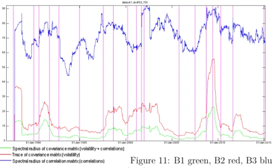
com-ponent and a correlation comcom-ponent. The indicators of the B-series are based on those two components. As we are going to see, both components are important, but the relative strength of their signal will greatly depend on the choice of the dataset we use. We build at each date t the three indicators of the second type in the following way :

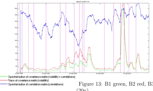
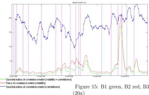
• Indicator B1: It is defined as the spectral radius of the covariance matrix CV (t) in formula (2). It measures a mixed signal depending on both volatil-ity and correlations in the market. A larger value for the spectral radius is indicative of dynamical instability and increased correlations in the system but it also takes the volatility effect into account since we are working with a covariance instead of a correlation matrix. This indicator takes the effects of both volatility and correlations into account and those two effects are not supposed to compensate each other, on the contrary they are expected to evolve in the same direction in the times leading up to a financial crisis as it was demonstrated by Sandoval Junior and De Paula Franca (2012).

(29)

• Indicator B2: It is defined as the trace of the covariance matrix CV (t). It measures the volatility signal alone. While it may seem at first that B2 lacks a very important aspect of what is happening inside the market, we will see while discussing experimental results that it is still a very good financial crisis indicator. It is also very easy and fast to compute. As a matter of fact it is not even needed to compute the whole spectrum of the covariance matrix to compute its trace.

• Indicator B3: It is deﬁned as the spectral radius of the correlation matrix CR(t) in formula (3). It measures the correlation signal alone. The useful-ness of Indicator B3 greatly depends on the choice of the dataset. We will discuss more about this in the section discussing the numerical results. Only when used on Dataset 6, which contains a large number of assets, which are individual stocks components of an index, does indicator B3 realize its full potential. Indeed, there is a lot averaging eﬀect inside an index and when we use the value of the index itself as opposed to its individual components, the correlation signal is generally smothered. The potential of Indicator B3 is great however, because unlike with the study of volatility alone, the study of correlation may be the only way to give the indicators that we have built real predictive power. Since Dataset 6 also features daily volume and daily market capitalization data, we also build the following variations of indicator B3, to be used on Dataset 6 exclusively:

– Indicator B3A: the spectral radius of the matrix CR1(t). Its coeﬃcients

are those of CR(t) which have been weighted at each date t by the market capitalization (cap(t)) expressed in dollars, in the following way

for a dataset containing F assets. ’(i, j) œ [1, F ]2 _:

CR1(t)(i, j) = CR(t)(i, j).

cap(t)(i).cap(t)(j)

qF

k=1cap(t)(k)2

(19)

– Indicator B3B: the spectral radius of the matrix CR2(t). Its coeﬃcients

are those of CR(t) which have been weighted at each date t by the vol-ume of stocks exchanged (volu(t)) expressed in dollars, in the following

way for a dataset containing F assets. ’(i, j) œ [1, F ]2 _:

CR1(t)(i, j) = CR(t)(i, j).

volu(t)(i).volu(t)(j)

qF

k=1volu(t)(k)2

(20)

– Indicator B3C: Since indicator B3B will prove useful but will also usu-ally produce a noisy signal, B3C is computed at each date t as a moving

Financial crisis forecasts and applications to systematic trading strategies

HAL Id: tel-01927767

https://tel.archives-ouvertes.fr/tel-01927767

Financial crisis forecasts and applications to systematic

trading strategies

Antoine Kornprobst

To cite this version:

UNIVERSIT´

E PARIS I PANTH´

EON-SORBONNE

´

ECOLE DOCTORALE ED-465

CENTRE D’´

ECONOMIE DE LA SORBONNE

Th`

ese

DOCTEUR DE L’UNIVERSIT´

E PARIS I

PANTH´

EON-SORBONNE

Antoine Kornprobst

Financial Crisis Forecasts and Applications

to Systematic Trading Strategies

Acknowledgements

Introduction

Chapter 1

�������������������������

����������������������������

�������������������������

An Empirical Approach to Financial Crisis

Indicators Based on Random Matrices

Raphael Douady

and Antoine Kornprobst

Stony Brook University, Université Paris 1 Panthéon-Sorbonne

Université Paris 1 Panthéon Sorbonne, Labex ReFi

September 5th 2017

1

Introduction

2

The Data

3

Methodology

3.1

Framework

3.2

Financial Crisis Indicators

��

��

��

_{Stony Brook University, Université Paris 1 Panthéon-Sorbonne}

_{Université Paris 1 Panthéon Sorbonne, Labex ReFi}