Evolution of stratospheric ozone in the mid-latitudes in connection with the abundances of halogen compounds

(1)

HAL Id: tel-00733555

https://tel.archives-ouvertes.fr/tel-00733555

Submitted on 18 Sep 2012

HAL is a multi-disciplinary open access

archive for the deposit and dissemination of

sci-entific research documents, whether they are

pub-lished or not. The documents may come from

teaching and research institutions in France or

abroad, or from public or private research centers.

L’archive ouverte pluridisciplinaire HAL, est

destinée au dépôt et à la diffusion de documents

scientifiques de niveau recherche, publiés ou non,

émanant des établissements d’enseignement et de

recherche français ou étrangers, des laboratoires

publics ou privés.

Evolution of stratospheric ozone in the mid-latitudes in

connection with the abundances of halogen compounds

Prijitha Gopalapillai

To cite this version:

Prijitha Gopalapillai. Evolution of stratospheric ozone in the mid-latitudes in connection with the

abundances of halogen compounds. Atmospheric and Oceanic Physics [physics.ao-ph]. Université

Pierre et Marie Curie - Paris VI, 2012. English. �tel-00733555�

(2)

UNIVERSITY OF PIERRE AND MARIE CURIE - PARIS VI

Doctoral school of the Environmental Sciences / ED129

P H D T H E S I S

prepared at the laboratory CNRS/LATMOS to obtain the degree of

Doctor of Philosophy

(Specialisation : Physics)

publicly presented and defended by

GOPALAPILLAI Prijitha (Prijitha J. Nair)

on 09 March 2012

Evolution of stratospheric ozone in the mid-latitudes in

connection with the abundances of halogen compounds

The Jury

Dr. Nathalie Huret LPCE/CNRS, Orléans, France Referee

Dr. Philippe Ricaud Météo-France/CNRS, Toulouse, France Referee

Pr. François Ravetta LATMOS/CNRS, Paris, France President

Dr. Philippe Keckhut LATMOS/CNRS, Guyancourt, France Invited Examiner

Dr. Chantal Claud LMD/CNRS, Palaiseau, France Examiner

Dr. Corinne Vigouroux IASB - BIRA, Brussels, Belgium Examiner

(3)

(4)

3 Stability of ozone measurements at OHP 39 3.1 Ozone Measurements . . . 40 3.1.1 Umkehr . . . 40 3.1.2 Ozonesondes . . . 40 3.1.3 SBUV(/2). . . 41 3.1.4 SAGE II. . . 42 3.1.5 HALOE . . . 42 3.1.6 GOMOS. . . 42 3.1.7 MLS . . . 43 3.2 Methodology . . . 43 3.2.1 Data screening . . . 43 3.2.2 Coincidence criteria . . . 44 3.2.3 Data conversion . . . 45 3.2.4 Data analysis . . . 47

3.3 Vertical distribution of mean bias . . . 49

3.3.1 Long-term data sets . . . 50

3.3.2 Short-term data sets . . . 52

3.4 Temporal evolution . . . 52

3.4.1 Comparison of Umkehr with lidar . . . 52

3.4.2 Comparison of ozonesondes with lidar . . . 54

3.4.3 Comparison of SAGE II and HALOE with lidar . . . 55

3.4.4 Comparison of SBUV(/2) with lidar . . . 56

3.4.5 Comparison of MLS and GOMOS with lidar . . . 57

3.5 Drift in ozone diﬀerences. . . 58

3.5.1 Sensitivity of standard deviations . . . 59

3.5.2 Signiﬁcance of the drifts in terms of the chosen standard deviation . 59 3.6 Summary . . . 63

4 Stability of ozone observations over NDACC lidar stations 65 4.1 Ozonesonde measurements . . . 66

4.2 Data analysis . . . 67

4.2.1 Relative diﬀerence and mean bias. . . 69

4.2.2 Data conversion . . . 69

4.3 Average biases: comparison with lidar measurements . . . 70

4.3.1 Correction factor . . . 73

4.4 Relative drifts. . . 74

4.4.1 Comparison with ozone lidar as reference . . . 74

4.4.2 Comparison of lidar with SBUV(/2), SAGE II and HALOE as references 75 4.4.3 Comparison of SBUV(/2), SAGE II and HALOE . . . 75

4.4.4 Average of the drifts of long-term measurements . . . 77

4.5 Combined data: SAGE II, HALOE and Aura MLS . . . 79

4.5.1 Time series . . . 79

4.5.2 Relative drifts of the combined time series . . . 82

(6)

Contents iii

5 Stratospheric ozone evolution in the northern mid-latitudes 85

5.1 Explanatory variables . . . 86

5.1.1 Quasi Biennial Oscillation . . . 87

5.1.2 Solar ﬂux . . . 87

5.1.3 Aerosols . . . 89

5.1.4 Eddy heat ﬂux . . . 89

5.1.5 North Atlantic Oscillation . . . 90

5.1.6 PWLT and EESC : Ozone trend estimation methods . . . 90

5.2 Multiple regression model and method . . . 92

5.3 Ozone total column measurements . . . 94

5.3.1 Evolution of ozone total column . . . 95

5.3.2 Ozone anomaly . . . 95

5.3.3 Comparison between Dobson and SAOZ at OHP: bias and drift. . . 96

5.4 Multiple regression analysis of ozone total column at OHP. . . 96

5.4.1 Contribution of proxies to ozone variability . . . 100

5.4.2 Trends in ozone total column . . . 102

5.5 Multiple regression analysis of ozone total column at MOHp. . . 103

5.5.1 Contribution of proxies to ozone variability . . . 106

5.5.2 Trends in ozone total column . . . 106

5.6 Vertically resolved ozone observations at OHP. . . 108

5.6.1 Stratospheric ozone evolution . . . 108

5.6.2 Stratospheric ozone anomaly . . . 109

5.6.3 Application of multiple regression. . . 109

5.6.4 Contribution of proxies to the variability of ozone proﬁles . . . 115

5.6.5 Trends in stratospheric ozone vertical proﬁles . . . 117

5.7 Connection between ozone proﬁle and column measurements . . . 118

5.8 Summary . . . 120

6 Summary, conclusions and perspectives 123 6.1 Summary and conclusions . . . 123

6.2 Perspectives . . . 125

(7)

(8)

Contents v

Acknowledgements

I would like to express my sincere gratitude to Dr. Sophie Godin-Beekmann for providing an opportunity and making available adequate funding to carry out my thesis under her supervision. She was inspiring and the routine discussions with her were thought-provoking. I appreciate her immense patience that helped me to develop a keen interest in the topic. Her generosity in giving full freedom to write articles is to be remembered. I also acknowledge her for spending her valuable time on critical reviews of my articles and comments on the thesis manuscript.

I am deeply conscious of my indebtedness to Dr. Jayanarayanan Kuttippurath (LATMOS), whose scientific guidance and moral support were crucial for developing my dissertation, scholarly writing and thinking skills and collegiate attitude. I greatly appreciate his comments on my manuscript and the scientific discussions with him. I also thank him for helping the extraction of Aura MLS data and his assistance in making the multiple regression model and heat flux data for the trend studies.

I wish to thank Dr. Philippe Keckhut (LATMOS) and Dr. Chantal Claud (LMD) for being a part of my thesis committee. I greatly appreciate the fruitful discussions I had with them during the course of my thesis and their comments on the thesis manuscript. Their encouragements will always be remembered.

I owe sincere thanks to Dr. Nathalie Huret (LPCE, Orléans) and Dr. Philippe Ricaud (Météo-France, Toulouse) for their critical review of my thesis and their encouraging thesis evaluation reports. Also, I thank Dr. Corinne Vigouroux (BIRA, Belgium) for her presence and comments during my thesis defence. I would like to convey my acknowledgment to Prof. François Ravetta (LATMOS) for being the President of the jury of my thesis defence committee.

This thesis makes use of ozone measurements from a number of instruments. The principal investigators of all those were very kind in providing relevant information to analyse the data. I wish to thank Dr. Florence Goutail (LATMOS), Dr. Gérard Ancellet (LATMOS), Dr. Andrea Pazmiño (LATMOS), Dr. Lucien Froidevaux (JPL, USA), Dr. Larry Flynn (NOAA, USA), Dr. Irina Petropavlovskikh (CIRES, USA), Dr. Wolfgang Steinbrecht (DWD, Germany), Dr. Hans Claude (DWD, Germany), Dr. Anne van Gijsel (RNMI, The Netherlands), Dr. Thierry Leblanc (JPL, USA), Dr. Jean-Christopher Lambert (BIRA, Belgium), Dr. Daan Hubert (BIRA, Belgium), Dr. Tetsuro Uekubo (JMA, Japan), Dr. Toshifumi Fujimoto (JMA, Japan) and Dr. Alan Thomas (NIWA, New Zealand).

I thank Dr. Danièle Hauser and Dr. Alain Hauchecorne, the directors of CNRS/LATMOS, for their hearty welcome to the laboratory to pursue my Ph.D. I also express my gratitude to Mrs. Laurence Touchon, the secretary of my Doctoral School, for helping me in all administrative matters related to the Doctoral School.

I would like to thank Mrs. Cathy Boonne (IPSL) for her timely help with the data and for maintaining ETHER data cluster. I thank Mr. Philippe Weill, the system administrator of the LATMOS, for all his assistance with my computers. I also remember Mrs. Michèle Moreau, Mrs. Maryse Grenier, Mrs. Evelyne Quinsac and Mrs. Valérie Fleury, the former and current secretaries of LATMOS for their help with the administrative formalities. I wish to thank Dr. Slimane Bekki (group head) and Dr. Marion Marchand (LATMOS) for their unconditional support and encouragement during the diﬃcult phase of my thesis tenure.

I take this opportunity to express my sincere gratitude to those who pray for my well-being. I must single out the help, encouragement, and moral support I received from the parents of my husband (Mr. K. R. S. Nair and Mrs. M. Balamani Amma), my parents (Late Mr. K. S. Gopala Pillai and Mrs. P. Renukadevi Amma), brother (Mr. Praveen G.), sister (Mrs. Preethisree G.), brother-in-law (Mr. Arun Kumar S. Nair), and sister-in-law (Mrs. Priya A. Nair). With great respect and aﬀection, I remember the eﬀorts of my beloved, who brought me to this position. Besides this, several people have knowingly and unknowingly helped me in the successful completion of this study. Finally, I really thank the extreme power that activates my life and controls my existence.

This thesis was supported by a funding from the GEOMON (Global Earth Observation and Monitoring of the atmosphere) European project.

(9)

(10)

Contents vii

Acronym

ACE-FTS : Atmospheric Chemistry Experiment-Fourier Transform Spectrometer

AER : Aerosol

AK : Averaging Kernel AO : Arctic Oscillation

BP : Bass and Paur

BD : Brewer-Dobson

BDM : Brion-Daumont-Malicet

Br : Bromine

CCM : Chemistry Climate Model

CCMVal : Chemistry Climate Model Validation CF : Correction Factor

CFC : Chloroﬂuorocarbon

CH4 : Methane

Cl : Chlorine

ClO : Chlorine monoxide

CIRA : COSPAR International Reference Atmosphere CO2 : Carbon dioxide

CTM : Chemical Transport Model DIAL : Diﬀerential Absorption Lidar

DOAS : Diﬀerential Optical Absorption Spectroscopy

DU : Dobson Unit

ECC : Electrochemical Concentration Cell

EESC : Equivalent Eﬀective Stratospheric Chlorine ENSCI : Environmental Science Corporation ENVISAT : Environmental Satellite

EP ﬂux : Eliassen-Palm ﬂux

ERBS : Earth Radiation Budget Satellite FTIR : Fourier Transform Infrared

GHG : Greenhouse gas

GOME : Global Ozone Monitoring Experiment

GOMOS : Global Ozone Monitoring by Occultation of Stars

H : Hydrogen

HALOE : Halogen occultation Experiment

HFX : Eddy heat ﬂux

HIRDLS : High Resolution Dynamics Limb Sounder HNO3 : Nitric Acid

H2O : water vapour

H2SO4 : Sulfuric Acid

IASI : Infrared Atmospheric Sounding Interferometer

IR : InfraRed

LIDAR : Light Detection And Ranging MetOp : Meteorological Operational MLS : Microwave Limb Sounder MLO : Mauna Loa Observatory

MOHp : Meteorological Observatory Hohenpeissenberg MSU : Microwave Sounding Unit

NAO : Northern Atlantic Oscillation

(11)

viii Contents

NAT : Nitric Acid Trihydrate

NCEP : National Center for Environmental Prediction NDACC : Network for the Detection of Stratospheric Change

NH : Northern Hemisphere

NO : Nitrogen Oxide

NO2 : Nitrous Oxide

NOAA : National Oceanic and Atmospheric Administration

O : Oxygen

ODS : Ozone Depleting Substance

OH : Hydroxyl

OHP : Haute-Provence Observatory OMI : Ozone Monitoring Instrument

OSIRIS : Optical Spectrograph InfraRed Imager System ppb : Parts per billion

ppm : Parts per million

ppt : Parts per trillion

PSC : Polar Stratospheric Cloud

PW : Piecewise

PWLT : Piecewise linear trend QBO : Quasi Biennial Oscillation

REPROBUS : Reactive processes ruling the ozone budget in the stratosphere SAGE : Stratospheric Aerosol and Gas Experiment

SAOZ : Système d’Analyse par Observation Zénithale SBUV : Solar Backscatter UltraViolet

SCIAMACHY : SCanning Imaging Absorption spectroMeter for Atmospheric CHartographY

SFX : Solar ﬂux

SFX : Solar ﬂux unit

SMR : Sub-millimetre Radiometer

SO2 : Sulfur Dioxide

SH : Southern Hemisphere

SPARC : Stratospheric Processes And their Role in Climate STS : Supercooled Ternary Solutions

SPC : Science Pump Corporation TMF : Table Mountain Facility

TOMS : Total Ozone Mapping Spectrometer UARS : Upper Atmosphere Research Satellite

UV : Ultraviolet

VMR : Volume Mixing Ratio

VP SC : Volume of PSC

(12)

Contents ix

PUBLICATIONS Peer-Reviewed

(1) Nair, P. J., Godin-Beekmann, S., Pazmiño, A., Hauchecorne, A., Ancellet, G., Petropavlovskikh, I., Flynn, L. E., and Froidevaux, L.: Coherence of long-term stratospheric ozone vertical distribution time series used for the study of ozone recovery at a northern mid-latitude station, Atmos. Chem. Phys., 11, 4957–4975, doi:10.5194/acp-11-4957-2011, 2011.

(2) Nair, P. J., Godin-Beekmann, S., Froidevaux, L., Flynn, L. E., Zawodny, J. M., Russell III, J. M., Pazmiño, A., Ancellet, G., Steinbrecht, W., Claude, H., Leblanc, T., McDermid, S., van Gijsel, J. A. E., Johnson, B., Thomas, A., Hubert, D., Lambert, J.-C., Nakane, H., and D. P. J. Swart: Relative drifts and stability of satellite and ground-based stratospheric ozone proﬁles at NDACC lidar stations, Atmos. Meas. Tech., 5, 1301–1318, doi:10.5194/amt-5-1301-2012, 2012.

(3) Godin-Beekmann, S., and Nair, P. J.: Sensitivity of stratospheric ozone lidar measurements to a change in ozone absorption cross-sections, J. Quant Spectrosc Radiat Transfer, doi:10.1016/j.jqsrt.2012.03.002, 2012.

In preparation

(4) Nair, P. J. et al.: Trends and variability in the vertical distribution of stratospheric ozone at Observatoire de Haute-Provence (OHP).

(5) Griesfeller A., Godin-Beekmann S., Petropavlovskikh, I., Nair, P. J., Griesfeller J., Evans, R. D., and Pazmiño, A.: Comparison of long-term stratospheric ozone time series from lidar and Umkehr measurements at Observatoire de Haute-Provence (OHP), 44◦_{N, 6}◦_E.

Conference Abstracts

(6) Nair, P. J., Godin-Beekmann, S., Froidevaux, L., Flynn, L. E., Ancellet, G., Steinbrecht, W., Claude, H., Nakane, H., Leblanc, T., McDermid, S., Swart, D. P. J., van Gijsel, J. A. E., and Thomas, A.: Relative drifts of stratospheric ozone measurements at NDACC lidar stations, Geophysical Research Abstracts, European Geosciences Union (EGU) General Assembly, 13, EGU2011-10825, 2011.

(7) Nair, P. J., Godin-Beekmann, S. and Pazmiño, A.: Coherence of long-term strato-spheric ozone time series for the study of ozone recovery in the northern mid-latitudes, Geophysical Research Abstracts, European Geosciences Union (EGU) General Assembly, 12, EGU2010-5519, 2010.

(8) Godin-Beekmann, S., Nair, P. J., Froidevaux, L., Flynn, L. E., Ancellet, G., Steinbrecht, W., Claude, H., Nakane, H., Leblanc, T., McDermid, S., Swart, D. P. J., van Gijsel, J. A. E., and Thomas, A.: Relative drifts of stratospheric ozone measurements at NDACC lidar stations, NDACC symposium, 7–10 November 2011.

(13)

x Contents

(9) Godin-Beekmann, S. and Nair, P. J.: Short term and long-term evolution of strato-spheric ozone at a northern mid-latitude station, NDACC symposium, 7–10 November 2011. (10) Griesfeller, A., Godin-Beekmann, S., Nair, P. J., Goutail, F., Hendrick, F., Ionov, D., Pazmiño, A., Petropavlovskikh, I., Pommereau, J.-P., van Roozendael, M.: Long-term time series of ozone at Observatoire de Haute-provence (OHP), 44◦_{N, 6}◦_E,

Geophysical Research Abstracts, European Geosciences Union (EGU) General Assembly, 11, EGU2009-9262, 2009.

Reports

(11) Scientiﬁc Assessment of Ozone Depletion 2010: Stratospheric Ozone and Surface Ultraviolet Radiation edited by Anne Douglass and Vitali Fioletov. (Contributed)

(12) Godin-Beekmann, S., Nair, P. J., NDACC lidar and satellite measurement teams: What NDACC ozone lidars are telling us about long-term satellite measurements, ISPARC/IO3C/WMO-IGACO Workshop on Past changes in the Vertical Distribution of Ozone, Geneva, 25–27 January 2011.

(13) Godin-Beekmann, S. and Nair, P. J.: The eﬀect of change of BP to DBM ozone absorption cross-sections on lidar measurements, IO3C-WMO-IGACO-O3/UV, Meeting on ozone absorption cross-section, Geneva, 23–25 March 2010.

(14) Godin-Beekmann, S., and Nair, P. J.: Sensitivity of stratospheric ozone lidar measurements on ozone cross-section, http://igaco-o3.fmi.ﬁ/ACSO, 2010.

(14)

Contents xi

Abstract

This thesis addresses the issue of the long-term evolution of stratospheric ozone in relation to the halogen loading. To that aim, long-term records of satellite and ground-based (GB) ozone profile measurements at six lidar stations, of the Network for the Detection of Stratospheric Change, are examined to find the bias and drift in the measurements. The stratospheric ozone trends are then estimated from the ozone profile and total column measurements using the Equivalent Effective Stratospheric Chlorine time series and two linear trend functions (before and after 1997) called as piecewise linear trends (PWLTs), to account for the change in the trends of ozone depleting substances, at Northern mid-latitude stations. The analysis uses GB measurements from lidar, Umkehr, ozonesondes and the Dobson and SAOZ spectrometers, and satellite observations from SBUV(/2), SAGE II, HALOE, UARS MLS, Aura MLS and GOMOS. First of all, a sensitivity analysis is performed to diagnose the effect of using different ozone absorption cross-section data sets (Bass and Paur and Brion-Daumont-Malicet) on the retrieved lidar ozone profiles. The relative ozone differences computed using those two cross-section data are less than ±1% from 10 to 35 km at all latitudes, except a −1.5% deviation at 15 km in the tropics. Above 35 km, the deviations increase with a maximum of 1.7% in the tropics and a minimum of 1.4% in the high latitudes. The stability of various GB and satellite ozone profile time series is then evaluated by comparing with the ozone lidar data for each station. All ozone profile measurement techniques show their best agreement (±3%) with lidars in the 20–40 km altitude range and the estimated drifts are less than ±0.3%yr−1 _{at all stations.}

Comparatively large biases and drifts are computed below 20 and above 40 km. A combined time series of the relative diﬀerences of SAGE II, HALOE and Aura MLS with respect to the lidar measurements at the six lidar sites is constructed to obtain long-term data sets from 1985 to 2010. The relative drifts derived from these combined data of ∼27 years are very small, within ±0.2%yr−1_{. Then, stratospheric ozone trends are estimated at Meteorological}

Observatory Hohenpeissenberg (MOHp) using Dobson, and at Haute-Provence Observatory (OHP) using Dobson and SAOZ total column measurements and various GB and satellite ozone profiles. For that a multiple regression model is developed using different explanatory variables such as Quasi Biennial Oscillation (QBO), North Atlantic Oscillation (NAO), solar flux, eddy heat flux, aerosols and trend. The PWLTs computed from the ozone column at OHP and MOHp show significant negative (−1.4 ± 0.29 DU yr−1_{) and positive}

(0.55 ± 0.29 DU yr−1_{) values before and after 1997, respectively, indicating a clear signal}

of ozone recovery at these latitudes after 1996. Vertical distribution of ozone trends based on PWLT model, estimated using the all instrument average at OHP exhibit about −0.5 ± 0.1 % yr−1 _{in the 16–22 km range and about −0.8 ± 0.2 % yr}−1 _{in the 38–45 km region}

before 1997. Signiﬁcant positive trends (0.2 ± 0.05–0.3 ± 0.1 % yr−1_{) are estimated in the}

15–45 km altitude region after 1996. These significant ozone profile trends in the respective periods corroborate those derived from the ozone total column and hence, provide signs of ozone recovery in the northern mid-latitudes. The trends based on both PW and EESC regressions are similar and significant before 1997 while they differ slightly after 1996, with the largest value in the PW regression. In addition, the most recent increase in ozone after 1996 is due to the increase in QBO and planetary wave drive. For instance, QBO, NAO and heat flux contribute about 20–26 DU to the large total ozone anomaly of 25–30 DU in the winter/spring months in 2010. Therefore, this thesis presents some new and interesting results on the mid-latitude stratospheric ozone recovery.

(15)

(16)

Contents xiii

Résumé

Cette thèse a pour objet l’étude de l’évolution à long terme de l’ozone stratosphérique, en liaison avec la variation dde l’abondance des composés halogénés dans la moyenne at-mosphère. Dans ce but, les longues séries de mesures sol et satellitaires de la distribu-tion verticale d’ozone obtenues depuis les années 1980 sont évaluées dans six stadistribu-tions du Network for the Detection of Atmospheric Composition Changes (NDACC - réseau inter-national de surveillance de la composition atmosphérique), pour déterminer les biais et dérives éventuelles entre les mesures. Les tendances d’ozone stratosphérique sont ensuite évaluées dans deux stations de moyenne latitude de l’hémisphère nord à l’aide d’un modèle statistique utilisant deux types d’indicateurs pour représenter l’évolution des substances destructrices d’ozone dans la stratosphère: (1) l’Equivalent Effective Stratospheric Chlo-rine (EESC - paramètre quantifiant l’effet des composés chlorés et bromés stratosphériques sur l’ozone) et (2) deux fonctions linéaires avec changement de pente en 1997. L’étude de tendance est effectuée pour les mesures du contenu intégré d’ozone dans les deux sta-tions et les mesures de distribution verticale à l’Observatoire de Haute-Provence. L’étude utilise les mesures sol d’ozone obtenues par lidar (profil d’ozone), spectromètre Dobson (contenu intégré et profil d’ozone par la méthode Umkehr), ozonosondage (profil d’ozone) et spectromètre UV-Visible SAOZ (contenu intégré). Les observations satellitaires utilisées proviennent des instruments SBUV(/2), SAGE II, HALOE, UARS MLS, Aura MLS et GOMOS. Tout d’abord une étude de la sensibilité des mesures lidar aux sections efficaces d’ozone utilisées dans l’algorithme de restitution est effectuée. La différence relative d’ozone obtenue à partir des mesures restituées à l’aide de différents jeux de données de section ef-ficace reconnues par les instances internationales, est inférieure à ±1% entre 10 et 35 km à toutes les latitudes (à l’exception de -1.5 % à 15 km aux tropiques). Au-dessus de 35 km, l’écart s’accroit, avec un maximum à 45 km de 1.7 % aux tropiques et un minimum de 1.4 % aux hautes latitudes. La stabilité des différentes séries de mesures satellitaires et sol de la distribution verticale d’ozone est ensuite évaluée à partir de la comparaison avec les mesures lidar dans les six stations NDACC considérées au cours de la thèse. Le meilleur accord (±3%) entre les mesures issues des différentes techniques et les mesures lidar est obtenu entre 20 et 40 km. Dans ce domaine d’altitude, la dérive entre les dif-férentes mesures est inférieure à ±0.3%yr−1_{. Des dérives et des biais comparativement}

plus importants sont calculés en dessous de 20 km et au-dessus de 40 km. Par ailleurs, la stabilité à plus long terme des mesures d’ozone est étudiée à partir de séries temporelles combinant les différences relatives entre les mesures lidar et les mesures SAGE II et HALOE d’une part avec les différences relatives entre les mesures lidar et les les mesures Aura MLS d’autre part. Les dérives estimées à partir de ces séries composites couvrant 27 années de mesure sont très faibles, de l’ordre de ±0.2%yr−1_{. Enfin les tendances évolutives du}

con-tenu intégré d’ozone sont évaluées à l’Observatoire Météorologique de Hohenpeissenberg (MOHp - Allemagne) à partir des mesures du spectromètre Dobson et à l’Observatoire de Haute-Provence (OHP - France) à partir des mesures des spectromètres Dobson et SAOZ. A l’OHP, les tendances de la distribution verticale d’ozone sont calculées à partir des mesures obtenues par différentes techniques de mesures, sol et satellitaires. Pour ce faire, un mod-èle de régression multilinéaire est développé, fondé sur l’utilisation de différentes variables telles que l’oscillation quasi-biennale (QBO), l’oscillation Nord-Atlantique (NAO), le flux solaire, le flux de chaleur turbulent, l’épaisseur optique des aérosols stratosphériques et les tendances à long terme. L’estimation des tendances calculées à partir des mesures de con-tenu intégré d’ozone dans les deux stations fournit des valeurs significatives, de l’ordre de −1.4 ± 0.29 DUyr−1_{) et 0.55 ± 0.29 DUyr}−1_{respectivement avant et après 1997. Les valeurs}

(17)

xiv Contents

positives de la tendance après 1997, significatives pour un intervalle de confiance de 95 %, montrent clairement un début de rétablissement de l’ozone stratosphérique à ces latitudes. Concernant la distribution verticale d’ozone, les tendances calculées à partir de la moyenne des différentes séries de données à l’OHP montrent des valeurs maximales en valeur absolue de l’ordre de −0.5 ± 0.1 %yr−1 _{entre 16 et 22 km et de −0.8 ± 0.2 %yr}−1_{entre 38 et 45 km}

avant 1997. Des tendances positives signiﬁcatives (0.2 ± 0.05–0.3 ± 0.1 %yr−1_{) sont évaluées}

entre 15 et 45 km après 1996. Ces tendances significatives du profil vertical d’ozone avant et après 1997 corroborent les résultats obtenus à partir du contenu intégré d’ozone et con-firment le début de rétablissement de l’ozone stratosphérique. Par ailleurs, dans les deux cas (contenu intégré d’ozone et distribution verticale), les tendances post-1997 restituées par le modèle utilisant les fonctions linéaires sont plus élevées que celles issues du modèle utilisant l’EESC, indiquant ainsi que d’autres paramètres contribuent à l’augmentation du contenu en ozone. Enfin, il a été constaté que les contenus intégrés élevés d’ozone observés ces dernières années étaient liés à l’influence de la QBO et des processus dynamiques. Ainsi la QBO, la NAO et le flux de chaleur turbulent expliquent environ 80 % de l’importante anomalie positive de 25 - 30 DU mesurée entre février et avril 2010.

(18)

Contents xv

Preface

Since the discovery of the Antarctic ozone hole in 1985 (Farman et al., 1985), several additional ground-based (GB) and satellite sensors have been employed globally for intense and constant monitoring of stratospheric ozone in the framework of World Meteorological Organisation - Global Atmosphere Watch (WMO–GAW) programme. The identiﬁcation of the role of chloroﬂuorocarbons in ozone loss process leads to drafting the Montreal Protocol and related amendments for limiting the production of such ozone depleting substances (ODSs) (WMO,1992). It resulted in the reduction of atmospheric concentration of ODSs (Mäder et al., 2010) and (Jones et al., 2011). Recently, ODSs has decreased to such an extent that the ozone shows stabilisation from 1997 onwards in the lower (WMO, 2011) and upper stratosphere (Steinbrecht et al.,2006) of the mid-latitudes.

Since, several factors affect the long-term evolution of ozone, it is important to assess the real reason for changes in ozone to identify the effects of reduction in ODSs on ozone and thus, to assess the effectiveness of the Montreal Protocol. To address this issue, highly stable ozone measurements spanning over several decades are necessary. Satellite measurements are usually prone to degradation at the end of their life span (WMO,2007). All long-term satellites that started in late 1970s and early 1990s (SAGE and HALOE) have stopped measurements in the mid-2000s. Even though new satellites have been launched since the early 2000s (ODIN, ENVISAT, Aura and MetOp), their observation records are too short to be used for ozone trend studies. In addition, some measurements are yet to be thoroughly validated for such kind of analysis.

The Network for the Detection of Atmospheric Composition Change (NDACC), another international network, which relies on worldwide measurements from GB stations using various instruments was established in 1991. It was designed initially for the simultaneous monitoring of various atmospheric parameters that play a key role in the stratospheric ozone depletion, with the primary aim of validating satellite measurements. Since any signiﬁcant drift in the data produces inaccurate trends, a careful evaluation of these data is inevitable. As the main goal of this thesis is the assessment of ozone trends, a stability analysis of the ozone measurements is necessary. Therefore, we ﬁrst analyse the stability various GB (lidars, ozonesondes, Umkehr, Dobson and SAOZ) and space-based (SBUV(/2), SAGE II, HALOE, UARS MLS, Aura MLS and GOMOS) measurements at the NDACC lidar sites. Then, these measurements are used for the estimation of stratospheric ozone trends.

Chapter 1 presents an overview of the general features of stratospheric chemistry and dynamics to follow the discussions presented in this thesis. The formation, transport, destruction and recovery of ozone in the stratosphere are reviewed in this chapter.

Since ozone lidar measurements are integral part of this study, a detailed description of lidar characteristics, data retrieval of ozone lidar and the general features of different lidars are given in Chapter2. Moreover, a sensitivity test is performed to find out the differences in retrieving ozone number density when using different ozone absorption cross-sections and meteorological data, with the aim of improving ozone lidar algorithm.

The next step is to assess the quality of these ozone lidar measurements for validating other GB and satellite data sets. To this end, we have performed the comparison of all available GB and satellite data at OHP. A thorough statistical analysis is carried out to ﬁnd any bias or drift in the ozone measurements of the GB and satellite data records at this mid-latitude station and the results are presented in Chapter3.

This analysis is further extended to all mid-latitude and subtropical lidar stations in Chapter4. Several statistical analyses are carried out for the accurate evaluation of relative drifts. This chapter also assesses the possibility of extending the terminated satellite data

(19)

xvi Contents

with the new satellite measurements (for e.g., SAGE II/HALOE and Aura MLS) to obtain a long-term data set spanning over several decades for ozone trend studies.

Since the ultimate goal of this thesis is to diagnose the trends in stratospheric ozone, these well validated and bias corrected data sets from GB and satellite instruments are used for the computation of ozone trends and the results are given in Chapter 5. A regression model using various explanatory variables is developed for this purpose and is applied to the GB and satellite data for the discussion of the derived trends. Further, response of ozone at diﬀerent latitudes and seasons with respect to several explanatory variables are also investigated here.

(20)

List of Figures

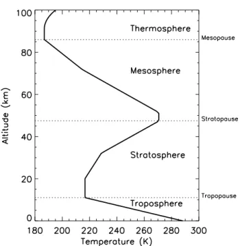
1.1 Schematic representation of the thermal structure of the atmospheric tem-perature based on the US Standard Atmosphere (1976). . . 2

1.2 Vertical distribution of the relative contribution of various reaction cycles in depleting ozone at various latitudes (fromBrasseur et al.,1999). . . 5

1.3 Monthly mean ozone total column abundance in DU from the TOMS ob-servations averaged in 1979–1986 as function of latitude and season (from

Brasseur et al., 1999). . . 6

1.4 Schematic representation of the stratospheric circulation (fromHolton et al.,

1995). . . 7

1.5 An illustration of the Antarctic ozone hole in 2006 (source : NASA). . . 8

1.6 Schematic diagram showing various chemical and dynamical processes in-volved in the destruction of ozone in the Antarctic polar vortex (source :

Brasseur et al., 1999). . . 9

1.7 Schematic view of PSC in the Antarctic stratosphere (source : NASA).. . . 10

1.8 Total ozone average in March and October in the northern and southern hemispheres, respectively. The horizontal Gray lines are the average total ozone prior to 1983 in March (NH) and October (SH) and the symbols rep-resent the satellite data in diﬀerent years. . . 11

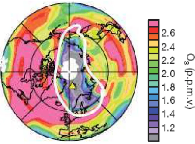
1.9 Arctic ozone loss in mid-March 2011 at an altitude of ∼20 km (Taken from

Manney et al.,2011).. . . 12

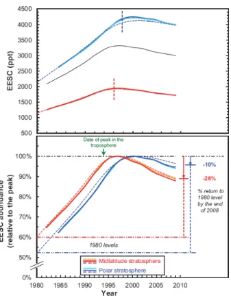
1.10 A diagram showing the evolution of stratospheric EESC in ppt (top panel) and in % (bottom panel) in the mid-latitude and polar stratosphere. . . 14

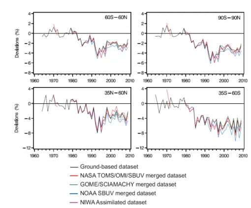
1.11 The deseasonalised total ozone deviations in 1964–2009 for the latitude bands (60◦_S–60◦_{N, 90}◦_S–90◦_{N, 35}◦_N–60◦_{N and 35}◦_S–60◦_{S) estimated from}

diﬀer-ent data sets. The zero line indicates the pre-1980 level (Taken fromWMO,

2011). . . 15

1.12 Ozone total column trends in 1979–1995 (top panel) and 1996–2008 (bottom panel) at all latitudes (Taken fromWMO,2011). . . 16

1.13 Vertical proﬁle of ozone trends estimated from ozonesondes, Umkehr and SBUV(/2) measurements using regression made with Quasi Biennial Oscil-lation (QBO), solar cycle and EESC curve and converted to %/decade in 1979–1995 (left panel) and 1996–2008 (right panel) (Adapted from WMO,

2011). . . 17

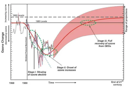
1.14 Schematic picture showing the evolution of ozone column between 60◦_{S and}

60◦_{N in 1960–2100. The red curve shows the ozone observed to date and}

projected to future and the shaded region represents the simulation results of the ozone level for the future. The green circles denote diﬀerent stages of ozone evolution (courtesy : WMO,2011). . . 18

2.1 Schematic view of the OHP lidar system (Reproduced fromGodin-Beekmann et al.,2003).. . . 26

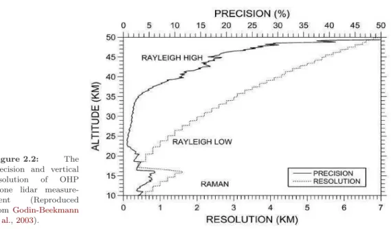
2.2 The precision and vertical resolution of OHP ozone lidar measurement (Re-produced fromGodin-Beekmann et al.,2003). . . 28

(21)

xviii List of Figures

2.3 Spectral variation of the temperature dependence of ozone cross-section from BDM (top) and BP (bottom). The wavelengths used for the DIAL ozone measurements in the troposphere and stratosphere are also marked. . . 30

2.4 Variation of ozone absorption cross-sections (BDM, original BP and the pa-rameterised BP) with respect to temperature, at 308 (top) and 331.8 nm (bottom). . . 31

2.5 Relative deviations between BP and BDM ozone cross sections at 308 and 331.8 nm with respect to temperature. . . 32

2.6 Relative diﬀerences of ozone number densities derived from the BP and BDM cross-sections at Rayleigh (308 nm) and combined Rayleigh-Raman (308+331.8 nm) wavelengths. . . 33

2.7 Vertical distribution of the annual mean of retrieved ozone from BP and BDM cross-sections at diﬀerent latitudes. The error bars represent one sigma standard deviation. . . 34

2.8 The relative diﬀerence between the old (radiosonde+CIRA) and the new (NCEP) retrievals for ozone, temperature and pressure. Error bars represent twice the standard error. . . 35

2.9 The vertical distribution of average diﬀerence in ozone measurements esti-mated using BP and BDM ozone cross-sections at OHP. . . 36

3.1 Average number of observations in each month over the respective period (top panel) and the total number of observations per year (bottom panel) of various data sets. Left: ground-based measurements at OHP. Right: satellite observations extracted around OHP. . . 45

3.2 Left: comparison of lidar measurements, both original and convolved using SBUV(/2) AKs and SBUV(/2) proﬁle on 18 September 2007 at OHP. Right: SBUV(/2) AKs used for convolving lidar data. . . 47

3.3 Vertical distribution of average relative diﬀerences of the coincident ozone measurements of various observations with lidar. Top panel: instruments with more than 10 years of data. Bottom panel: instruments with less than 10 years of data. The dotted vertical lines represent −10, 0, and 10 % and the error bars correspond to twice the standard error. Approximate pressure levels corresponding to the geometric altitudes are also shown on the right axes. . . 50

3.4 Left: Average bias between SBUV(/2) and lidar (with and without convo-lution using AKs and a priori). The number of analysed proﬁles with and without convolution are also provided in respective colours. Middle: Aver-age relative deviation of ozone from lidar and ozonesondes, with and without multiplying by correction factor. Right: Average bias from the comparison of lidar with the original and stray light corrected Umkehr. The error bars represent twice the standard error. The dashed line represents 0 % and the dotted lines represent -10 and 10%. . . 51

3.5 Comparison of lidar with the original (left panel) and stray light corrected (right panel) Umkehr ozone. The Grey and black circles represent the daily and monthly averaged diﬀerences respectively. The dashed horizontal lines represent 0 % and the dotted vertical lines represent year 1990, 1995, 2000, and 2005. . . 53

3.6 Same as Fig. 3.5, but for ozonesondes, multiplied by CF (left panel) and without multiplying by CF (right panel).. . . 54

(22)

List of Figures xix

3.7 Same as Fig. 3.5, but for SAGE II (left panel) and HALOE (right panel) with lidar. . . 55

3.8 Same as Fig. 3.5, but for SBUV(/2) with lidar, both convolved using SBUV(/2) AKs (left panel) and the non-convolved (right panel). . . 56

3.9 Monthly averaged diﬀerences of SBUV(/2) with lidar, SAGE II and Umkehr at 15.8–10 hPa. The dashed line represents 0 % and the dotted lines represent year 1990, 1995, 2000, and 2005. Data are smoothed by 3 month running mean. . . 57

3.10 Same as Fig. 3.5, but for MLS on UARS and Aura satellites (left panel) and GOMOS (right panel). The period of observations of UARS MLS and Aura MLS are shown with respective colour shades, as for Fig. 3.1. . . 58

3.11 The relative drift and twice the standard deviations estimated from the Eqs. 3.7, 3.8 and 3.10 which are denoted as σ1, σ2 and σ3 respectively, for

the comparison of HALOE with lidar. . . 59

3.12 Vertical distribution of the slopes calculated from monthly mean of the rel-ative diﬀerences of long-term (left and middle panels) and short-term (right panel) data sets with lidar data. The slopes are estimated in two periods, in 1985–2009 and 1994–2009, for the long-term data. The beginning (e.g. 1985, 1994, 2002 and 2004) and ending (2009) year of the analyses depend on the availability of the respective observations during the period. The dashed vertical line represents 0 % yr−1 _{and the error bars represent twice the}

stan-dard deviation of the slope. Approximate pressure levels corresponding to the geometric altitudes are also shown on the right axis. . . 60

4.1 Total number of profiles of all data sets at various stations (panel (a), the total number of profiles considering one measurement per day (panel (b), the total number of coincidences of different observations with lidar (panel (c) and the total number of coincidences of the long-term measurements with SBUV(/2) (panel (d), SAGE II (panel (e) and HALOE (panel (f). . . 68

4.2 Vertical distribution of the average relative differences of the coinci-dent ozone profiles of different datasets with various lidar measurements £Σ¡100 ×M eas−lidar

lidar ¢¤. The dashed and dotted vertical lines represent 0

and ±10% respectively and the error bars correspond twice the standard error. . . 71

4.3 The vertical distribution of the average error of ozone lidar and SAGE II data at various stations. . . 72

4.4 The average bias of sonde measurements, without (left panel) and with (right panel) multiplying the proﬁles by the CF, obtained for the comparison with lidar at MOHp, OHP, Tsukuba and MLO. The dotted vertical line represents 0% and the error bars correspond twice the standard error. . . 73

4.5 Vertical distribution of the slopes evaluated from the monthly averaged dif-ference time series of all observations with the lidar measurements at various regions¡100 × M eas−lidar

lidar ¢. The error bars represent twice the standard

de-viation of the slope. The dashed vertical line represents 0% yr−1 _{and the}

dotted vertical lines represent ±1.5% yr−1_. _{. . . .} ₇₄

4.6 The drifts of various lidars for the comparison with SBUV(/2), SAGE II and HALOE as references³100 ×lidar−ref_ref ´. The error bars correspond the 95% conﬁdence interval of the slope. . . 76

(23)

xx List of Figures

4.7 a) The drifts of HALOE in comparison with SAGE II as reference (see Eq. 4.2) at various stations. b) The drifts of SBUV(/2) with SAGE II as reference (see Eq. 4.2). c) Same as (b), but with HALOE as reference (see Eq. 4.3). The error bars represent twice the standard deviation of the slope. 77

4.8 The mean drifts estimated for the long-term observations with respect to other long-term measurements as references. The error bars represent twice the average of the standard deviations of the slopes obtained from diﬀerent comparisons. . . 78

4.9 Temporal evolution of the bias removed monthly averages of the relative diﬀerences of SAGE II, HALOE and Aura MLS with ozone lidar at MOHp (left panel) , OHP (middle panel) and Tsukuba (right panel). The dashed horizontal line represents 0%. . . 80

4.10 Same as Fig. 4.9, but at TMF (left panel), MLO (middle panel) and Lauder (right panel). . . 81

4.11 The drifts evaluated from the combined time series of SAGE II/Aura MLS (left) and HALOE/Aura MLS (right) at various stations. The dashed line in the left panel represents the drift of SAGE II/Aura MLS at Lauder estimated after removing the ﬁrst two measurements. The error bars represent twice the standard deviation of the slope. The dotted vertical lines represent 0 and ±0.4% yr−1_. _{. . . .} ₈₂

5.1 Time series of the monthly mean QBO at 10 and 30 hPa, solar flux, aerosol, NAO, eddy heat flux and the deseasonalised (monthly mean - mean over the period) cumulative eddy heat flux in 1980–2010. . . 88

5.2 Time series of the NAO index averaged for the winter months from De-cember to March with a 5 year moving average in black (taken from http://www.cru.uea.ac.uk/ timo/datapages/naoi.htm). . . 90

5.3 Demonstration of the PWLTs before the turnaround year (T0) and after-wards (Adapted fromReinsel et al.,2002). . . 91

5.4 The residuals obtained by filtering out the seasonal cycle, QBO, solar flux along with the PWLT (dashed line) and EESC (solid line) fits using multiple regression analysis (Reproduced fromVyushin et al., 2007). . . 91

5.5 Temporal evolution of monthly mean ozone total column measurements from the Dobson spectrometer at MOHp in 1980–2010, Dobson and SAOZ spec-trometers at OHP in 1983–2010 and 1992–2010 respectively. . . 95

5.6 Temporal evolution of monthly mean ozone anomaly from the Dobson spec-trometer at MOHp in 1980–2010, Dobson and SAOZ specspec-trometers at OHP in 1983–2010 and 1992–2010 respectively. . . 96

5.7 Time series of the relative diﬀerences of Dobson with respect to SAOZ ozone total column measurements at OHP. . . 97

5.8 Regression plot of monthly mean deseasonalised ozone from the combined Dobson and SAOZ measurements at OHP, the PW regression model and the residual (top panel), contribution from the individual proxies QBO, NAO (second panel), solar flux, heat flux (third panel) and aerosols along with the piecewise linear trend (PWLT) fit (fourth panel). . . 98

5.9 Same as Fig. 5.8, but using EESC regression model. . . 99

5.10 The inﬂuence of individual explanatory variables on the variability of com-bined Dobson and SAOZ ozone column data at OHP analysed using both PW (top panel) and EESC (bottom panel) regressions. . . 101

(24)

List of Figures xxi

5.11 The monthly PWLTs derived from the combined Dobson and SAOZ ozone total column measurements at OHP. The black and red curves represent the pre-turnaround (prior to 1997) and post-turnaround trends (after 1996) respectively. The error bars correspond to twice the standard deviation of the trends. . . 102

5.12 Same as Fig. 5.8, but for Dobson ozone column measurements at MOHp. . 104

5.13 Same as Fig. 5.9, but for Dobson ozone column measurements at MOHp. . 105

5.14 Same as Fig. 5.10, but for Dobson ozone column measurements at MOHp. 107

5.15 Temporal evolution of ozone vertical proﬁles from lidar, SAGE II, HALOE, Aura MLS and ozonesondes at OHP. The data are resolved in 1 km vertical grid. . . 108

5.16 Time series of ozone anomaly from lidar, SAGE II, HALOE, Aura MLS and ozonesondes at OHP. The data are resolved in 1 km vertical grid. . . 110

5.17 Vertical distribution of the monthly R2 _{values estimated from the PW}

re-gression model for the average data at OHP. . . 111

5.18 Vertical distribution of R2 _{estimated over the period for the average, lidar}

and SAGE II data at OHP. . . 112

5.19 Temporal evolution of the vertical distribution of average ozone anomaly (top panel), PW regression model (middle panel) and residual (bottom panel) in 1984–2010 at OHP. . . 113

5.20 Time series of the ozone anomaly, the PW regression model and the residual at 18, 21, 25, 30, 35 and 40 km calculated from the average data at OHP. . 114

5.21 Time series of the fitted signals of solar flux, heat flux, aerosols, QBO and NAO at 18, 21 and 40 km computed for the average data at OHP. . . 115

5.22 The contribution of various proxies to the variability of average ozone proﬁle at OHP. . . 116

5.23 Vertical structure of the year-round ozone trends estimated from PW and EESC functions in 15–45 km estimated from the average (left panel), lidar (middle panel) and SAGE II (right panel) data at OHP. The solid lines represent the pre-turnaround trends and the dashed lines represent the post-turnaround trends. The dotted lines represent -0.75, 0 and 0.75 %yr−1_. _{. .} ₁₁₈

5.24 Contribution of proxies to the ozone total column in DU, estimated from the average ozone vertical proﬁle at OHP. . . 119

(25)

(26)

List of Tables

3.1 Statistics of the comparison study: selection criteria in latitude (Lat) and longitude (Lon) applied for the satellite measurements with respect to OHP (43.93◦_{N, 5.71}◦_{E), time period (Year) and the maximum number of}

coin-cident proﬁles obtained seasonally [Winter (January, February, and March – JFM), Spring (April, May, and June – AMJ), Summer (July, August, and September – JAS), and Autumn (October, November, and December – OND)] and over the coincident periods (N ) with the time diﬀerence of ±12 h. 45

3.2 SBUV(/2) pressure levels corresponding to ozone column measurements, the Umkehr pressure layers and the approximate altitudes corresponding to the mid-pressure levels used in the study.. . . 48

3.3 The slope (S) and twice its standard deviation (σ) deduced from the monthly averages of the relative diﬀerences ( %) at selected altitude levels for the pe-riods 1985–2009 (S8509) and 1994–2009 (S9409). The two periods are chosen

because of the upgradation of OHP lidar in 1993. Umkehr and SBUV(/2) are given on pressure levels. . . 62

4.1 Various NDACC lidar stations, their locations and the period of observations of lidar and the analysis period of ozonesondes used in this study are given. The satellite data sets utilised for the study and their observational periods are also noted. . . 67

4.2 The RMS values estimated in 20–40 km from the average bias of each mea-surement technique at various stations.. . . 70

5.1 The piecewise linear trends before (CT 1) and after (CT) 1997 and the

re-gression coefficients of QBO 10, QBO 30, aerosol, solar flux, NAO and heat flux, estimated from the combined Dobson and SAOZ ozone total column measurements at OHP are shown for March, September and the average of all months. CT 1and CT are given in DU/year, aerosol, NAO and heat flux

are given in DU, QBO 10 and QBO 30 are expressed in DU/(m/s) and solar ﬂux is in DU/(100 SFU). Twice the standard deviation of the trends and regression coeﬃcients are given in the parentheses. . . 97

5.2 The interannual variability of ozone total column measurements in DU, es-timated for each month at OHP and MOHp. . . 100

5.3 The year-round pre-turnaround and post-turnaround trends, and twice the standard deviation estimated using both PW and EESC regressions for OHP and MOHp. Trends and standard deviations are shown in DUyr−1_._{. . . . .} ₁₀₃

(27)

(28)

Chapter 1

Introduction

1.1 Vertical structure of the atmosphere. . . 1 1.2 Stratospheric ozone . . . 2 1.2.1 Stratospheric chemistry . . . 3 1.2.2 Dynamical processes . . . 5 1.3 Ozone depletion issue . . . 7 1.3.1 Antarctic ozone loss . . . 7 1.3.2 Arctic ozone loss . . . 11 1.3.3 Mid-latitude ozone loss . . . 12 1.4 Equivalent Effective Stratospheric Chlorine. . . 13 1.5 Present state of the ozone layer. . . 14 1.5.1 Ozone total column measurements . . . 14 1.5.2 Ozone vertical proﬁle . . . 15 1.6 Ozone recovery : different stages of ozone evolution . . . 17 1.7 Ozone and climate . . . 18 1.8 Conclusions . . . 19

This thesis discusses the evolution of stratospheric ozone measured from various ground and space-based observations over the middle and subtropical NDACC (Network for the Detection of Atmospheric Composition Change) lidar (Light Detection And Ranging) sta-tions. Therefore, a brief introduction of the chemical and dynamical processes that affect the distribution of ozone in the stratosphere is presented in this chapter, to follow the later sections and discussions on the ozone evolution. Section 1.1 describes different layers of the atmosphere and the temperature distribution. A detailed description of stratospheric chemistry and dynamics involved in the production, distribution and destruction of strato-spheric ozone is given in Section 1.2. The chemical and dynamical processes associated with the rapid destruction of ozone is discussed in Section 1.3 followed by the measure-ments of the stratospheric ozone destruction in Section 1.4. Section1.5presents a review of stratospheric ozone column and profile trends and described the different stages of ozone evolution. Then, a link between ozone and climate is discussed in Section 1.7. Finally, Section1.8concludes the general description and presents the objectives of the study.

1.1 Vertical structure of the atmosphere

The atmosphere is divided into diﬀerent layers from the ground to 100 km based on the distribution of temperature. Figure 1.1 illustrates a schematic representation of various layers in the atmosphere, namely the troposphere, stratosphere, mesosphere and thermo-sphere. Each layer is distinct with respect to its temperature distribution. The tropopause separates troposphere and stratosphere, stratopause divides stratosphere and mesosphere

(29)

2 Chapter 1. Introduction

Figure 1.1: Schematic representation of the thermal structure of the atmospheric temperature based on the US Standard Atmosphere (1976).

and mesopause is the boundary between mesosphere and thermosphere. The temperature decreases with altitude in the troposphere and the tropopause decreases in altitude from the tropics to the poles and varies with respect to seasons. On average, it ranges between 8 km in the polar latitudes, 15 km in the mid-latitudes and 17 km in the tropics. The tropopause varies from ∼7 km in winter to ∼9 km in summer in the poles, from ∼12 km in winter to ∼18 km in summer in the mid-latitudes and from ∼15 km in winter to ∼20 km in summer in the tropics. All weather phenomena (e.g. clouds, rains etc.) take place in the troposphere. The region above tropopause to about 50 km is called the stratosphere, where temperature increases with height and is the focus of the present study. So the re-gions above the stratopause are not discussed here. The region above the tropopause until ∼110 km is termed as the middle atmosphere (Andrews et al.,1987).

1.2 Stratospheric ozone

Ozone, made up of three oxygen atoms is a minor constituent (0.000004 %) in the atmo-sphere. The ozone was first identified in the laboratory by Christian Fredrich Schönbein in 1840 and the presence of ozone in the air was first detected by André Houzeau in 1858 (Brasseur, 2008). Since then, routine research has been going on to measure the atmo-spheric concentration of ozone. Studies revealed that most of the ozone is confined to the stratosphere. Maximum ozone concentration and mixing ratio are found near 22 and 35 km respectively, depending on latitude and season. Ozone absorbs the harmful ultraviolet ra-diation (UV), particularly UV-B (280–315 nm) and UV-C (100–280 nm), and thus acting as a heat source responsible for the temperature positive gradient in the stratosphere. This is the only gas in the atmosphere that absorbs UV-B radiation and hence, it is considered as a vital atmospheric constituent that helps to keep life on the Earth.

Stratospheric ozone can be measured as both vertical proﬁle and total column. General form of the measured quantities are volume mixing ratio (VMR) in parts per million by volume (ppmv), number density in molecules/ cm3_{, partial pressure in mPa and Dobson}

(30)

1.2. Stratospheric ozone 3

equivalent to the thickness of the ozone layer at standard temperature (0◦_{C) and pressure}

(1013.25 mb). It is about 3 mm or 300 DU (8×1022_{molecules/ m}2_{) for a column containing}

the global mean amount of ozone (Andrews et al., 1987), where 1 DU=10−2_{mm and}

1 DU=2.69×1016_{molecules/ cm}2_.

The mathematical formulations of the units are :

1 DU = dA × 1 O3 × 10 14_×_V NA 1 molecules/cm3 = 1 V M R T × 1.38 × 10−19 1 molecules/cm3 = 1P P 1.38 × 10−14

where mm is millimeter, dA is diﬀerence in altitude in meter (m), O3 is ozone in molecules/m3_, V is volume of ideal gas at standard temperature and pressure (22.4 m3_{/kmol), N}

A is Avogadro’s Number (6.022×1026_{/kmol), VMR in ppmv, P is pressure in hPa, T is temperature in Kelvin (K)} and PP is ozone partial pressure in milli-Pascal (mPa).

1.2.1 Stratospheric chemistry

The stratospheric ozone chemistry involves both production and natural destruction of ozone. In the stratosphere, these processes are dominated by photochemical reactions. A photochemical model for the vertical distribution of ozone in the stratosphere was ﬁrst formulated by Chapman, known as the Chapman mechanism (Chapman,1930). According to Chapman reactions, ozone is produced by the photodissociation of oxygen molecule (O2)

by UV-radiation. That is,

O2+ hν → O + O λ ≤ 242 nm (1.1)

O + O2+ M → O3+ M (1.2)

where M is an inert air molecule stabilizing the reaction by removing excess energy.

The photochemical production of ozone is balanced by its loss through the photolytic pro-cess.

O3+ hν → O2+ O(3P ) λ ≤ 1100 nm (1.3)

O3+ hν → O2+ O(1D) λ ≤ 320 nm (1.4)

O + O3 → 2O2 (1.5)

O + O + M → O2+ M (1.6)

However, Chapman’s ozone chemistry was not suﬃcient to explain the actual amount of ozone present in the stratosphere, which is lower than that predicted in Chapman mecha-nism. Later, it is reported that the stratospheric ozone was destroyed not solely by atomic oxygen, but several catalytic mechanisms are also involved in the natural ozone removal process, i.e.,

X + O3 → XO + O2 (1.7)

XO + O → X + O2 (1.8)

(31)

where X is a catalyst, which is not consumed in the process. The catalysts are hydrogen (H), hydroxyl radical (OH), nitrogen oxide (NO), chlorine (Cl) and bromine (Br).

The catalytic reactions caused for the destruction of ozone are:

a) Hydrogen catalytic cycle : Bates and Nicolet (1950) discovered that the oxidation of water vapour produces OH, which plays a critical role in destructing ozone as a direct reactant or helps other ozone destruction reactions.

H2O + O(1D) → 2OH (1.10) O + OH → O2+ H (1.11) H + O2+ M → HO2+ M (1.12) O + HO2 → O2+ OH (1.13) N et : O + O + M → O2+ M (1.14) OH + O3 → HO2+ O2 (1.15) HO2+ O3 → OH + 2O2 (1.16) N et : 2O3 → 3O2 (1.17)

b) Nitrogen catalytic cycle : The reaction with nitrogen oxides could represent a signiﬁcant sink for ozone in the stratosphere (Crutzen,1971) .

N O + O3 → N O2+ O2 (1.18)

O + N O2 → N O + O2 (1.19)

N et : O + O3 → 2O2 (1.20)

c) Chlorine catalytic cycle : Stolarski and Cicerone(1974);Molina and Rowland(1974) pointed out that the rising atmospheric concentrations of chloroﬂuoromethanes produces a signiﬁcant amount of Cl in the stratosphere. It undergoes a catalytic reaction that destructs ozone.

Cl + O3 → ClO + O2 (1.21)

ClO + O → Cl + O2 (1.22)

N et : O + O3 → 2O2 (1.23)

The reaction 1.22 is faster than the reaction 1.19. So reaction 1.22 is more eﬃcient in destroying ozone.

The destruction rate of ozone by diﬀerent catalytic cycles varies depending on altitude and latitude. Figure 1.2 illustrates the relative contribution of diﬀerent reactions in de-stroying ozone at various latitudes and altitudes. The Figure shows that the NOX cycle is

dominant in the middle stratosphere and amounts to >50 % at all latitudes. The contri-bution of HOX cycle is the largest (50–90 %) in the lower and upper stratosphere without

any latitudinal diﬀerence. The Cl cycle plays an important role in 20–30 and 35–45 km, contributing to about 30 % while Br cycle provides its maximum (20–50 %) in the lower stratosphere at high latitudes in the southern hemisphere (SH) and ∼10 % in the lower stratosphere of the equator and in the northern hemisphere (NH).

So ozone equilibrium is a consequence of creation and destruction processes. The pho-tochemical production of ozone is favourable in the 200–242 nm range, the wavelength that can penetrate up to the lower stratosphere. Since UV radiation is highest in the tropics, maximum ozone is produced there, with the expected maximum in summer and minimum

(32)

1.2. Stratospheric ozone 5

Figure 1.2: Vertical distribution of the relative contribution of various reaction cycles in depleting ozone at various latitudes (fromBrasseur et al.,1999).

in winter. Nevertheless, the observed behaviour is very diﬀerent from this theoretical frame-work since most ozone is found in the mid to high latitudes with the highest levels in spring and the lowest in autumn while the lowest values are located in the tropics, as shown in Fig.1.3.

Hence, it is clear that although ozone is produced from the photochemical reactions, its global distribution in the atmosphere is driven by atmospheric motions transporting ozone from its source region in the tropics to the high latitudes. These processes are described in the following section.

1.2.2 Dynamical processes

The discrepancy between the photochemical theory and observations in the distribution of ozone can be explained by the transport processes in the atmosphere. The transport of ozone from the tropical source regions to the middle and high latitudes is mainly responsible for the observed high ozone amounts in those regions. The transport processes are sensitive to temperature and pressure. Because of the high solar radiation in the tropical regions, the air warms, converges and rises through the tropical upwelling and creates a low pressure system in the equator. When it reaches upper part of the troposphere (10–15 km), it is forced to turn and moves horizontally toward the north and south poles. A portion of the air cools and sinks at about 30◦_{N/S, resulting in a high pressure system in the subtropics.}

(33)

Figure 1.3: Monthly mean ozone total column abundance in DU from the TOMS observations averaged in 1979–1986 as function of latitude and season (fromBrasseur et al.,1999).

Because of this pressure gradient (the subtropical high and equatorial low), air close to the surface moves from the subtropics to the equator. This circulation pattern of air is known as Hadley cell. The portion of air moving from the subtropics to the equator is deﬂected towards the west from east by the Coriolis force and is called tropical easterlies. The other portion of air close to the tropopause moving from the subtropics to the poles produces westerlies.

Air parcels from the troposphere enters the stratosphere in the tropics, moves towards the winter pole over a period of years and returns to the troposphere in the extratropics. This vertical transport controlled by the large-scale diabatic circulation is referred to as the Brewer-Dobson (BD) circulation in honour of the eminent atmospheric scientists, Brewer and Dobson. Because, using this mean meridional circulation Brewer explained the observed low water vapour mixing ratios in the stratosphere (Brewer,1949) and Dobson pointed out the observed high ozone concentration in the polar lower stratosphere (Dobson, 1956). Schematic outline of the BD circulation is shown in Fig.1.4. BD circulation consists of two meridional cells in each hemisphere with rising motion in the tropics, poleward flow at mid-latitudes and sinking motion in the polar regions. The summer stratosphere is characterised by the mean easterly flow while the winter stratosphere by mean westerly flow. During winter, the tropospheric wave disturbances propagate upward into the stratosphere, where they break and dissipate due to wave breaking processes (Haynes,2005). This dissipation leads to a drag acting in the opposite direction to the westerly flow. Since the Earth is rotating, the Coriolis force, which is maximum in the poles, balances this drag and produces a poleward motion.

(34)

1.3. Ozone depletion issue 7

Figure 1.4: Schematic representation of the stratospheric circulation (fromHolton et al.,1995).

1.3 Ozone depletion issue

Apart from the natural destruction of ozone, as mentioned in Sect.1.2.1, the stratospheric ozone depletion is further enhanced by the higher levels of Cl and Br containing compounds emitted by the human activities. These halogen source gases of anthropogenic origin con-trolled under the Montreal Protocol are referred to as ozone depleting substances (ODSs). They include chloroﬂuorocarbons (CFCs), hydrochloroﬂuorocarbons, (HCFCs), brominated CFCs (halons), carbon tetrachloride (CCl4), methyl chloroform (CH3CCl3) and methyl

bro-mide (CH3Br) (WMO, 2007, 2011). These emissions accumulate in the troposphere and

are transported to the stratosphere, where they convert to reactive halogen gases by UV radiation and increases the ozone depletion. The degradation of ODSs in the stratosphere releases Cl and Br atoms, which are readily combined to form inorganic Cl (Cly) and

inor-ganic Br (Bry) compounds. Since CFCs and halons are more stable and are not decomposed

in the troposphere, their use leads to an increase in the concentration of Cl and Br in the stratosphere. The most abundant Cly reservoirs are HCl and ClONO2 and Bry reservoirs

are HBr and BrONO2. These reservoirs are transformed to active Cl or Br and thus deplete

stratospheric ozone. The studies (Daniel et al., 1999; Sinnhuber et al., 2009) reveal that the potential for ozone depletion by Br is signiﬁcantly larger (∼40–100) than that by Cl as the Bry reservoirs are less stable than their Cly counterparts.

1.3.1 Antarctic ozone loss

In 1985, a path-breaking study byFarman et al.(1985) announced a dramatic loss of ozone column in spring at the Halley-Bay station, in the Antarctic. It was later conﬁrmed by satellite measurements and in other Antarctic regions too. The ozone proﬁle measurements by ozone sounding (Chubachi, 1984) revealed that the loss was severe in the 12–21 km altitude range. A complete loss of ozone (saturation of ozone loss) at this altitude region was observed since early 1990s too. This ozone layer having less than 220 DU was termed

(35)

(36)

as the Antarctic ozone hole. Figure 1.5 demonstrates the Antarctic ozone hole in 2006, the largest one (∼56 %) ever observed in the Antarctic stratosphere, in comparison with that in 1981. The ozone loss chemistry, described previously, was not suﬃcient to explain very rapid loss in the Antarctic. Because in the low light conditions the concentration of oxygen atoms (O) is very low. Therefore, the reactions requiring O were no longer eﬀective there. Several theories including dynamics and chemistry were put forward for explaining this ozone loss in the polar lower stratosphere.

Figure1.6shows diﬀerent steps leading to the depletion of ozone in the Antarctic. First, chemically active clouds in the stratosphere called polar stratospheric clouds (PSCs) are formed inside the extremely persistent Antarctic polar vortex during very cold condition, when temperature reaches below 195 K. Second, heterogeneous reactions occur on the sur-faces of PSCs releasing active Cl2 from its reservoirs (Solomon et al., 1986) and produces

HNO3 from NO and NO2. The removal of NO and NO2 reduces the possibility to reform

ClONO2 or BrONO2. Third, Cl2 undergoes photolysis and produces Cl when sunlight

returns. Fourth, ozone destruction occurs through catalytic reactions with Cl. First and second processes need darkness while third and fourth steps occur in the presence of sun-light. A detailed description of these processes are given below.

Figure 1.6: Schematic diagram showing various chemical and dynamical processes involved in the destruc-tion of ozone in the Antarctic polar vortex (source : Brasseur et al.,1999).

Several cycles not involving oxygen atoms were proposed after the discovery of ozone hole for explaining the chemical polar ozone loss. One mechanism involves Br radicals, as reported byMcElroy et al.(1986).

BrO + ClO → Br + Cl + O2 (1.24) BrO + ClO → BrCl + O2 (1.25) BrCl + hν → Cl + Br (1.26) Cl + O3 → ClO + O2 (1.27) Br + O3 → BrO + O2 (1.28) N et : 2O3 → 3O2 (1.29)

(37)

Another catalytic cycle found to be important for the ozone destruction in the Antarctic lower stratosphere is the one involved with chlorine monoxide (ClO) dimer proposed by Molina and Molina(1987). High amount of ClO triggers a new catalytic reaction involving a self reaction of ClO, which is caused for the signiﬁcant ozone loss.

ClO + ClO + M → Cl2O2+ M (1.30)

Cl2O2+ hν → Cl + ClO2 (1.31)

ClO2+ M → Cl + O2+ M (1.32)

2[Cl + O3 → ClO + O2] (1.33)

N et : 2O3 → 3O2 (1.34)

The net reaction in the two cases is the destruction of two ozone molecules forming three oxygen molecules. Studies have shown that contribution of the chemical cycles ClOX

and BrOX to the ozone loss is about 40–45 and 35–40 %, respectively in June–mid-October

(Marchand et al., 2005; Kuttippurath et al., 2010). These reactions occur in the pres-ence of visible light only. So ozone destruction due to these reactions takes place in the winter/spring, when sunlight returns to the polar stratosphere. During the term, late winter/early spring, the UV radiations are weak and hence, ozone production does not happen. Hence, if suﬃcient amount of ClO is generated in the atmosphere, these reactions can explain most of the ozone loss found over Antarctica. Large amount of ClO has been originated from the reactions taking place on the PSCs and are described below.

Figure 1.7:Schematic view of PSC in the Antarctic stratosphere (source : NASA).

1.3.1.1 PSCs and heterogeneous chemistry

Normally, the stratosphere is very dry and cloudless even though a thin layer of aerosol (liquid-phase binary H2SO4/H2O droplets) is present in the lower stratosphere. But during

polar night, when temperatures reach below 195 K in 15–25 km the background aerosols take up HNO3 and H2O and evolve into ternary HNO3/H2SO4/H2O droplets, referred to

as PSCs (Carslaw et al.,1994). Figure1.7shows a photograph of the PSCs in the Antarctic stratosphere. PSCs are classiﬁed into three types, Type Ia, Type Ib and Type II, according to their physical state or optical properties and chemical composition. This classiﬁcation is based on air-borne lidar measurements (lidar backscatter and depolarisation ratios for PSCs) as the instrument is sensitive to the state of polarisation of the backscattered light

(38)

(Browell et al., 1990; Felton et al., 2007). Type Ia PSCs are made up of crystals of ni-tric acid trihydrate [NAT - (HNO3. 3H2O)] and Type Ib consists of supercooled ternary

solutions (STS) of HNO3/H2SO4/H2O. Type II PSCs are frozen water ice non-spherical

crystalline particles. During austral winter heterogeneous reactions occur on the surface of PSC particles and convert the reservoir species such as ClONO2 and BrONO2 into more

active species. The principal heterogeneous reactions are given below.

HCl(s) + ClON O2(g) → HN O3(s) + Cl2 (1.35)

BrON O2(g) + H2O(l) → HN O3(g) + HOBr(g) (1.36)

HCl(s) + BrON O2(g) → HN O3(g) + BrCl(g) (1.37)

HCl(l) + HOBr(g) → H2O(l) + BrCl(g) (1.38)

Other heterogeneous reactions occurring on the surfaces of PSCs releasing Cl2 are

ClON O2(g) + H2O(s) → HN O3(s) + HOCl(g) (1.39)

HCl(s) + HOCl(g) → H2O(s) + Cl2(g) (1.40)

Another heterogeneous reaction releasing photolytically active Cl2 by the photolysis of

ClNO2is

N2O5(g) + HCl(s) → ClN O2(g) + HN O3(s) (1.41)

However, for the production of Cl atoms sunlight is required. When the sun starts to shine on the polar stratosphere at the beginning of austral spring, Cl2 is photolysed

to Cl, that enters into catalytic destruction of ozone. This is the reason why ozone is depleted in spring, when sunlight returns. Thus, above reactions accumulate the ClO concentration in the polar lower stratosphere, which then initiate the ozone destruction cycle (Reactions1.30–1.34).

1.3.2 Arctic ozone loss

Figure 1.8:Total ozone average in March and October in the northern and southern hemispheres, respec-tively. The horizontal Gray lines are the average total ozone prior to 1983 in March (NH) and October (SH) and the symbols represent the satellite data in different years.