Must the random man be unrelated? A lingering misconception in forensic genetics

1 2 3 4 5

Must the random man be unrelated? A lingering misconception about forensic

genetics

POSTPRINT VERSION. The final version is published here:

Milot, E., Baechler, S., & Crispino, F. (2020). Must the random man be unrelated? A lingering misconception in forensic genetics. Forensic Science International: Synergy, 2, 35-40. http://dx.doi.org/10.1016/j.fsisyn.2019.11.003 CC BY-NC-ND 4.0

Abstract

25

A nearly universal practice among forensic DNA scientists includes mentioning an unrelated

26

person as the possible alternative source of a DNA stain, when one in fact refers to an unknown

27

person. Hence, experts typically express their conclusions with statements like: “The probability

28

of the DNA evidence is X times higher if the suspect is the source of the trace than if another

29

person unrelated to the suspect is the source of the trace.” Published forensic guidelines

30

encourage such allusions to the unrelated person. However, as the authors show here, rational

31

reasoning and population genetic principles do not require the conditioning of the evidential

32

value on the unrelatedness between the unknown individual and the person of interest (e.g. a

33

suspect). Surprisingly, this important semantic issue has been overlooked for decades, despite its

34

potential to mislead the interpretation of DNA evidence by criminal justice system stakeholders.

35 36

Keywords: DNA evidence; fact-finder; match probability; relatedness; semantics

37 38

1. Introduction

39

Forensic science has been the target of severe critiques, in particular through the reports of the

40

National Research Council in 2009 [1] and the President’s Council of Advisors on Science and

41

Technology in 2016 in the USA [2]. DNA typing was relatively spared by that storm, largely due

42

to its strong grounding in probabilistic models to assess the weight of evidence. Nevertheless, the

43

rendering of the weight of DNA evidence may mask fundamental interpretation issues for

fact-44

finders, where semantics and communication are of prime importance. As highlighted by a

45

growing body of research [3-10], communication between scientists and non-scientists is far from

46

straightforward and may cause unconscious misunderstandings. Each word is important and the

47

burden is on forensic scientists to convey their message in an accurate, transparent, readable and

48

efficient way. Many debates between law and forensic science experts1 _{underline the semantic}

49

1 Such as for instance the interdisciplinary symposium held during the 69th _{American Academy of Forensic Sciences}

conference in New Orleans (USA) in 2017. In this symposium, presentations and a panel discussion bringing together judges, prosecutors, forensic scientists and academics brought out that forensic scientists must improve in expressing clearfully their results in reports and in court hearings, in particular when it comes to competing hypotheses their wording and what they encompass must be transparent for all stakeholders and dispel any blur whether conscious or not.

issues and call to set up solutions for a clear communication that removes any ambiguity, a sort

50

of common language between science and justice.

51 52

One semantic issue that has lingered ever since the introduction of trace DNA analyses in

53

criminal investigations pertains to a very widespread practice: the concept of the ‘unrelated

54

person’. Experts typically express their conclusions about the weight of DNA evidence with

55

statements like: “The probability of the evidence is X times higher under the hypothesis that the

56

suspect is the source of the trace than under the hypothesis that another person unrelated to the

57

suspect is the source of the trace.” The word ‘unrelated’ has spreaded across the forensic

58

literature since its tentative appearance in Jeffreys et al.’s initial paper on DNA fingerprints [11].

59

Nowadays, the word is almost always present in expert reports, scientific papers, textbooks and,

60

importantly, forensic guidelines and recommendations. For instance, in the ENFSI Guideline for

61

Evaluative Reporting in Forensic Science, DNA case examples mention alternative propositions 62

considering “an (unknown) unrelated person” [12, pp. 34, 40]. Likewise, in its latest

63

recommendations the DNA commission of the International Society of Forensic Genetics

64

mentions "it is standard to apply the ‘unrelated’ caveat" (see footnote 6 in ref. [13]).

65 66

While there is an abundant literature about the problem of how to deal with relatives in forensic

67

genetics, curiously we found no published reference that fundamentally addresses the

68

interpretation of the concept of ‘unrelatedness’. This issue is semantic in nature and does not

69

challenge the validity of the mathematical models that are applied to assign the probability of

70

DNA evidence in everyday casework. However, we are concerned about the confusion that the

71

routine and default usage of the word ‘unrelated’ can cause among an audience of investigators,

72

lawyers, prosecutors or fact finders over the correct meaning of calculations pertaining to DNA

73

evidence.

74 75

2. Confusion over the ‘unrelated’

76

All individuals have relatives. This is a consequence of the finite size (N < ∞) of populations.

77

Thus, suspects have relatives too. The more genes they share with them, the more challenging it

78

may be to make conclusive inferences about the source of DNA traces. This explains why

79

forensic experts tend to specify that the reported weight of evidence holds only if the source of

80

the trace is unrelated to the suspect or, equivalently, that the suspect’s relatives are excluded from

81

the pool of individuals that may be randomly drawn from the population of interest. However,

82

since an individual is always related to any other member of the population – whether their most

83

recent common ancestor lived one generation or thousands of years ago, conditioning on

84

unrelatedness implies that the weight of evidence strictly applies to a non-existent fraction of the

85

population. No doubt that forensic scientists have a more practical definition in mind when they

86

use the word ‘unrelated’, such as “not closely related to the suspect” or “not related to a degree

87

close enough to bias substantially the calculation of the weight of evidence”. Yet, such fuzzy

88

definitions can be misleading.

89 90

First, referring to a person unrelated to the suspect may be perceived as if the population of

91

interest excluded (close) relatives, in a sense a form of covert exoneration2_{. This is because, in}

92

such a case, the set of people encompassed by the prosecution and the defence hypotheses

93

excludes relatives, which may give the impression that both sides do not consider them as

94

relevant. Second, one may think that relatives compromise the value of evidence. For instance, as

95

suggested by a reporting scientist with who we discussed the issue, one may wonder if the use of

96

the word ‘unrelated’ in the alternative proposition means that if the suspect has a brother, the

97

weight of evidence is meaningless and the DNA evidence useless. Third, non-geneticists may

98

think that two persons that do not fall under a usual “close relationship” category are necessarily

99

2 Indeed, background case information is most of the time insufficient or unavailable to assume such exclusion. This

is not the role of the forensic scientist alone, who is left in most cases with a great deal of uncertainty about the relatedness factor. It may be tempting to reduce uncertainty by gathering circumstantial information about existing relatives through further investigations, by querying administrations or by asking directly the suspect. However, such information can rarely be considered as fully reliable and comprehensive. For instance, the suspect could state in interviews that he has brothers when in fact he has none. Administrative registers, when they exist, may be incomplete in particular about foreigners, and they provide official family relationships that do not always reflect biological relationships (e.g., illegitimate children) and certainly do not cover the full range of close to remote relationships. Finally, putting aside the impact on efficiency and timeliness for the case in process, one may also claim against bias of the forensic scientist's interpretation when gathering further circumstantial information.

more genetically distant than close relatives. Take the example of first cousins. Their kinship

100

coefficient3 _{() is 0.0625. However, in theory there are a plethora of pedigree relationships that}

101

can lead to the exact same kinship level when two persons share several but more remote

102

ancestors, especially in endogamous populations.

103 104

Actually, forensic biologists do not seem to agree on the correct interpretation of ‘unrelated’. The

105

issue arouse independently to authors of this paper in different contexts in Europe and North

106

America, demonstrating similar concerns about the word ‘unrelated’ shared by practitioners and

107

researchers in various countries. For example, in a 2012 international workshop on forensic

108

DNA, one of us suggested that the word ‘unrelated’ should not be used anymore in expert

109

reports. The discussion that followed among reporting scientists showed that they diverge over

110

the interpretation and implications of this term. The issue was also brought forward in 2017

111

within a Swiss working group dedicated to interpreting forensic evidence and expressing

112

conclusions. Despite admitting discomfort when asked to justify the default use of the word

113

‘unrelated’, the members decided to keep using it until the scientific literature addresses the

114

question because, if questioned, they must refer to "the scientific state of knowledge".

115 116

Moreover, the concept of unrelatedness, as applied in forensic science, disagrees with population

117

genetic principles. Essentially, the problem arises when the absence of knowledge about the

118

relatives of a person of interest leads the scientist to transform the ‘unknown person’ (the 119

classical ‘random man’) into an ‘unrelated person’ upon reporting a random match probability, a

120

likelihood ratio, or any other quantitative assessment of the DNA evidence. However, the key

121

point for the correct interpretation of the weight of DNA evidence is not the existence of relatives

122

per se but rather the information that one has or not about them and about their potential 123

involvement in the case at hand. As we show in the next section, when no information about

124

relatives is available/used, it is appropriate to apply standard equations based on the

Hardy-125

Weinberg (HW) law without conditioning the weight of evidence on the unrelatedness between

126

the person of interest (e.g. suspect) and the source of the trace.

127

3 _{The kinship coefficient is defined as the probability of randomly drawing from different individuals two alleles that}

3. All is relative

128

Consider two competing hypotheses about the source of a trace, Hp and Hd, respectively proposed 129

by the prosecution and the defence [14]. In a Bayesian framework, the strength of our belief in

130

favour of one hypothesis over the other before observing the DNA evidence (i.e. the ratio of their

131

prior odds), is given by Pr(Hp|I)/Pr(Hd|I), where I is any other relevant (e.g., circumstantial) 132

information available about/for the casework. After observing the DNA evidence (E), the

133

posterior odds become

134 135 Pr(𝐻_𝑝|𝐸, 𝐼) Pr(𝐻_𝑑|𝐸, 𝐼) = Pr(𝐸|𝐻_𝑝, 𝐼) Pr(𝐸|𝐻_𝑑, 𝐼)× Pr(𝐻_𝑝|𝐼) Pr(𝐻_𝑑|𝐼) 136 137

where Pr(𝐸|𝐻𝑝, 𝐼)/Pr(𝐸|𝐻𝑑, 𝐼) is the likelihood ratio (LR). In equation (1), case information

138

available about relatives is a component of I and we will designate it by IR. A classical example is 139

when the suspect has a brother who is assumed to belong to the population of interest. In such a

140

case, Hp usually remains unchanged (e.g. “the suspect is the source of the trace”) while Hd could 141

be that “his brother is the source of the trace”, or that “another person other than the suspect, not

142

excluding his brother, is the source”. In either case the calculation of the LR denominator must be

143

adjusted appropriately [15]. Therefore, changing IR can modify or refine both the set of 144

hypotheses to be evaluated and the calculation of the LR, in agreement with these hypotheses

145

[16]4_{. Now, since this is true for any defence hypothesis admitting any specified relatives as the}

146

alternative source of the DNA stain [15, 18], we will not limit our consideration to the sole

147

brother case and refer more generally to the kinship coefficient , which has a value for every

148

degree of genetic relationship (see footnote 3).

149 150

When the reporting scientist has no knowledge about the existence of relatives, then IR =  151

(empty set). In this case, it is generally assumed that the calculation of Pr(𝐸|𝐻𝑑, 𝐼) in equation

152

(1), which is based on Hardy-Weinberg law in the simplest model, holds only when the source is

153

4 Concerning the assessment of multiple hypotheses in the LR calculation, we refer the reader to Buckleton et al. [17]

J.S. Buckleton, C.M. Triggs, C. Champod, An extended likelihood ratio framework for interpreting evidence, Science and Justice 46(2) (2006) 69-78.

unrelated to the suspect, that is  = 0 (with Hd defined accordingly). However, this is a mistake 154

because the only thing that the calculation in the denominator entails is that the reporting scientist

155

incorporates no relevant information about the kinship of the suspect to other persons in the

156

population. That is, IR =  does not imply Pr( > 0) = 0, i.e. that individuals are totally unrelated. 157

Strictly speaking, an absence of kinship between individuals is expected only in infinite

158

populations since Pr( > 0)  0 when N  ∞ under random mating [19]. Consequently, the

159

absence of information cannot be equated to an absence of kinship since an individual is always

160

related somehow to any other member of the finite population.

161 162

The use of the word ‘unrelated’ is even more problematic under the Balding-Nichols (BN) model

163

[20], which is routinely applied by forensic labs in place of the HW model. This model postulates

164

that relatedness does exist between the suspect and the source of the trace due to population

165

subdivision, such that individuals from the same subpopulation share a common ancestry. The

166

theta (θ) parameter of this model corrects for the non-independence of their genetic profiles by

167

incorporating information from population genetic studies. Obviously, this means that IR ≠  and 168

that the probability of kinship between the suspect and other persons from the same

169

subpopulation (Pr( > 0)) is greater than zero. Consequently, it is incoherent to use the word

170

‘unrelated’ in the formulation of the weight of evidence based on this model.

171 172

Moreover, contrary to common admittance, HW or BN equations do provide correct values for

173

the probability of a genetic profile when one admits the possible inclusion of the suspect’s

174

relatives in the population of interest, as long as no information about these relatives is available,

175

as demonstrated for the HW case in Appendix A. Hence, the standard random match probability

176

must be understood as the match probability in the absence of knowledge about relatives, rather

177

than in its common but wrong acceptance as the “match probability when no relatives exist”. A

178

similar reasoning applies to other forms of weight-of-evidence metrics that tend to refer to

179

unrelated persons in their verbal formulations, including LRs of various degree of sophistication.

180 181 182

4. The unrelatedness concept: an unnecessary burden

183

To circumvent the lack of precision conveyed by reference to unrelated individuals, some authors

184

proposed to change the calculation and presentation of the weight of evidence. In their “call for a

185

re-examination of reporting practice”, Buckleton and Triggs [16] concluded that “it is time that

186

the match probabilities for a sibling are reported in all casework involving many loci where the

187

suspect has a non-excluded sibling” – a call that however appears to have had little effect on

188

current common DNA reporting practice (see [21] for a similar argument). Likewise, Taylor et al.

189

[22] proposed a “unified LR” that accounts for potential relatives and “removes the need to

190

stipulate that the alternative donor is unrelated when forming the propositions” [22, p. 57]. 191

Basically, LRs considering different types of relatives are calculated, weighted by the postulated

192

frequency of each type of relative, and then summed up (i.e., considering that IR ≠  at 193

population level) [22]. The STRmix™ software lets the user specify the average number of

194

children per family (i.e., IR ≠ ), to better reflect the composition of the population of interest 195

(see http://strmix.esr.cri.nz/#home for a list of publications relative to the methods implemented

196

in STRmix™). As far as the assumptions about the relatedness structure are made explicit, above

197

approaches have the advantage of considering populations that are more realistic of human

198

mating systems than the classic ‘random mating’ scheme. However, while they address the

199

problem of how to best quantify the weigh of evidence, they do not address the semantic issue of

200

their verbal formulation. Indeed, they do not totally eliminate the use of the word ‘unrelated’

201

because an ‘unrelated’ category may still remains among the several types of relatives

202

considered. What should we do then?

203 204

First, we suggest to simply consider that if the unknown individual who left a DNA trace

205

happened to be the brother or the cousin of the suspect, this would be a sort of ancillary

206

consequence, a way by which we categorize and name one among many possible genetic

207

outcomes of a random draw (the source of the DNA trace under the defence hypothesis) in a

208

finite population. This way of expressing the relatedness avoids the pitfalls associated with the

209

choice of an arbitrary definition of ‘unrelated’ within the forensic context. Second, referring

210

simply to an “unknown person” or to the “random individual” is sufficient because one should

211

not (and doesn’t need to) discard the possibility that the source is related to the suspect to an

unknown degree. Alternatively, a more explicit wording would be “an unknown person, without

213

regard to his relatedness to the suspect”. Again, the important point here is not unrelatedness but

214

the absence of relevant knowledge about relatives (IR = ), which prevails in most real life 215

caseworks. Critically, in assessing the weight of the DNA evidence with standard metrics, one

216

must nevertheless bear in mind the assumption that the suspect has no more or less chance to

217

have relatives of a given degree than the average person in the population of interest. Therefore,

218

it is still important to specify that potential relatives are included in the list of possible donors,

219

especially when the set of possible suspects is small.

220 221

5. Conclusion

222

The arguments presented in this paper call for a change in reporting practices to prevent semantic

223

confusion and potential misinterpretation of DNA evidence by fact-finders and other criminal

224

justice system participants. We suggest avoiding the routine and default use of the word

225

‘unrelated’, not only in oral communications and expert reports, but also in the forensic literature

226

in general, including guidelines and recommendations. Some might believe that this issue is

227

unlikely to have a big influence on the interpretation of forensic DNA expertises. We doubt it is

228

the case, considering the confusion that exists even among reporting scientists (see section 2).

229

There is a vacuum in the literature about this question that needs to be filled. Thus, we hope this

230

paper will spark discussion, and will be glad to hear what other people think, including scientists,

231

investigators, prosecutors, lawyers and fact-finders supporting or mitigating our concern, whether

232

through formal or informal replies (we opened a web page [www.uqtr.ca/lrc/unrelated] to gather

233

comments from the readers).

234 235

In all cases, future studies in criminology, psychology and law will be essential to better

236

document the variation in the perception, both by scientists and non-scientists, of the ‘random

237

individual’ and unrelatedness concepts, and the impact of this variation on the justice system. The

238

perception of alternative formulations should be compared, such as the one proposed here (“an

239

unknown person, without regard to his relatedness to the suspect”). This calls for an active

240

collaboration between scientists and stakeholders of the criminal justice system to reduce the gap

241

“that exists between questions lawyers are actually interested in, and the answers that scientists

deliver to Courts” [23]. Finally, while this paper focuses on the evaluative phase, it will also be

243

important to assess how various interpretations of the unrelatedness concept could impact

244

decisions and action during the investigative phase of a criminal casework.

245 246 247 248 6. References 249

[1] N.R. Council, Strengthening forensic science in the United States: a path forward,

250

Washington D.C., 2009.

251

[2] P.s.C.o.A.o.S.a. Technology, Forensic science in criminal courts: ensuring sceintific

252

validity of feature-comparison methods, 2016.

253

[3] E. Arscott, R. Morgan, G. Meakin, J. French, Understanding forensic expert evaluative

254

evidence: A study of the perception of verbal expressions of the strength of evidence,

255

Science and Justice 57 (2017) 221-227.

256

[4] L.M. Howes, The communication of forensic science in the criminal justice system: A

257

review of theory and proposed directions for research, Science and Justice 55 (2015)

145-258

154.

259

[5] L.M. Howes, K.P. Kirkbride, S.F. Kelty, R. Julian, N. Kemp, Forensic scientists’ conclusions:

260

How readable are they for non-scientist report-users?, Forensic science international 231

261

(2013) 102-112.

262

[6] C. Kruse, The Bayesian approach to forensic evidence: Evaluating, communicating, and

263

distributing responsibility, Social Studies of Science 43 (2013) 657-680.

264

[7] K.A. Martire, R.I. Kemp, B.R. Newell, The psychology of interpreting expert evaluative

265

opinions, Australian Journal of Forensic Sciences 45 (2013) 305-314.

266

[8] K.A. Martire, R.I. Kemp, M. Sayle, B.R. Newell, On the interpretation of likelihood ratios in

267

forensic science evidence: Presentation formats and the weak evidence effect, Forensic

268

science international 240 (2014) 61-68.

269

[9] K.A. Martire, R.I. Kemp, I. Watkins, M.A. Sayle, B.R. Newell, The expression and

270

interpretation of uncertain forensic science evidence: Verbal equivalence, evidence

271

strength, and the weak evidence effect, Law and Human Behavior 37 (2012) 197-207.

272

[10] C. Mullen, D. Spence, L. Moxey, A. Jamieson, Perception problems of the verbal scale.

273

Science and Justice, Science and Justice 54 (2014) 154-158.

274

[11] A.J. Jeffreys, V. Wilson, S.L. Thein, Individual-specic 'fingerprint' of human DNA, Nature

275

316 (1985) 76-79.

276

[12] ENFSI, ENFSI Guideline for evaluative reporting in forensic science, 2010.

277

[13] P. Gill, T. Hicks, J.M. Butler, E. Connolly, L. Gusmão, B. Kokshoorn, N. Morling, O. Van, W.

278

Parson, M. Prinz, P.M. Schneider, T. Sijen, D. Taylor, DNA commission of the ISFG: Assessing

279

the value of forensic biological evidence - Guidelines highlighting the importance of

280

propositions: Part I: evaluation of DNA profiling comparisons given (sub-) source

281

propositions, Forensic Science International: Genetics 36 (2018) 189-202.

282

[14] I.W. Evett, B.S. Weir, Interpreting DNA evidence: statistical genetics for forensic

283

scientists, Sinaur Associates, Sunderland, 1998.

[15] I.W. Evett, Evaluating DNA Profiles in a case where the defence is "it was my brother",

285

Journal of the Forensic Science Society 32 (1992) 5-14.

286

[16] J. Buckleton, C.M. Triggs, Relatedness and DNA: are we taking it seriously enough?,

287

Forensic science international 152(2–3) (2005) 115-119.

288

[17] J.S. Buckleton, C.M. Triggs, C. Champod, An extended likelihood ratio framework for

289

interpreting evidence, Science and Justice 46(2) (2006) 69-78.

290

[18] J.A. Bright, J.M. Curran, J.S. Buckleton, Relatedness calculations for linked loci

291

incorporating subpopulation effects, Forensic Science International: Genetics 7 (2013)

380-292

383.

293

[19] D.L. Hartl, A.G. Clark, Principles of Population Genetics, 4th ed., Sinauer, Sunderland,

294

2007.

295

[20] D.J. Balding, R.A. Nichols, DNA profile match probability calculation: how to allow for

296

population stratification, relatedness, database selection and single bands, Forensic science

297

international 64 (1994) 125-140.

298

[21] T. Tvedebrink, P.S. Eriksen, J.M. Curran, H.S. Mogensen, N. Morling, Analysis of matches

299

and partial-matches in a Danish STR data set, Forensic Science International: Genetics 6

300

(2012) 387-392.

301

[22] D. Taylor, J.A. Bright, J. Buckleton, J. Curran, An illustration of the effect of various

302

sources of uncertainty on DNA likelihood ratio calculations, Forensic science international.

303

Genetics 11 (2014) 56-63.

304

[23] F. Taroni, A. Biedermann, J. Vuille, N. Morling, Whose DNA is this? How relevant a

305

question? (a note for forensic scientists), Forensic science international. Genetics 7(4)

306

(2013) 467-70.

307

[24] M. Lynch, B. Walsh, Genetics and analysis of quantitative traits, Sinauer, Sunderland,

308

Massachuset, 1998.

309

[25] B.S. Weir, Genetic Data Analysis II, Sinauer, Sunderland, 1996.

310 311 312

APPENDIX A

313

Hardy-Weinberg equations, or their derivations (e.g., those incorporating some form or

314

correlation between uniting gametes such as fixation indices), are routinely applied to quantify

315

the weight of DNA evidence. This appendix demonstrates why these equations provide correct

316

probabilities of genetic profiles when one admits the possible inclusion of the suspect’s relatives.

317

Strictly speaking, the Hardy-Weinberg law holds when there is no random genetic drift, which is

318

the case when the population size N tends toward infinity. Standard forensic calculations assume

319

that N is large enough to make negligible any bias caused by the fact that a real population is not

320

of infinite size. From this perspective, it might seem logical to consider that calculations based on

321

HW equations admit only “unrelated” individuals in the population of interest, since the average

322

kinship in a given offspring generation tends toward 0 as N  ∞. However, this has no resonance

323

for stakeholders of the justice system that have to deal with the real world, where crimes occur in

324

populations composed of many kinds of relatives, creating unnecessary confusion around the

325

concept of ‘unrelatedness’ (see section 2 of the main text). The perspective adopted here is

326

different. We consider that in a finite population, Hardy-Weinberg equations provide the

327

probability, averaged over all possible relatedness degrees, to randomly draw a given genotype.

328

We show that admitting the existence of relatives does not bias 1) genotype frequencies in the

329

population of interest, with respect to expectations from a reference sample, nor 2) the calculation

330

of the match probability.

331 332

Admitting relatives does not bias genotype frequencies 333

This first point is fairly trivial. When the population is of finite size, as in real life, it will occur

334

that two gametes will be drawn from the same reproducing individual, with a probability that is

335

inversely proportional to the population size (all else being equals). When these two gametes

336

carry the same parental gene copy, this will generate identity-by-descent (IBD) alleles carried by

337

different offspring. It will also occur that gametes are drawn from individuals that are related

338

because they share IBD alleles due to reproduction in previous generations. The current

339

generation is thus composed of individuals related to diverse degrees as a result from the

340

genealogical structure that has developed over time. In all logic, allele frequencies estimated from

341

a reference sample for a population, denoted here by the vector Pref, must be coherent with this

structure because the true allele frequencies (Ppop) necessarily admit all these relatives. Therefore,

343

E(Pref) should equate Ppop, where E(.) denotes the expectation. This statement is denied (i.e.

344

E(Pref) ≠ Ppop) by the very definition of Pref as reflecting only the pool of unrelated individuals.

345

Indeed, the word ‘unrelated’ implies that Pref is meaningless for forensic purposes because it

346

refers to a non-existent fraction of the population, underscoring the fundamental problem of using

347

this word5_{. This comes down to the issue of what is the basal population. As underscored by}

348

Lynch and Walsh [24], “Technically speaking, all members of a species or population are related

349

to each other to some degree for the simple reason that they contain copies of genes that were

350

present in some remote ancestor in the phylogeny. We avoid this problem by letting the reference

351

population be the base of an observed pedigree”. While these authors raised this issue within the

352

context of quantitative genetics, the reasoning remains true for the problem addressed here.

353 354

Admitting relatives does not bias the match probability 355

To illustrate this second point, we will consider the case where the suspect may have a brother.

356

For the sake of simplicity we assume again a random mating population with no subdivision (i.e.

357

HW model) although the reasoning holds under the Balding-Nichols model [20]. First, let’s

358

postulate that the suspect has a brother who is member of the population of interest, an event that

359

we denote by B. From equation (1) in the main text, this postulate amounts to consider that B 

360

IR, where IR denotes circumstantial information pertaining to the suspect’s relatives. Then 361

including the possibility for the brother in the defence hypothesis (Hd) and conditioning the 362

probability of the trace DNA profile (E) on B makes sense because B may be informative of

363

Pr(E)6_:

364

5 This also applies to genotypes. A key point to consider here is the following: under random mating, when assessing

a genotype probability, it is irrelevant to consider whether or not the two gametes drawn from the parental generation to form the zygote were previously drawn from the same parents to create other offspring. In other words, the simple fact of having a brother does not influence the probability of drawing randomly one’s genotype from the same parental population. From a forensic perspective, this implies that when knowledge about the brother is not

available, then the genotype probability is solely based on postulated allele frequencies. The reasoning holds for

more remote degrees of relationships than brothers, such as cousins. When gametes are drawn randomly to create a new generation, the major parameters are the frequency of alleles in the parental generation and the mating system. Whether some of the parental alleles are IBD (implying related individuals) or simply identical-in-state (IIS) due to recurrent mutations is irrelevant.

6 This is particularly true under the BN model, where knowledge of any genotype from the same subpopulation

update the information about allele frequencies for that subpopulation. For the HW model, the brother’s genotype is informative of Pr(E) only if the brother is suspected more strongly than other members of the population of interest.

365

Pr(𝐸|𝐻_𝑑, 𝐼_𝑅, 𝐼_𝑂) = Pr(𝐸|𝐻𝑑, 𝐵 ∈ 𝐼𝑅, 𝐼𝑅, 𝐼𝑂)

366 367

Here IO refers to any other circumstantial information not pertaining to the suspect’s relatives (i.e. 368

I = IR  IO). If, instead, we postulate that the suspect has no brother, an event denoted 𝐵̅ then 369

370

Pr(𝐸|𝐻_𝑑, 𝐼_𝑅, 𝐼_𝑂) = Pr(𝐸|𝐻𝑑, 𝐵̅, 𝐵̅ ∈ 𝐼𝑅, 𝐼𝑅, 𝐼𝑂).

371 372

Now, consider the case where the suspect may have a brother but that we have no information

373

about whether he does. That is IR = , which assumes that a priori the suspect is not more or less 374

likely to have a brother than the average individual in the population. In such a case, Hd would 375

refer to an ‘unknown person’ and can be expressed as the sum of the probabilities of the trace

376

under both possibilities that the suspect has and does not have a brother:

377 378 Pr(𝐸|𝐻𝑑, 𝐼𝑅, 𝐼𝑂) = Pr(𝐸|𝐻𝑑, 𝐵, 𝐵 ∉ 𝐼𝑅, 𝐼𝑅 = ∅, 𝐼𝑂) Pr(𝐵) + 379 Pr(𝐸|𝐻𝑑, 𝐵̅, 𝐵̅ ∉ 𝐼𝑅, 𝐼𝑅 = ∅, 𝐼𝑂) Pr(𝐵̅) (A.1) 380

In the absence of knowledge about a suspect’s relative, recognizing the possibility that he may

381

have a brother (Pr(B) > 0) does not invalidate the use of HW (or BN) equations to quantify the

382

probability that a random man is the source of the trace. To demonstrate this, we must consider

383

three possibilities of a match between the suspect and trace DNA profiles, under the defence

384

hypothesis. Thus either:

385

1. the suspect has a brother who carries the same genotype as him, and the brother is the

386

unknown individual who left the DNA trace;

387

2. the suspect has a brother but another unknown individual carrying the same genotype as

388

the suspect left the DNA trace;

389

3. the suspect has no brother and an unknown individual carrying the same genotype as the

390

suspect left the DNA trace.

Summing up probabilities for these three events recovers the genotype probability expected under

392

HW, at least when assuming the typical hypergeometric distribution of genotype frequencies

393

([25]; see next section). In other words, the brother could be the unknown man who left the DNA

394

trace. This would not bias the calculation because this hypothesis is not explicitly evaluated with

395

HW equations (and assuming that the reporting scientist doesn’t know about his existence or

non-396

existence)7_.

397 398

Random match probability 399

Let GUK be the profile of the unknown who presumably left the DNA trace (under the defence 400

hypothesis) and GS that of the suspect. For convenience, we can equate GUK with the random 401

match probability (RMP) since the observation of the first copy of the genotype does not change

402

the probability of observing the second copy under the Hardy-Weinberg model. To assess the

403

impact of admitting that the brother of a suspect (or person of interest) could be the unknown

404

person who left the DNA trace (the ‘random man’), we need to consider the sampling of

405

genotypes in a population. Since we have no knowledge about the suspect’s relatives (in our

406

notation: IR = ), it is assumed that the probability that the suspect has a brother is the same as 407

that for the average person in the population. For commodity and without loss of generality, we

408

consider that the probability that the unknown (UK) is a brother (or full sib (FS)) of the suspect is

409

equivalent to the probability of randomly drawing two gametes from the parental population, one

410

from each of the suspect’s parent:

411

Pr(UK=FS) = Pr(1 gamete is from the suspect’s mother  1 gamete is from suspect’s father). 412

Under random mating, and assuming a hypergeometric distribution of genotype frequencies in a

413

population of finite size N, Following Weir [25]:

414

Pr(UK = FS) ~ h(k = 2, N,K = 2,n = 2)

415

where k is the number of success (i.e. drawing a gamete from a suspect’s parent), K is the number

416

of parents of the suspect and n is the number of draws. Another outcome possible is that one

417

7 _{Note that under the random mating model one expects many more half sibs than full sibs in a population. While this}

is generally unrealistic for human populations, it is nevertheless the model underlying ‘random man’ type calculations for finite populations.

gamete is drawn from a suspect’s parent and the other is drawn from an unknown individual, so

418

that the random man who left the trace would be a half sib (HS) of the suspect. Finally, the last

419

possible outcome is that the two gametes come from two unknown individuals, thus the random

420

man is a “non-sib” (NS). The probability of these two outcomes can also be calculated from the

421

hypergeometric distribution and

422

Pr(UK = FS)+Pr(UK = HS)+Pr(UK = NS) =1

423

Note that “non-sib” does not mean ‘unrelated’.

424

As an example, let’s suppose that the suspect has the heterozygous profile a/b. We need to

425

evaluate the following expression:

426 Pr(GUK =a / b) = Pr(GUK=a / b UK = FS,GS =a / b)Pr(UK = FS) + Pr(GUK =a / b UK = HS,GS =a / b)Pr(UK = HS) + Pr(G_UK =a / b UK = NS,G_S =a / b)Pr(UK = NS) 427 428

We considered two different models and performed RMP calculations independently under each

429

of these models.

430

 Model 1=Fixed allele frequencies: the postulated (reference; Pref) allele frequencies pa and pb for 431

the population of size N are fixed. That is, if pa = 0.1 and N = 10000, there are exactly 0.1 x 2 x 432

10000 = 2000 copies of allele a in the population. In such a population, the probability of a a/b 433

heterozygote will be slightly upwardly biased relative to that in an infinite size population: 434

2pa(2N*pb)/(2N-1) > 2papb . 435

 Model 2=Random allele frequencies: allele counts in the finite population are a random draw of

436

2N alleles based on the postulated (reference) allele frequencies. In other words, the population of 437

size N behaves as a random sample (one possible realization) from a very large (infinite) 438

population having the postulated allele frequencies. In such a population of size N, the probability 439

of the a/b heterozygote is slightly biased downwardly due to the negative covariance of allele 440

counts: E(2papb) = 2papb – papb /N [25]. 441

442

Given the suspect’s genotype, the possible genotypic states for his parents, that is, for two of the

443

individuals who belong to the finite (parental) population, are limited to those that can give birth

444

to an a/b offspring (e.g. mother a/a – father b/b, mother a/x – father b/x, where x is any allele

445

different from a and b). Thus, the approach used here is to evaluate Pr(G_UK =a / b UK = FS),

Pr(G_UK =a / b UK = HS) and Pr(G_UK =a / b UK = NS) by considering each pair of possible

447

suspect’s parent pair, weighted by its probability.

448 449

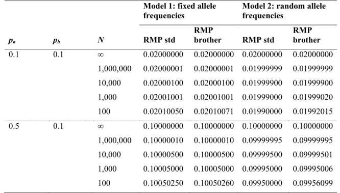
Table A1 provides examples of the values obtained for the RMP as calculated using standard HW

450

equations compared to those calculated using the approach described here (“RMP brother”). We

451

note that the “RMP brother” is generally equal to the standard RMP for a given set of parameters

452

N, pa and pb. The reader will note that the “RMP brother” tends to overestimate very slightly the 453

standard RMP, but the difference is negligible even for very small populations of interest. For

454

instance, in the worse case shown in Table A1 (i.e. under model 2, when N=100, pa=0.5 and 455

pb=0.1), “RMP brother”/“RMP std”= 1.000613 instead of 1. This is due to the effect of the 456

knowledge of the suspect’s genotype on the RMP for a finite population (which is a different

457

issue than the one addressed here). This effect is due to the negative covariance of genotypic

458

counts and increases with decreasing N. In other words, the observation of GS update our 459

knowledge of realized genotype frequencies in the population due to the constraint that allele

460

frequencies are either fixed (model 1) or random draw from a very large (infinite) population

461

having the postulated (reference) allele frequencies. Therefore, observing GS = a/b implies that 462

one of the 2Npa copies of allele a, and one of the 2Npb copies of allele b, in the population, are 463

found together in the suspect, meaning that other genotypes existing in the population must be

464

made from the remaining 2Npa -1 and 2Npb -1 copies, limiting possible values for genotype 465

counts in an increasing manner with decreasing N (independently of the suspect’s relatives issue).

466 467 468

Table A.1 Values obtained for the standard random match probability (“RMP std”) and the

469

random match probability accounting for the possibility that the brother is the random man

470

(“RMP brother”, which also includes the possibility for half sib), for a heterozygote a/b and

471

various settings of N, pa and pb (assuming =0). The standard RMP for model 2 integrates the 472

expected difference in the genotype frequencies in a finite population (2papb – papb /N) that is a 473

random draw from an infinite population (2papb) [25]. 474

Model 1: fixed allele

frequencies Model 2: random allele frequencies

pa pb N RMP std RMP brother RMP std RMP brother 0.1 0.1 ∞ 0.02000000 0.02000000 0.02000000 0.02000000 1,000,000 0.02000001 0.02000001 0.01999999 0.01999999 10,000 0.02000100 0.02000100 0.01999900 0.01999900 1,000 0.02001001 0.02001001 0.01999000 0.01999020 100 0.02010050 0.02010071 0.01990000 0.01992015 0.5 0.1 ∞ 0.10000000 0.10000000 0.10000000 0.10000000 1,000,000 0.10000010 0.10000010 0.09999995 0.09999995 10,000 0.10000500 0.10000500 0.09999500 0.09999501 1,000 0.10005000 0.10005000 0.09995000 0.09995006 100 0.10050250 0.10050260 0.09950000 0.09956099 475 476