Mono-hydrophone localization of baleen whales: a study of propagation using a spectral element method applied in Northern Chile

HAL Id: hal-02440437

https://hal.archives-ouvertes.fr/hal-02440437

Submitted on 15 Jan 2020

HAL is a multi-disciplinary open access

archive for the deposit and dissemination of

sci-entific research documents, whether they are

pub-lished or not. The documents may come from

teaching and research institutions in France or

abroad, or from public or private research centers.

L’archive ouverte pluridisciplinaire HAL, est

destinée au dépôt et à la diffusion de documents

scientifiques de niveau recherche, publiés ou non,

émanant des établissements d’enseignement et de

recherche français ou étrangers, des laboratoires

publics ou privés.

Mono-hydrophone localization of baleen whales: a study

of propagation using a spectral element method applied

in Northern Chile

Julie Patris, Dimitri Komatitsch, Maritza Sepúlveda, Macarena Santos, Hervé

Glotin, Franck Malige, Susannah Buchan, Mark Asch

To cite this version:

Julie Patris, Dimitri Komatitsch, Maritza Sepúlveda, Macarena Santos, Hervé Glotin, et

al..

Mono-hydrophone localization of baleen whales:

a study of propagation using a

spec-tral element method applied in Northern Chile.

Oceans 2019, Jun 2019, Marseille, France.

Mono-hydrophone localization of baleen whales: a

study of propagation using a spectral element

method applied in Northern Chile

Julie Patris

Universit´e d’Aix Marseille, Universit´e de Toulon,

CNRS, LIS

Marseille, France [email protected]

Dimitri Komatitsch

Centrale Marseille, CNRS, LMA Marseille, France

Maritza Sep´ulveda

Macarena Santos

Santiago, Chile

Herv´e Glotin

Universit´e de Toulon, CNRS, LIS

Toulon, France

Franck Malige

Universit´e de Toulon, CNRS, LIS

Toulon, France

Susannah Buchan

Universidad de Concepci´on Concepci´on, Chile

Mark Asch

Abstract—In the context of passive acoustic monitoring of large whales, we propose a new method for localizing blue whales (Balaenoptera musculus) from the acoustic recordings of only one sensor. We use a precise modelling of the sound propagation thanks to SPECFEM, a spectral element code for solving wave propagation equations. Based on field measurements in Northern Chile, we ran a simulation on a large supercomputer. We also exploited a recording device, Bombyx II, for one and a half months, with visual monitoring of the zone by a group of experts. We find that the method applied to the south east Pacific song of blue whales gives theoretical results of about 50% success in position recovery. Since we have redundancy in our data, we were able to locate the whale with a precision of 500 m over a box of 10 km by 5 km in the case when we have both visual detection and a strong acoustic signal. More tests should be performed before validating this method, but these first results are encouraging.

Index Terms—bioacoustics, acoustic propagation, underwater acoustics, source localization

I. INTRODUCTION

The conservation of cetaceans has been a major environ-mental concern for the last 50 years. The population of most large whales probably went down to the verge of extinction during the XXth century (Handbook of the mammals of the world, vol. 4 [1]), due to non sustainable whaling. Since then, new dangers are arising for large and small cetaceans, such as the general level of man-made noise in the oceans (see Boyd et al. 2011 [2], for an international quiet ocean experiment).

One of the first and the most difficult tasks for cetacean preservation is to estimate their actual number (see for instance Branch et al. 2004 [3] for the difficulty of estimating whale populations).

In this context, passive acoustic monitoring has been in-creasingly used to estimate cetacean populations (Mc Donald

and Fox 1999 [4]), although it is still a challenging technique for most species. Among other difficulties, estimating popu-lation numbers usually requires evaluating the distance of the emitter (see distance sampling methods, Marques et al. 2013 [5]) . This is usually done with an array of hydrophones, by the computation of time delays of arrival (Giraudet et al. 2008 [6]) or matched-field processing (Kuperman et al. 2004 [7]). However, installing an array of hydrophones means complicated field work that is not always possible. Although it is rather common to measure with towed hydrophones, for small cetaceans for instance (see Andriolo 2018 [8]), it remains difficult for fixed instruments and large wavelength measurements.

Several authors have proposed methods for mono-hydrophone localization, as early as in 1987 (Li and Clay [9]). Most of these works concern theoretical studies coupled with active experiments (Lee 1998 [10], Kuperman et al. 2001 [11], Le Touz´e et al. 2008 [12]) on short, broadband, known sounds (typically gunshots). Some studies also permit the recovery of a whale’s position or range based on short signals with multiple arrivals, such as the works of Mc Donald et al. 1999 [4] with fin whales (Balaenoptera physalus), Tiemann et al. 2006 [13] for sperm whales (Physeter macrocephalus) and Bonnel et al. 2014 [14] for bowhead whales (Balaena

mysticetus). One very interesting attempt is proposed by Harris et al. 2013 [15] and Matias et al. 2015 [16]. In their study they use seismic accelerometers where the 3-component signal recorded by the accelerometer allows to find the range (distance from sensor) of the emitting baleen whale up to 3 km more or less. What is more, numerous studies have shown that ‘naive’ methods based on sound intensity are very tricky and usually not reliable. For instance, Stimpert et al. 2015 [17]

compare the intensity of the received signal on a hydrophone on a tagged whale. The received level is not significantly different between the tagged whale and its neighbours.

To our knowledge, no attempt has been made towards recovering the position of the source for a long harmonic signal. Blue whales (Balaenoptera musculus) emit such long and complicated signals at very low frequency (see McDonald et al. 2006 [18]) with different patterns depending on the geographical zone. These songs also are remarkably auto-similar, with no perceptible difference between calls emitted by different individuals on intermediate time scales (see Ma-lige et al. 2019, [19]). An interesting case is the Chilean’ blue whale, with a song recently characterized by Buchan et al. in 2014 [20], presenting a high degree of complexity and regularity, and with animals repeatedly seen close to the shore in southern and northern Chile (Toro et al. [21]).

In this paper, we build a highly precise model of the sound propagation with spectral element methods (section II). This allows us to take advantage of the breaking of symmetry due to complex coastal environments and retrieve in 50% of the cases an approximate position of the emitter in laboratory tests (section IV). We also describe a field experiment conducted to test our method on blue whales’ songs (section III) and its results (section IV).

II. COMPUTATIONAL METHOD

A. General description

A fixed hydrophone is a common tool for oceanographers and biologists studying whales: it is not expensive, and it allows long term surveys of acoustical signals (see for instance Martinelli et al. 2016 [22] in Latin America). As stressed by Martinelli, such hydrophones have been used by many authors throughout the world to explore the presence of cetaceans, or study the patterns of emission of songs, or the characteristics of these songs.

However, it is very difficult now to recover the emitter’s position with only one hydrophone, especially for long calls. Thus, the amount of historical data recorded with a single fixed hydrophone cannot be used for the estimation of population density.

To achieve monohydrophone localization of long, low fre-quency signals, we propose using highly precise computational methods such as finite elements. These simulation techniques are time consuming but very precise, adapted both to transitory and harmonic signals. Time domain simulation allows us to work on an imput signal that is closer to a phenomenon of reverberation than simple separable echos.

B. Simulation techniques and software

Because sound is the primary method of communication in the ocean, the physics of sound propagation have been intensively studied, involving large scale simulation with var-ious methods (Jensen et al. 2011 [23]). Most of the efforts however have been focused on modelling active acoustics, which implies sending an artificial signal and analyzing its propagation through water and (or) ground (oil industry

prospecting, fisheries or military sonars). The most frequently used methods include ray propagation and parabolic methods (Etter 2012 [24]). Also, most methods assume the source of the sound to be a standard signal (a Gaussian or it’s derivative usually). In our case, the entry signal will be a complex biological signal.

Since we need high precision on the modelled form of the signal, we first need to develop fast and accurate computational methods for wave propagation problems based on state-of-the-art techniques such as the finite element method (FEM). This method presents a high degree of accuracy but requires large computing resources.

The method that we use for this study is SPECFEM open-source software (Tromp et al. 2008 [25]). SPECFEM was first developed for the simulation of seismic wave propagation at large scales in full wave forms. The method combines finite element methods and spectral elements, using a weak formulation of the equation of propagation, which is solved on a mesh of hexahedral elements (Komatitsch et al. 2005 [26]). The software and user manual can be found at the following web site: https://geodynamics.org/cig/software/specfem3d/.

The software accepts as an entry both the environment box and the signal to be propagated. The box is a 3D domain meshed with hexahedral elements. A mesher is included in the SPECFEM package so a meshing of the geographical environment can be performed by the software with infor-mation of the properties of the medium. In our case, the meshed domain is implemented mainly with information of a bathymetry, expressed as the coordinates of the interface between two media (ocean floor and water).

As a very accurate software, SPECFEM is however very time-consuming. Computational time for a single simulation depends mainly on the size of the box in terms of wavelengths. Traditionally, these tools are used in boxes up to around 100 wavelengths. Because both the sampling distance and time step depend on the frequency, the total computing time is highly dependent on the frequency and for the 3D version of SPECFEM, we usually have a dependency on the power of four (meaning that an augmentation of 20% of the frequency implies a doubling of the computing time). As a consequence, this modelling method can only be acceptable for either low frequencies or small boxes. Hence our idea of applying them to large baleen whales sounds, since large mysticetes are among the loudest and lowest-frequency sound producers in the sea. We found that modelling the sound propagation in our box, which is 10 km wide in latitude and longitude, and 500 m deep, for frequencies up to 50 Hz, we need around 10 000 hours of computation time. As we see, parallel algorithms of computation are extremely important for such methods, and this is also one of the important achievements of the SPECFEM package.

One of the problems of this family of numerical methods is to model ‘open’ box frontiers. We used Stacey [27] absorbing conditions, proposed by the software. At the same time, with the help of Alexis Bottero and Vadim Monteiller at the LMA in Marseilles, we worked on the inclusion of a depth-dependant

sound velocity inside the water. This function was already present is the code, but incompatible with the internal mesher. It is now possible to use both in a simulation.

Our project involves not only the simulation of the wave propagation, but also an inverse problem to find the position where our simulated signal is closer to the measured one. Having an order of 10 000 hours for one simulation prohibits a classical inverse method, so we propose an original idea to solve our inverse problem with only one simulation. Our modelling is based on the reciprocity principle of the Green’s function (see for instance the book Computational Ocean Acousticsby Jensen et al. [23]), which is the acoustical expres-sion of the Helmholtz principle in optics (simply characterized by the general principle: if I can see you, you can see me). In a static, linear medium, the Helmholtz principle states that if one was able to swap the sensor and wave source, the measurement of flux would remain equal. Tests with SPECFEM simulations show that the differences between the two signals are less than numerical noise.

Instead of modelling the propagation from every given point of the box towards the hydrophone, we are thus going to model the propagation from the hydrophone towards the possible position of the whale. This is incomparably more efficient for our problem, since we will only have to execute one simulation and just look at the simulated signal at a number of points (which is easily done by adding ‘receiver’ points in SPECFEM).

C. Laboratory tests

Before ground-truthing our method, we performed a series of ‘laboratory tests’. These tests are done by simulating the position of several randomly placed whales in our model and correlating the output to find the best grid position for each simulated whale.

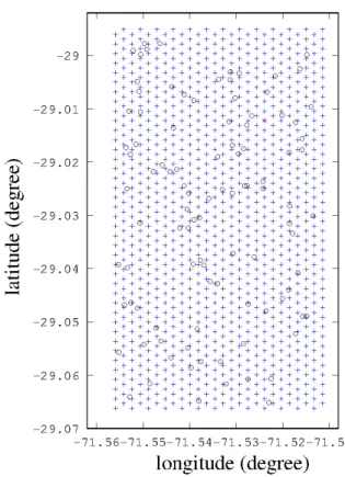
We thus constructed a three-dimensional grid of 4 ×1040 = 4260 _{points. This grid is used as the receiver positions in a} SPECFEM simulation, and as possible emitter positions in our test.

Figure 1 shows the aspect of the grid in a horizontal plane. The step between two consecutive points is 200 meters. Thus, it won’t be possible to retrieve the position of the whale at a precision higher than 100 meters, a very optimistic precision given our context. Our grid does not cover the entire domain of simulation: to prevent potential side effects at the frontier, we began our grid 1 km away from the borders of our simulation box. The grid has four layers in vertical position, with depths of 10, 25, 50 and 90 m. From the work of Oleson et al. 2007 [28], we expect our singing whales to be at a depth of 10 to 40 meters.

Added to these receivers, for our test we introduced 100 random points representing the ‘whales’. Thus, the signal ‘received’ by each of these ‘whales’ is considered in our test as the original measured signal, and will be correlated to the signals obtained on each point of the grid. The 100 simulated whales’ positions are random in longitude, latitude and depth, within our modelled box.

Fig. 1. 2D view of our simulation grid. Circles represent one hundred randomly placed ’whales’, i.e. positions from which a signal is emitted. Star is the hydrophone position.

The simulation was performed on the OCCIGEN su-percomputer of CINES (Centre Informatique National de l’Enseignement Sup´erieur), on 600 cores during 21 hours. We obtained 4260 files of propagated sound, on our grid of 1040 points and 4 horizontal layers (10m, 25m, 50 m and 90m), plus 100 randomly chosen ‘whale’ positions for the theoretical tests.

Each file is a waveform of 19.5 seconds total duration, with 650 000 steps of 0.00003 seconds. The simulation box has a size of 5.2 km by 8.7 km, for a total depth of 500 meters. The minimum length of a meshed element is 0.57 m, the maximum length is 17.3 m. With these parameters, the predicted maximum frequency admitted by the simulation is 69 Hz, which is remarkably high for a finite element modelling of this size.

We used an impulsion (‘Dirac peak’ truncated to the maxi-mum frequency) as the entrance signal in the time domain. Thus, we can convolve later on by an appropriate source function. This allows more freedom in the choice of a source, and we can apply the same simulation to different tests.

If this method is to be made available for biologists studying whale populations, it is important to notice that only one large simulation will be necessary for one location. After the simulation is completed, the inversion is done by correlating every resulting signal with the original one (in the case of

our test, with one of the ‘whales’ signals). This correlation does not need special computer resources. We performed the correlation for fifty examples in about 6 hours on a small personal computer.

To find which position is closer to our ‘test’ signal, we have to compare two signals. However, the comparison must not take into account the intensity of the signal, because, though the emitted songs are very similar in shape, they can differ a lot in intensity (see Stimpert et al. 2015 [17]). The comparison cannot be tuned on the time of arrival, because of course this data is not known in real conditions.

The correlation is computed through a little Octave [29] routine with two complementary methods:

• First, we compute the normalized correlation function

between our ‘whale’ signal (Sw) and each of the signals

corresponding to a point in the grid Si. Then, we find

the maximum of each of these correlation functions (MaxCori). MaxCori is a value affected to each point of

the grid, giving the information of how close the ‘whale’ signal is to the signal ‘emitted’ on this point. We can then transform this variable into a map which will be called the Maxima of Correlation functions map (MaxCor map). The maximum of this map gives the point where the whale is supposed to be (MaxCor best position).

• As a second method, we compute a correlation coefficient

FFTCori between the modulus of the Fourier transform

of the ‘whale’ signal and the modulus of the Fourier transform of each of our signals on the grid’s points. This variable is transformed into a map (FFTCor map). The maximum of this map gives the point where the whale is according to this method (FFTCor best position).

III. FIELD EXPERIMENT

In order to ground-truth our method, we set up a field experiment close to Cha˜naral Island Natural Reserve, 600 km North of Santiago de Chile. This field experiment comprises: - the mooring of a fixed hydrophone for one and a half months during the summer of 2017,

- a visual follow-up of the zone between the island and the shore,

- measures of physical and biological properties to run an adapted simulation.

A. Acoustic device

The hydrophone and recording package ’BOMBYX II’ was deployed at 15/20 meters below the surface on a mooring where water column depth was 70 meters-depth. It was set in the northern coast of Chile, 29◦00′44′′ _{south and 71}◦31′26′′

west, during the austral summer of 2016/2017, between the 16th of January 2017 and the 27th of February 2017. Data were collected during three periods of two weeks in January and February [30]. The hydrophone package ’BOMBYX II’ was mounted by the University of Toulon and comprises a Cetacean Research C57 hydrophone (very high sensibility, flat response down to 20 Hz, omnidirectional at low frequencies

and listening in a plane orthogonal to its axis in high frequen-cies), alimented by 9 V through a high-pass filter (C=47F, frequency cut 0.15 Hz) and a commercial SONY PCM-M10 recording device (gain 6, Rin = 22 kOhm) equipped with a 256 GB memory card, set up in a specialized tube made by Osean able to resist high pressure. Recording was done at a sample rate of 48 kHz and a dynamical range of 16 bits.

B. Visual follow-up

The visual observations were carried out by a team of experts that were posted for two 12-day long missions on the island of Cha˜naral, by special permit of the CONAF since the whole island is a protected area (Maritza Sepulveda and Macarena Santos were in charge of this part of the project, see Sepulveda et al. 2017 [31]). The team was equipped with two theodolites. From 9 am to 6 pm, when the wind was lower than 4 Beaufort, they looked for cetaceans in the channel between the island and the coast. During this period of time, and every hour, they scanned the whole area for animals and noted their positions and species.

The data collected in two rounds of 12 days of observation in 2017 is shown on figure 2. Observations are from the 17/01/2017 to the 28/01/2017 and from the 15/02/2017 to the 26/02/2017. Three species of large baleen whales are com-monly found around the Isla de Cha˜naral reserve: fin whales (Balaenoptera physalus), the most frequent, blue whales

(Bal-aenoptera musculus) and humpback whales (Megaptera

no-vaeangliae). This figure however does not reflect the number of animals in the zone, since the same animal can be marked several times.

Fig. 2. Large whales sighting from the island of Cha˜naral by the team of Sepulveda and Santos (see [31]). Star is the recording hydrophone, and squares mark the limit of the modelled box.

The area covered by visual scanning is more or less the same as the box used for modelling.

We are specifically interested in blue whales since their song is our chosen signal. However, the blue whales are not the most frequent marine mammals here. Approximately 40 out of 500 sightings concern blue whales, spotted on 9 different days.

Some animals have been spotted during the whole day (for instance, the first detection of a blue whale on the 18/01/2017 was annotated 17 times during the whole day), others have been seen only once.

What’s more, all blue whales do not produce songs: ac-cording to Oleson et al. 2007 [28] only males emit this type of vocalization. These vocalizations are thus supposed to be linked to sexual display and play a role in reproduction. The Humboldt archipelago zone, to which the channel belongs, is confirmed as a feeding zone for the large rorquals (see for instance Toro et al. 2016 [21]) . However, the continuous recording of blue whale songs in our experiment (see Buchan et al. 2019, in prep. [32]) as in other feeding zones seem to show that blue whales emit songs even in feeding grounds, though maybe not as frequently as in other types of habitats.

C. Physical and biological parameters of the model

a) Bathymetry: Official maps proving to be highly im-precise for our zone of interest, we measured a few hundred depths with a simple echo sounder during several campaigns in 2016, 2017 and 2018. We joined our measures to those of the technical base-line report of Gayer 2008 [33] and interpolated a bathymetry surface of a zone including our modelled box.

b) Sound profile: For the variation of the velocity of sound in water, we used both base-line information on tem-perature and salinity from Gayer 2008 [33] and our own opportunistic measurements of temperature, performed each time the recording device was changed for maintenance and during diving campaigns in the same geographical zone. The summary of this data leads to two averaged curves, one for winter and one for summer. Only the summer profile, show in figure 3 was used in our simulation since recording was done in summer. -350 -300 -250 -200 -150 -100 -50 0 1496 1498 1500 1502 1504 1506 1508 1510 Depth (m) Sound velocity (m/s) Chanaral Summer

Fig. 3. Sound profile in Cha˜naral (data computed from Gayer’s report, 2008 [33] and our own measurements).

c) Ground properties: The ground properties were set consulting Gayer’s report, 2008 [33] and information from local fishermen, showing that most of the canal between the

island and the shore is covered with sand and sediments. Of course, this is a rather crude estimation since the uneven bathymetry is probably due to some rocky surfaces and as-perities. However, we could not measure details of the ground properties, so we checked that our simulations were relatively robust to a change in the value of the ground sound velocity and density. It is worth noting, however, that the simulation leads to very different results if we imagine a purely rocky ground (hard suface), inducing strong echos (probably Scholte waves due to shear waves velocity in a solid) that are not seen in our data. Thus we chose to caracterize our ground layer as a fluid sediment with a sound velocity of 1650 m/s and a density of 1800 kg/m3

.

d) Source signal: The source signal issue was addressed in detail after the simulation was done. The blue whale song is a very stable signal. However, the source signal serving as an input to our simulation has to be an ‘emitted’ signal, whereas we of course only have ‘received’ signals (signals received after an unknown process of propagation). Three methods of constructing a source signal were explored, they are described in our research report ‘Reflexions sur le signal source’ (LIS, Santiago, April 2018 [34]). Basically, one is obtained through a mathematical model (hereafter called mod), another through a time reversal inversion method (hereafter called inv) and the last one performing an average over several recorded signals (moy). For each of these three methods, we convolved the input signal with the impulse response of the propagation model on the 4160 points of the grid.

Fig. 4. Input signal for the simulation in time domain. Upper left: example of received signal. Upper right: signal reconstructed from a time reversal method (inv). Lower left: signal modelled with a mathematical function (mod). Lower right: signal averaged over five examples of received signals (moy).

D. Choice of the set of data

The blue whale recordings found in the first year of record-ing are described in Buchan et al. 2019 ( [32], in prep.). More than 2000 song units have been detected by a visual inspection,

meaning song detections almost every day for this period of time.

However, the signal to noise ratio of these detections is highly variable. Blue whales are known to be among the strongest sources of biological sound: a song intensity can be measured up to 180 dB ref 1 µPa at 1 m (Samaran et al. 2010 [35]). They are also very low frequency sounds (usually between 15 Hz and 100 Hz, McDonald et al. 2006 [18]), propagating in a very efficient manner in the ocean. It is probable that we can perceive sounds emitted by a very far away animal, the detection range reaching 100 km in known experiments (Dreo et al. 2018 [36]).

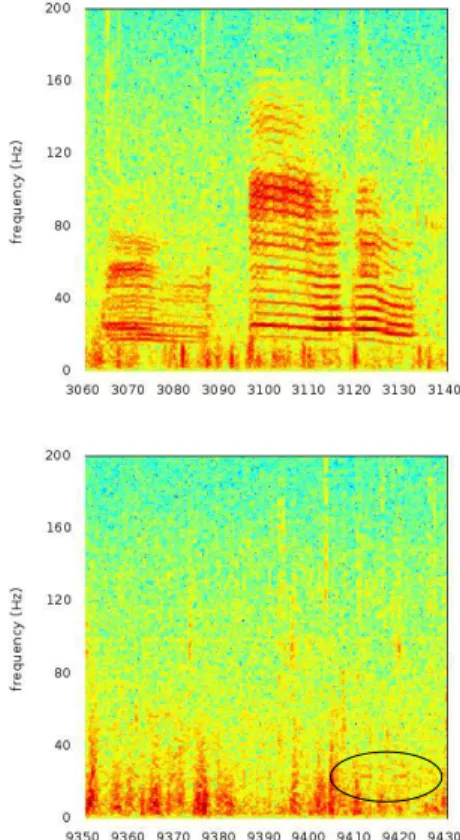
The detections we obtain in our data, range from a very high signal-to-noise ratio to very faint signals. Figure 5 shows the difference of time/frequency representation of two detections.

Fig. 5. Time-frequency representation of two blue whale’s song detections. Top: extract from a recording on February, 2nd

2017 with high signal to noise ratio, every detail of the song appears. Bottom: extract from a recording on February, the 11th

2017, low signal to noise ratio, only the louder part of the song, two 23-Hz tonal sounds, around 5 s long are visible in the representation. Both images are 80 s-long extracts, and FFT was computed on Hanning windows of 212points.

As shown in section , our method is sensitive to the richness of the input signal. Thus, a very faint signal such as the one represented in the right part of the figure 5 is not a good candidate for our method. What’s more, it is probable that such a faint signal comes from a distant animal. Indeed, though signal intensity is not a good indicator of source distance, in this case, where these songs are remarkable for their stability, we can infer that such a drastic change in signal to noise ratio

(around 30 dB of difference in SNR) is at least partly an effect of distance or masking. Thus, there is very little probability that the whale was present in our modelled box when emitting this signal.

We cannot expect a matching ratio better than 50% of the signals, as this is what we have with a ‘perfect’ modelling, that is the theoretical tests explained in the previous section. Thus, we need a redundancy of data to ascertain the position of the whale. Since Isla de Cha˜naral reserve is a feeding ground, the whales usually do not move much, doing slow loops around the food source. Fortunately, the song of a blue whale is usually the repetition (for hours) of the same unit, repeated every 2 minutes. We thus have long series of signals in our data, probably emitted by the same individual.

To test our method of localizing animals in a 10 km wide box, we will thus need to select series of high signal-to-noise ratio songs. These are not so frequent in our recording, matching the rather scarce visual detection from the island.

Selecting detections with a series of at least 10 song’s units with signal-to-noise ratio better than 25 dB, we found the following useful data:

• recording of the 19/01/2017: 16 units, spanning 1 hour,

in the night, rather low signal to noise ratio (set 1);

• recording of the 24/01/2017: 21 units, spanning 1 hour

in the morning (set 2);

• recording of the 24/01/2017: 20 units, spanning 2 hours

in the afternoon, rather low signal to noise ratios (set 3);

• recording of the 02/02/2017: 52 units with very high

signal-to-noise ratio, spanning 3 hours during the night (set 4);

• recording of the 22/02/2017: 16 units with loud signal

but also a lot of noise, spanning 1 hour during the night (set 5);

IV. RESULTS AND DISCUSSION

A. Results of the laboratory tests

As described in section II, a first way of testing our method is through 100 simulated whales. These are randomly chosen positions, that we try to recover by correlating the received signal with all received signals in the grid. This test does not allow a check of the consistency between the model’s physical and biological parameters and the ground reality. However, it shows the possibilities of the inversion method for the specific bathymetry and source signal. In each test, we tried two different correlation methods: one correlates the waveforms (MaxCor), the other the spectra (FFTCor); and three methods for constructing the source signal described in section II: modelled source (mod), signal from an inversion process (inv) and source averaged over several received signals (moy).

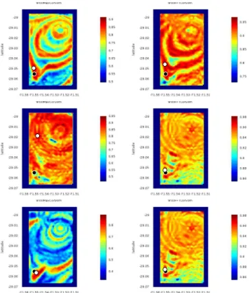
Some correlation maps in 2D, showing only the chosen depth layer, are shown in figure 6. In this example we see a good match for 4 maps out of 6: the two upper maps are from a wrong layer, which coincides with a bad guess in horizontal position.

Fig. 6. Correlation maps from Cha˜naral simulation: example of the 100th simulated whale, situated at 64 m depth. On each map, the real position is marked with a black dot and the one recovered by the method is marked by a white dot. From top to bottom: mod, inv and moy methods for the sources. Left column: method of temporal correlation (MaxCor), right column: method of frequency-domain correlation (FFTCor). All maps are on the 50 m layer, except the MaxCor methods with sources inv (first column, second row) which is 10 m layer and moy (first column, third row) which is 90 m layer).

General results are presented in table I.

TABLE I

RESULTS FOR LABORATORY TESTS. EACH TEST WAS PERFORMED OVER

100 ‘SIMULATED’WHALES PLACED RANDOMLY. TWO CORRELATION

METHODS AND THREE TYPES OF SOURCE SIGNAL ARE COMPARED. .

Simulation results Method for the source

mod inv moy

found at less than 200m MaxCor 34 36 43

FFTCor 19 24 32

found at less than 500m MaxCor 50 60 62

FFTCor 32 45 43

range at less than 500m MaxCor 78 87 86

FFTCor 57 68 71

depth MaxCor 79 68 91

FFTCor 70 66 71

On average over all methods, the whale’s position is re-covered in 50% of the cases and the range in 75%, with a precision of 500 meters. These are not very high numbers, especially considering this is a test with simulated whales, so that the quality of our physical and biological model is not tested. Thus, a redundancy of data will be necessary: one cannot expect to find the position of a whale without several signals being used. Another remark is that range is

easier to recover than position (which is range plus azimuth). This is to be expected since the main symmetry of shallow water is cylindrical around the vertical line passing through the sensor. It is interesting to note, however, because range is often sufficient for statistical purposes (density estimation).

Overall, for all tests, the correlation in waveform gives better results, probably because it includes more information (the phase information is preserved, whereas in the FFTCor method we use only the modulus of the FFT).

There are significant differences between the three methods for the source that we tested, which is surprising if we consider that for this simulated test, strictly the same source is used for the pseudo-received and the simulated signals. The first of the three methods, the one using a mathematical source, is clearly less efficient than the other two, directly derived from observed signals. The probable cause is the richness of a real signal as compared with a mathematical one. Thus, it is important to have a lot of information in the input signal, so as to see the effect of propagation better.

B. Field experiment results

When we cross the visual observation results with the high signal to noise selected acoustic songs, we find only one intersection. This is the only one of our 5 testing sets of data that was recorded in day time, on January 24th, 2017. Thus, this is the only example where we have a very strong acoustic recording and a visual detection at the same moment.

For this set of data, we then correlated the received signal with the 4160 points of our grid, for each of the 3 methods. We also did the same for the other sets of data, even though we do not have a visual match for them.

For each unit, a ‘best’ position is computed. Then, we cut our horizontal box in 78 rectangles of approximately 0.5 by 0.4 nautical miles. We then counted the number of positions found in each of these rectangles. Thus, we constructed a coarse ‘probability of presence’, or density map.

Both the mathematical modelling method (mod) and the average method (moy) lead to incoherent results: either the density is uniformly distributed, or the results point to an impossible place (below the ground). The correlation in the time domain does not give results either.

In the case of the source obtained by the inversion method (inv), however, and for the frequency domain correlation, we find that in 3 out of the 5 sets, the density map shows a plausible maximum. The two sets that do not present a plausible result are the sets with the lowest signal-to-noise ratio.

We show in figure 7 the three maps corresponding to plausible results. These are the set 2 (January, the 24th), 4 (February, the 2nd) and 5 (February, the 22nd). For the set 2, we have a visual confirmation of the position, and this corresponds to the position found. For the two other sets, we find the animal close to a rocky peninsula. Interestingly, a citizen science project led by the national park service CONAF found two blue whales in this zone on the morning of Feb, 2nd

zone (Susannah Buchan and Marinella Maldonado, private communication).

Fig. 7. Density maps for three of our data sets. Left: set 2,(January, the 24th ), middle: set 4 (February, the 2nd

) right: set 5 (February, the 22nd ).

C. Discussion

In this section we comment on the possible interpretation of these results and on future works.

Let’s consider first the reason why only one source gave plausible results. The mathematical model (mod) did show a poor efficiency in the theoretical tests. It seems probable that this model is not rich enough in harmonics, basically, that it is not similar enough to a biological signal. The averaged source did not work either: when we examine this source, we see that though the first part of the unit is well reproduced, thanks to the very high stability in frequency of the songs, the second part is not well reproduced. This is due to the fact that the phase difference between the first tonal sound and the second one (slightly lower in frequency) is not randomly distributed in different songs. Thus, the averaging reduces the second part (see figure 4). The poor efficiency of the time domain correlation method (MaxCor) compared to the frequency domain (FFTCor) can be explained by the same phenomenon: the correlation in time domain is efficient for the first part, but the slight shift between the first and second part of the song blurs the correlation in this second part. For the theoretical test, this was not a problem since the signal was correlated with a source that has the same phase difference, thus explaining the good results in theoretical tests of the time domain correlation.

The last method, with the source obtained by inversion (inv), gives interesting results. The only case were we have a visual identification is recovered correctly. Two other cases show animals close to a zone where a lot of animals have been seen in the morning, before the tourists boats are out (personal observation, communication from residents). The two cases without plausible results can be interpreted as concerning animals that were out of the model box, since the signal-to-noise ratios were low in both cases.

The most obvious conclusion of this study is that one encouraging result has been found, but a lot more has to be done before validating the method. More data is needed, but this is a very long and difficult prospect, since coupled visual and acoustic data are not very frequent. However, this method could be adapted with comparatively little effort to another coastal place and other types of signals, opening various possibilities.

ACKNOWLEDGMENT

This work was written in memory of Dimitri, who left us just before the end of our common study. We stay with his wonderful tool SPECFEM and the memory of his energy, eternal goodwill and deep competence that helped us to go on. Thanks to Paul Cristini for discussions on acoustics, to Vadim Monteiller for technical support and especially to Alexis Bottero for hours of working on SPECFEM together... Many thanks to all the friends in ’la caleta’, and especially Cesar Villaroel and everyone at the ExploraSub diving cen-ter, and Marinella Maldonado and her colleagues from the CONAF. We acknowledge the help of STIC-Am Sud funding via the project BRILAM 17-STIC-01. Partly funded by FUI 22 Abyssound, ANR-18-CE40-0014 SMILES, and ANR-17-MRS5-0023 NanoSpike. We thank SABIOD.org, and EADM MADICS CNRS scaled bioacoustic groups for their support.

REFERENCES

[1] D. Wilson and R. Mittermeier, Eds., Handbook of the mammals of the

world. Lynx Edicions, 2014, vol. 4.

[2] I. L. Boyd, G. Frisk, E. Urban, P. Tyack, J. Ausubel, S. Seeyave, D. Cato, B. Southall, M. Weise, R. Andrew, T. Akamatsu, R. Dekeling, C. Erbe, D. Farmer, R. Gentry, T. Gross, A. Hawkins, F. Li, K. Metcalf, J. Miller, D. Moretti, C. Rodrigo, and T. Shinke, “An international quiet ocean experiment,” Oceanography, vol. 24, no. 2, p. 174181, 2011. [3] T. A. Branch, K. Matsuoka, and T. Miyashita, “Evidence for increases

in antarctic blue whales based on bayesian modelling,” Marine Mammal

Science, vol. 20, no. 4, pp. 726–754, 2004.

[4] M. McDonald and C. Fox, “Passive acoustic methods applied to fin whale population density estimation,” J. Acoust. Soc. Am., vol. 105, no. 5, pp. 2643–2651, May 1999.

[5] T. A. Marques, L. Thomas, S. W. Martin, D. K. Mellinger, J. A. Ward, D. J. Moretti, D. Harris, and P. L. Tyack, “Estimating animal population density using passive acoustics,” Biol. Rev., vol. 88, pp. 287–309, 2013. [6] P. Giraudet and H. Glotin, “Real-time 3d tracking of whales by echo-robust precise tdoa estimates with a widely-spaced hydrophone array,”

Applied Acoustics, vol. 67, no. 11, pp. 1106–1117, 2008.

[7] W. A. Kuperman and J. F. Lynch, “Shallow-water acoustics,” Physics

Today, pp. 55–61, october 2004.

[8] A. Andriolo, F. R. de Castro, T. Amorim, G. Miranda, J. D. Tullio, J. Moron, B. Ribeiro, G. Ramos, and R. R. Mendes, Advances in Marine

Vertebrate Research in Latin America. Springer International Publishing AG 2018, 2018, ch. Marine Mammal Bioacustics Using Towed Array Systems in the Western South Atlantic Ocean, pp. 113–147.

[9] S. Li and C. Clay, “Optimum time domain signal transmission and source location in a waveguide: Experiments in an ideal wedge waveg-uide,” J. Acoust. Soc. Am., vol. 82, no. 4, pp. 1409–1417, 1987. [10] Y. P. Lee, “Time-domain single hydrophone localization in a real shallow

water environment,” IEEE, pp. 1074–1077, 1998.

[11] W. A. Kuperman, G. L. DSpain, and K. D. Heaney, “Long range source localization from single hydrophone spectrograms,” J. Acoust. Soc. Am., vol. 109, no. 5, pp. 1935–1943, 2001.

[12] G. L. Touz´e, J. Torras, B. Nicolas, and J. Mars, “Source localization on a single hydrophone,” IEEE Journal of Oceanic Engineering, vol. 25, no. 3, pp. 337–343, 2000.

[13] C. O. Tiemann, A. M. Thode, J. Straley, V. OConnell, and K. Folk-ert, “Three-dimensional localization of sperm whales using a single hydrophone,” J. Acoust. Soc. Am., vol. 120, no. 4, pp. 2355–2365, 2006. [14] J. Bonnel, A. M. Thode, S. B. Blackwell, K. Kim, and A. M. Macrander, “Range estimation of bowhead whale (balaena mysticetus) calls in the arctic using a single hydrophone,” J. Acoust. Soc. Am., vol. 136, no. 1, pp. 145–155, 2014.

[15] D. Harris, L. Matias, L. Thomas, J. Harwood, and W. H. Geisser, “Applying distance sampling to fin whale calls recorded by single seismic instruments in the northeast atlantic,” J. Acoust. Soc. Am., vol. 134, no. 5, pp. 3522 – 3535, 2013.

[16] L. Matias and D. Harris, “A single-station method for the detection, classification and location of fin whale calls using ocean-bottom seismic stations,” J. Acoust. Soc. Am. 138 (1), vol. 138, pp. 504–520, 2015. [17] A. K. Stimpert, S. L. DeRuiter, E. A. Falcone, J. Joseph, A. B. Douglas,

and D. J. More, “Sound production and associated behavior of tagged fin whales (balaenoptera physalus) in the southern california bight,” Anim

Biotelemetry (2015) 3:23, vol. 3, no. 23, 2015.

[18] M. McDonald, S. L. Mesnik, and J. A. Hildebrand, “Biogeographic characterisation of blue whale song worldwide: using song to identify populations,” J. Cetacean Res. Manage., 2006.

[19] F. Malige, J. Patris, S. J. Buchan, K. M. Stafford, L. E. Rendell, F. W. Shabangu, K. P. Findlay, R. Hucke-Gaete, S. Neira, C. W. Clark, , and H. Glotin, “Joint analysis of year decline in pulsation and peak frequency of the sep2 blue whale song type with the help of a new mathematical model of pulsated sound,” unpublished submitted to J. Acoust. Soc. Am., 2019.

[20] S. Buchan, R. Hucke-Gaete, L. Rendell, and K. Stafford, “A new song recorded from blue whales in the corcovado gulf, southern chile, and an acoustic link to the eastern tropical pacific,” Endang Species Res, vol. 23, pp. 241–252, 2014.

[21] F. Toro, Y. A. Vilina, J. J. Capella, and J. Gibbons, “Novel coastal feeding area for eastern south pacific fin whales (balaenoptera physalus) in mid-latitude humboldt current waters off chile,” Aquatic Mammals, vol. 42, no. 1, pp. 47–55, 2016.

[22] A. Martinelli, M. Nery, and J. Torres-Florez, “Forty four years of using bioacoustics to study aquatic mammals in latin america : state of the art of a growing research area,” in 2nd Listening for Aquatic Mammals in

Latin America Workshop (LAMLA 2), Valparaso, Chile, 2016. [23] F. B. Jensen, W. A. Kuperman, M. B. Porter, and H. Schmid,

Com-putational Ocean Acoustics, 2nd ed., W. W.Hartmann, Ed. Springer, 2011.

[24] P. C. Etter, “Advanced applications for underwater acoustic modeling,”

Advances in Acoustics and Vibration, 2012.

[25] J. Tromp, D. Komatitsch, and Q. Liu, “Spectral-element and adjoint methods in seismology,” Communication in Computational Physics, vol. 3, no. 1, pp. 1–32, 2008.

[26] D. Komatitsch, S. Tsuboi, and J. Tromp, “The spectral-element method in seismology,” in Seismic Earth: Array Analysis of Broadband

Seismo-grams, ser. Geophysical Monograph, A. Levander and G. Nolet, Eds. American Geophysical Union, 2005, vol. 157, pp. 205–228.

[27] R. Stacey, “Improved transparent boundary formulations for the elastic-wave equation,” B.S.S.A, vol. 78, pp. 2089–2097, 1988.

[28] E. M. Oleson, J. Calambokidis, W. C. Burgess, M. A. McDonald, C. A. LeDuc, and J. A. Hildebrand, “Behavioral context of call production by eastern north pacific blue whales,” Mar Ecol Prog Ser, vol. 330, pp. 269–284, 2007.

[29] J. W. Eaton, D. Bateman, and S. Hauberg, GNU Octave version 3.0.1

manual: a high-level interactive language for numerical computations. CreateSpace Independent Publishing Platform, 2009, ISBN 1441413006. [Online]. Available: http://www.gnu.org/software/octave/doc/interpreter [30] J. Patris, F. Malige, and H. Glotin, “Construction et mise en place d’un

systme fixe d’enregistrement large bande pour les c´etac´es “bombyx 2” isla de chaaral, ´et´e austral 2017,” LSIS CNRS, Tech. Rep. 2017-03, march 2017.

[31] M. Sep´ulveda, M. Santos, and G. Pavez, Whale-watching en la reserva

marina Isla Cha˜naral : manejo y planificaci´on para una actividad sustentable. Universidad de Valpara´ıso, 2017.

[32] S. Buchan, J. Patris, F. Malige, N. Balcazar-Cabrera, G. Alosilla, and H. Glotin, “Southeast pacific blue whale song recorded off isla chaaral, northern chile,” unpublished, 2019.

[33] C. Gayer, “Evaluacin de lnea base de las reservas marinas ”isla chaaral” e ” isla choros-damas”,” Universidad Catlica del Norte, Coquimbo, Tech. Rep., 2008.

[34] J. Patris, F. Malige, and H. Glotin, “Reflexions sur le signal source,” LSIS CNRS, Tech. Rep. 2018-04, april 2018.

[35] F. Samaran, C. Guinet, O. Adam, J.-F. Motsch, and Y. Cansi, “Source level estimation of two blue whale subspecies in southwestern indian ocean,” J. Acoust. Soc. Am., vol. 127, no. 6, pp. 3800–3808, 2010. [36] R. Dreo, L. Bouffaut, E. Leroy, G. Barruol, and F. Samaran, “Baleen

whale distribution and seasonal occurrence revealed by an ocean bottom seismometer network in the western indian ocean,” Deep Sea Research