HAL Id: hal-03047191
https://hal.archives-ouvertes.fr/hal-03047191
Submitted on 16 Dec 2020
HAL is a multi-disciplinary open access
archive for the deposit and dissemination of
sci-entific research documents, whether they are
pub-lished or not. The documents may come from
teaching and research institutions in France or
L’archive ouverte pluridisciplinaire HAL, est
destinée au dépôt et à la diffusion de documents
scientifiques de niveau recherche, publiés ou non,
émanant des établissements d’enseignement et de
recherche français ou étrangers, des laboratoires
Span-core Decomposition for Temporal Networks:
Algorithms and Applications
Edoardo Galimberti, Martino Ciaperoni, Alain Barrat, Francesco Bonchi, Ciro
Cattuto, Francesco Gullo
To cite this version:
Edoardo Galimberti, Martino Ciaperoni, Alain Barrat, Francesco Bonchi, Ciro Cattuto, et al..
Span-core Decomposition for Temporal Networks: Algorithms and Applications. ACM Transactions on
Knowledge Discovery from Data (TKDD), ACM, 2020, 15 (1), pp.1-44. �10.1145/3418226�.
�hal-03047191�
Span-core Decomposition for Temporal Networks:
Algorithms and Applications
Edoardo Galimberti, Martino Ciaperoni, Alain Barrat,
Francesco Bonchi, Ciro Cattuto, Francesco Gullo
December 16, 2020
Abstract
When analyzing temporal networks, a fundamental task is the iden-tification of dense structures (i.e., groups of vertices that exhibit a large number of links), together with their temporal span (i.e., the period of time for which the high density holds). In this paper we tackle this task by introducing a notion of temporal core decomposition where each core is associated with two quantities, its coreness, which quantifies how densely it is connected, and its span, which is a temporal interval: we call such cores span-cores.
For a temporal network defined on a discrete temporal domain T , the total number of time intervals included in T is quadratic in |T |, so that the total number of span-cores is potentially quadratic in |T | as well. Our first main contribution is an algorithm that, by exploiting contain-ment properties among span-cores, computes all the span-cores efficiently. Then, we focus on the problem of finding only the maximal span-cores, i.e., span-cores that are not dominated by any other span-core by both their coreness property and their span. We devise a very efficient algo-rithm that exploits theoretical findings on the maximality condition to directly extract the maximal ones without computing all span-cores.
Finally, as a third contribution, we introduce the problem of temporal community search, where a set of query vertices is given as input, and the goal is to find a set of densely-connected subgraphs containing the query vertices and covering the whole underlying temporal domain T . We derive a connection between this problem and the problem of finding (maximal) span-cores. Based on this connection, we show how temporal community search can be solved in polynomial-time via dynamic programming, and how the maximal span-cores can be profitably exploited to significantly speed-up the basic algorithm.
We provide an extensive experimentation on several real-world tem-poral networks of widely different origins and characteristics. Our results confirm the efficiency and scalability of the proposed methods. More-over, we showcase our techniques in a number of applications on temporal networks describing human face-to-face interactions in various settings. Our main findings in this regard highlight the relevance of the notions
of (maximal) span-core and temporal community search in analyzing so-cial dynamics, detecting/correcting anomalies in the data, and graph-embedding-based network classification.
1
Introduction
A temporal network1 is a representation of entities (vertices), their relations (links), and how these relations are established/broken over time. Notice that here we will consider discrete times, i.e., the temporal networks can be repre-sented as a time-ordered series of snapshots (instantaneous graphs). Extracting dense structures (i.e., groups of vertices exhibiting a large number of links with each other), together with their temporal span (i.e., the period of time for which the high density is observed) is a key mining primitive to characterize such tem-poral networks and extract relevant structures. This type of pattern enables fine-grain analysis of the network dynamics and can be a building block towards more complex tasks and applications, such as finding temporally recurring sub-graphs or anomalously dense ones. For instance, they can help in studying contact networks among individuals to quantify the transmission opportunities of respiratory infections in a population and uncover situations where the risk of transmission is higher, with the goal of designing mitigation strategies [38]. Anomalously dense temporal patterns among entities in a co-occurrence graph (e.g., extracted from the Twitter stream) have also been used to identify events and buzzing stories in real time [5, 15]. Another example concerns scientific col-laboration and citation networks, where these patterns can help understand the dynamics of collaboration in successful professional teams, study the evolution of scientific topics, and detect emerging technologies [28].
In this paper we adopt as a measure of density of a pattern the minimum degree holding among the vertices in the subgraph during the pattern’s span. The problem of extracting all these patterns is tackled by introducing a notion of temporal core decomposition in which each core is associated with its span, i.e., an interval of contiguous timestamps, for which the coreness property holds. We term such a notion of temporal core span-core.
Moreover, in several application scenarios it is typically required to identify only those dense patterns that contain a given set of query vertices. We therefore introduce the problem of temporal community search, whose goal is to find a set of cohesive temporal subgraphs containing the input query vertices and covering the whole temporal domain.
To the best of our knowledge, the problems of (efficient) span-core compu-tation and temporal community search have never been studied so far.
1.1
Challenges and contributions
As the number of possible time intervals is quadratic in the size of the in-put temporal domain T , the total number of span-cores is, in the worst case,
quadratic in T too. The naive method to find all span-cores, which would be to operate a core decomposition for each of these time intervals, would therefore be very time-consuming. This is a major challenge that we tackle by deriving containment properties between span-cores and by exploiting them to devise an algorithm for computing all the span-cores that is significantly more efficient than the na¨ıve exhaustive method.
We then shift our attention to the problem of finding only the maximal span-cores, defined as the span-cores that are not dominated by any other span-core by both the coreness property and the span. A straightforward way of approach-ing this problem is to filter out non-maximal span-cores durapproach-ing the execution of an algorithm for computing the whole span-core decomposition. However, as the maximal ones are usually much less numerous than the overall span-cores, it would be desirable to have a method that effectively exploits the maximal-ity property and extracts maximal span-cores directly, without computing the complete decomposition. The design of an algorithm of this kind is an inter-esting challenge, as it contrasts with the intrinsic conceptual properties of core decomposition, based on which a core of order k can be efficiently computed from the core of order k − 1, of which it is a subset. For this reason, at first glance, the computation of the core of the highest order would seem as hard as computing the overall core decomposition. Instead, in this work we derive a number of theoretical properties about the relationship among span-cores of different temporal intervals and, based on these findings, we show how such a challenging goal may be achieved.
Finally, we focus on the problem of community search in temporal networks. Community search has been extensively studied in static graphs. It requires to find a subgraph containing a given set of query vertices and maximizing a certain density measure [32, 46]. Here, we propose a formulation of the community-search problem in temporal networks as follows: given a set Q of query vertices, and a positive integer h, find a segmentation of the underlying temporal domain in h segments {∆i}hi=1 and a subgraph Si for every identified segment ∆i such that each Sicontains the query vertices Q and the total density of the subgraphs is maximized. Following the bulk of the literature in community search on static networks, in our definition of temporal community search we adopt the minimum degree as a density measure.
We show that, with some manipulations, temporal community search can be reformulated as an instance of the popular sequence segmentation problem, which asks for partitioning a sequence of numerical values into h segments so as to minimize the sum of the penalties (according to some penalty function) on the identified segments [10]. Therefore, the classical dynamic-programming algorithm for sequence segmentation by Bellman [10] can be easily adapted to solve temporal community search in polynomial time.
A criticality of this approach is that a na¨ıve adaptation of the Bellman’s algorithm takes quadratic time in the size of the input temporal domain T . As a major contribution in this regard, we prove that the set of maximal span-cores provide a sound and complete basis to still have an optimal solution to temporal community search, while at the same time leading to a significant speed-up with
respect to the na¨ıve method. In fact, let T∗ ⊆ T be the subset of timestamps that are covered by the span of at least one maximal span-core, together with the timestamps that immediately precede or succeed any of such spans. We
show that considering T∗ (instead of T ) in the (adaptation of the) Bellman’s
algorithm is sufficient to optimally solve the underlying temporal-community-search problem instance. As, typically, |T∗| |T |, this finding guarantees a considerable improvement in efficiency (as confirmed by our experiments).
A further challenge in our temporal-community-search problem is a typical one in community-search formulations based on minimum degree, namely, that the output subgraphs are typically large in size. We tackle this challenge by devising a method to reduce the size of the output subgraphs without affecting
optimality. The proposed method is inspired by the one devised by
Barbi-eri et al. [7] for the problem of minimum community search (in static graphs). To summarize, the main contributions of this paper are as follows:
• We introduce the notion of core decomposition and maximal span-core in temporal networks, characterizing structure and size of the search space and providing important containment properties (Section 3). • We devise an algorithm for computing all span-cores that exploits the
aforementioned containment properties and is orders of magnitude faster than a na¨ıve method based on traditional core decomposition (Section 4). • We study the problem of finding only the maximal span-cores. We de-rive several theoretical findings about the relationship between maximal span-cores and exploit these findings to devise an algorithm that is more efficient than computing all span-cores and discarding the non-maximal ones (Section 5).
• We introduce the problem of temporal community search and show how it can be solved in polynomial time via dynamic programming. We prove an important connection between temporal community search and maximal span-cores, which allows us to devise an algorithm that is considerably more efficient than the na¨ıve dynamic-programming one. We also propose a method to achieve the critical challenge of having too large communities as output (Section 6).
• We provide a comprehensive experimentation on several real-world tem-poral networks, with millions of vertices, tens of millions of edges, and hundreds of timestamps, which attests efficiency and scalability of our methods (Section 7).
• We present applications on face-to-face interaction networks that illus-trate the relevance of the notions of (maximal) span-core and temporal community search in real-life analyses and applications (Section 8). The next section provides an overview of the related literature, while Sec-tion 9 discusses future work and concludes the paper.
An abridged version of this work, covering Sections 4 and 5, together with the corresponding experiments (i.e., parts of Sections 7 and 8), was presented in [33].
Reproducibility. For the sake of reproducibility, all our code and some of the datasets used in this paper are available at github.com/egalimberti/span cores.
2
Background and related work
2.1
Core decomposition
Given a simple (static) graph G = (V, E), let d(S, u) denote the degree of vertex u ∈ V in the subgraph induced by vertex set S ⊆ V , i.e., d(S, u) = |{v ∈ S |
(u, v) ∈ E}|. The notions of k-core and core decomposition are defined as
follows:
Definition 1 (k-core and core decomposition [62]) The k-core (or core of order k) of G is a maximal set of vertices Ck ⊆ V such that ∀u ∈ Ck : d(Ck, u) ≥ k. The set of all k-cores V = C0⊇ C1 ⊇ · · · ⊇ Ck∗ (k∗= arg maxkCk 6= ∅) is the core decomposition of G.
Core decomposition can be computed in linear time by iteratively removing the smallest-degree vertex and setting its core number as equal to its degree at the time of removal [8]. Among the many definitions of dense structures, core decomposition is particularly appealing as, among others, it is fast to compute, and can speed-up/approximate dense-subgraph extraction according to various other definitions. For instance, core decomposition allows for finding cliques more efficiently [27], as a k-clique is contained into a (k−1)-core, which can be significantly smaller than the original graph. Moreover, core decomposition is at the basis of approximation algorithms for the densest-(at-least-k-)subgraph problem [51, 3], and betweenness centrality [42]. Core decomposition has also been recognized as an important tool to analyze and visualize complex net-works [9, 2] in several domains, e.g., bioinformatics [6, 81], software engineer-ing [84], and social networks [49, 36]. It has been studied under various settengineer-ings, such as distributed [64], streaming/maintenance [72, 55], and disk-based [20], and generalized to various types of static graphs, such as uncertain [16], di-rected [39], weighted [35, 24], bipartite graphs [56], or including attributes on the nodes [83]. For a comprehensive survey about theory, algorithms, and ap-plications of core decomposition we refer to [59].
Two types of extension of the core-decomposition bear some relation to our work. First, core decomposition in multilayer networks has been studied in [34]. As a core is allowed in this setting to extend on any subset of layers, the total number of cores is intrinsically exponential in the number of layers. Although temporal networks can be seen as a special case of multilayer networks (where each timestamp is interpreted as a layer), there is a fundamental difference: in a temporal network, the ”layers” are ordered and the sequentiality of timestamps represents an important structural constraint. Here, we are interested in cores
that span a temporal interval, and not simply any subset of (potentially non-contiguous) timestamps. As a consequence, the search space and the number of cores are no longer exponential as in the multilayer case. Second, Wu et al. [80] have proposed a core decomposition on temporal networks, which however does not take any kind of temporal constraint into account. They define indeed the (k, h)-core as the largest subgraph in which every vertex has at least k neighbors and there are at least h temporal edges between the vertex and its neighbors, without any restriction on when these h edges occur: the sequentiality of con-nections is not taken into account and non-contiguous timestamps can support the same core. In fact, the (k, h)-core decomposition can be seen as a kind of weighted static core decomposition on the weighted static network resulting from the aggregation of the temporal network. In contrast, our temporal cores have each a clear temporal collocation and continuous spans, so that our defini-tion includes temporality in an explicit way and cannot be reduced to the one of Wu et al.’s. As we will see in Section 8, associating a temporal collocation to each core is important in applications.
2.2
Patterns in temporal networks
A number of works on extracting dense patterns from a temporal network focus on the well-established notion of densest subgraph, i.e., a subgraph maximizing the average-degree density. Jethava and Beerenwinkel [48] consider as input a set of graphs sharing the same vertex set, which can thus also be interpreted as a temporal network. On such an input they study the densest common sub-graph problem, i.e., the problem of finding a subsub-graph maximizing the minimum average degree over all graphs (timestamps), and devise a linear-programming formulation and a greedy heuristic algorithm for it. Further (mostly theoretical) advancements to the densest-common-subgraph problem have been provided by Reinthal et al. [66] and Charikar et al. [19]. Semertzidis et al. [73] instead in-troduce two more variants of the problem, where the goal is to maximize the average average degree and the minimum minimum degree, respectively. They show that the average-average variant easily reduces to the traditional densest-subgraph problem, and that the minimum-minimum variant can be exactly solved by a simple adaptation of the classic algorithm for core decomposition.
Complementary works focus on variants of the densest-subgraph-discovery problem. Rozenshtein et al. study the problem of discovering dense temporal subgraphs whose edges occur in short time intervals considering the exact times-tamp of the occurrences [68], and the problem of partitioning the timeline of a temporal network into non-overlapping intervals, such that the intervals span subgraphs with maximum total density [67]. Epasto et al. [25] deal with the problem of maintaining the densest subgraph in a dynamic setting.
Attention in the literature has also been devoted to densities other than the average degree. The notion of ∆-clique, as a set of vertices in which each pair is in contact at least every ∆ timestamps, has been proposed in [79, 43]. Bentert et al. [11] introduce the ∆-k-plex, a relaxation of ∆-clique in which each vertex has an edge to all but at most k − 1 vertices at least once every ∆
consecutive timestamps. Li et al. [54] study the problem of finding the maximum (θ,∆)-persistent k-core in a temporal network, i.e., the largest subgraph that is a connected k-core in all the subintervals of duration θ of a given temporal interval ∆.
A different, but still slightly related body of literature focuses on other def-initions of temporal patterns, such as frequent evolution patterns in temporal attributed graphs [12, 47, 23], link-formation rules in temporal networks [17, 53], frequency-estimation algorithms for counting temporal motifs [52, 57], finding a small vertex set whose removal eliminates all temporal paths connecting two designated terminal vertices [85], finding a subgraph that maximizes the sum of edge weights in a network whose topology remains fixed but edge weights evolve over time [14, 58], and the discovery of dynamic relationships and events [22], or of correlated activity patterns [37].
This work differs from all the above ones as our notions of span-core and tem-poral core decomposition do not correspond (or are straightforwardly reducible) to any of those temporal patterns.
2.3
Community search
Given a static graph and a set of query vertices, the community search problem aims at finding a cohesive subgraph containing the query vertices. Commu-nity search has attracted a great deal of attention in the last years [32, 46]. Sozio and Gionis [74] are the first to introduce this problem by employing the minimum degree as a cohesiveness measure. Their formulation can be solved by a simple (linear-time) greedy algorithm, which resembles the traditional 2-approximation algorithm for densest subgraph proposed in [18]. More recently, Cui et al. [21] devise a local-search approach to improve the efficiency of the method defined in [74], but only for the special case of a single query vertex. The case of multiple query vertices has instead been addressed by Barbieri et al. [7], who exploit core decomposition as a preprocessing step to improve efficiency. They also tackle the problem of minimum community search, i.e., a variant of community search where the size of the output subgraph has to be minimized. Community search has also been studied under different names and/or
set-tings. Huang et al. [44] introduce a community-search model based on the
k-truss notion. Andersen and Lang [4] and Kloumann and Kleinberg [50] study seed set expansion in social graphs, in order to find communities with small conductance or that are well-resemblant of the characteristics of the query ver-tices, respectively. Other works define connectivity subgraphs based on electric-ity analogues [29], random walks [78], the minimum-description-length princi-ple [1], the Wiener index [70] and network efficiency [69]. Recent approaches also introduce the flexibility of having query vertices belonging to different com-munities [13, 82]. Finally, community search has been formalized for attributed graphs [45, 30] and spatial graphs [31] as well.
In this work, we study for the first time community search in temporal graphs. Specifically, we provide a novel definition of the problem by asking for a set of subgraphs containing the given query vertices, along with their
corresponding temporal intervals, such that the total minimum-degree density of the identified subgraphs is maximized and the union of the temporal inter-vals spanned by those subgraphs covers the whole underlying temporal domain. None of the above works deal with such a definition of temporal community search, not even the works by Rozenshtein et al. [67] and Li et al. [54] discussed in the previous subsection. In particular, Rozenshtein et al. [67] and Li et al. [54] both search for cohesive subgraphs, but neither consider query vertices as in-put, which makes a crucial difference (another difference is that they consider different notions of density).
3
Temporal core decomposition: problem
state-ment
In this section we provide preliminary definitions and the needed notations, introduce the problem of finding all span-cores and only the maximal ones, and prove containment properties among span-cores that are at the basis of our efficient algorithms.
3.1
Span-cores
We are given a temporal graph G = (V, T, τ ), where V is a set of vertices, T = [0, 1, . . . , tmax] ⊆ N is a discrete time domain, and τ : V × V × T → {0, 1} is a function defining for each pair of vertices u, v ∈ V and each timestamp t ∈ T whether edge (u, v) exists in t. We denote E = {(u, v, t) | τ (u, v, t) = 1} the set of all temporal edges. Given a timestamp t ∈ T , Et= {(u, v) | τ (u, v, t) = 1} is the set of edges existing at time t. A temporal interval ∆ = [ts, te] is contained into another temporal interval ∆0 = [t0s, t0e], denoted ∆ v ∆0, if t0s ≤ ts and t0e≥ te. Given an interval ∆ v T , we denote E∆=Tt∈∆Et the edges existing in all timestamps of ∆. Given a subset S ⊆ V of vertices, let E∆[S] = {(u, v) ∈ E∆| u ∈ S, v ∈ S} and G∆[S] = (S, E∆[S]). Finally, the temporal degree of a vertex u within G∆[S] is denoted d∆(S, u) = |{v ∈ S | (u, v) ∈ E∆[S]}|.
Definition 2 ((k, ∆)-core) The (k, ∆)-core of a temporal graph G = (V, T, τ )
is (when it exists) a maximal and non-empty set of vertices ∅ 6= Ck,∆ ⊆ V ,
such that ∀u ∈ Ck,∆: d∆(Ck,∆, u) ≥ k, where ∆ v T is a temporal interval and k ∈ N+.
A (k, ∆)-core is thus a set of vertices implicitly defining a cohesive subgraph (where k represents the cohesiveness constraint), together with its temporal span, i.e., the interval ∆ for which the subgraph satisfies the cohesiveness constraint. In the remainder of the paper we refer to this type of temporal pattern as span-core.
The first problem we tackle in this work is to compute the span-core decom-position of a temporal graph G, i.e., all span-cores of G.
2,[1,2] 3,[1,2] 1,[1,2] 2,[1,1] 3,[1,1] 1,[1,1] 2,[0,1] 3,[0,1] 1,[0,1] 2,[0,0] 3,[0,0] 1,[0,0] 2,[2,2] 3,[2,2] 1,[2,2] 2,[2,3] 3,[2,3] 1,[2,3] 2,[3,3] 3,[3,3] 1,[3,3] 1,[0,3] 2,[1,3] 3,[1,3] 1,[1,3] 2,[0,2] 3,[0,2] 1,[0,2]
Figure 1: Search space: for a temporal span ∆ = [ts, te], the (k, ∆)-core is depicted as a node labeled “k, [ts, te]”. An arrow C1 → C2 denotes C1 ⊇ C2 (the distinction between solid and dotted arrows is for visualization sake only).
Problem 1 (Span-core decomposition) Given a temporal graph G, find the set of all (k, ∆)-cores of G.
Unlike standard cores of simple graphs, span-cores are not all nested into each other, due to their spans. However, they still exhibit containment proper-ties. Indeed, it can be observed that a (k, ∆)-core is contained into any other (k0, ∆0)-core with less restrictive degree and span conditions, i.e., k0 ≤ k, and ∆0v ∆. This property is depicted in Figure 1, and formally stated in the next proposition.
Proposition 1 (Span-core containment) For any two span-cores Ck,∆, Ck0,∆0
of a temporal graph G it holds that
k0≤ k ∧ ∆0v ∆ ⇒ Ck,∆⊆ Ck0,∆0.
The result can be proved by separating the two conditions in the hypothesis, i.e., by separately showing that (i) k0 ≤ k ⇒ Ck,∆⊆ Ck0,∆, and (ii) ∆0 v ∆ ⇒ Ck,∆⊆ Ck,∆0. The first point holds as, keeping the span ∆ fixed, the maximal
set of vertices C for which d∆(C, u) ≥ k is clearly contained in the maximal
set of vertices C0 for which d∆(C0, u) ≥ k0, if k0 ≤ k. To prove (ii), it can be noted that ∆0v ∆ ⇒ E∆⊆ E∆0, which implies that ∀u ∈ Ck,∆: d∆(Ck,∆, u) ≤ d∆0(Ck,∆, u). Therefore, all vertices within Ck,∆satisfy the condition to be part of Ck,∆0 too.
The following observation directly derives from Proposition 1 and states that finding all the span-cores having a fixed span ∆ corresponds to computing the core decomposition of a simple graph.
Observation 1 For a fixed temporal interval ∆ v T , finding all span-cores that have ∆ as their span is equivalent to computing the classic core decomposition [8] of the simple graph G∆= (V, E∆).
3.2
Maximal span-cores
As the total number of temporal intervals that are contained into the whole time domain T is |T |(|T | + 1)/2, the total number of span-cores is potentially O(|T |2× k
max), where kmax is the largest value of k for which a (k, ∆)-core exists. It is thus quadratic in |T |, which may be too large an output for human direct inspection. In this regard, it may be useful to focus only on the most relevant cores, i.e., the maximal ones, as defined next.
Definition 3 (Maximal span-core) A span-core Ck,∆ of a temporal graph G
is said maximal if there does not exist any other span-core Ck0,∆0 of G such that k ≤ k0 and ∆ v ∆0.
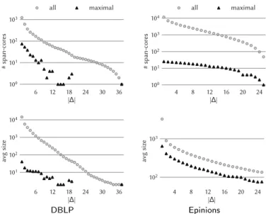
Hence, a span-core is recognized as maximal if it is not dominated by another span-core both on the order k and the span ∆. Differently from the innermost core (i.e., the core of the highest order) in the classic core decomposition, which is unique, in our temporal setting the number of maximal span-cores is O(|T |2), as, in the worst case, there may be one maximal span-core for every temporal interval. However, as observed in empirical temporal-network data, maximal span-cores are always much less than the overall span-cores: the difference is usually one order of magnitude or more. The second problem we tackle in this work is to compute the maximal span-cores of a temporal graph.
Problem 2 (Maximal Span-core Mining) Given a temporal graph G, find the set of all maximal (k, ∆)-cores of G.
Clearly, one could solve Problem 2 by solving Problem 1 and filtering out all the non-maximal span-cores. However, an interesting yet challenging question is whether one can exploit the maximality condition to develop faster algorithms that can directly extract the maximal ones, without computing all the span-cores. We provide a positive answer to this question in Section 5.
4
Algorithms: computing all span-cores
In this section we devise algorithms for computing a complete span-core decom-position of a temporal graph (Problem 1).
A na¨ıve approach. As stated in Observation 1, for a fixed temporal interval
∆ v T , mining all span-cores Ck,∆ is equivalent to computing the classic core
decomposition of the graph G∆ = (V, E∆). A na¨ıve strategy is thus to run a
core-decomposition subroutine [8] on graph G∆ for each temporal interval ∆ v
T . Such a method has time complexity O(P
∆vT(|∆| × |E|)), i.e., O(|T |
A more efficient algorithm. Looking at Figure 1 one can observe that the na¨ıve algorithm only exploits one dimension of the containment property: it starts from each point on the top level, i.e., from cores of order 1, and goes down vertically with the classic core decomposition. Based on Proposition 1, it is possible to design a more efficient algorithm that exploits also the “horizontal containment” relationships.
Example 1 Consider core C1,[0,2]in Figure 1: by Proposition 1 it holds that it is a subset of both C1,[0,1] and C1,[1,2]. Therefore, to compute C1,[0,2], instead of starting from the whole V , one can start from C1,[0,1]∩ C1,[1,2]. Starting from a much smaller set of vertices can provide a substantial speed-up to the whole computation.
This observation, although simple, produces a speed-up of orders of magni-tude as we will empirically show in Section 7. The next straightforward corollary of Proposition 1 states that, not only C1,[0,2]⊆ C1,[0,1]∩ C1,[1,2], but this is the best one can get, meaning that intersecting these two span-cores is equivalent to intersecting all span-cores structurally containing C1,[0,2].
Corollary 1 Given a temporal graph G = (V, T, τ ), and a temporal interval ∆ = [ts, te] v T , let ∆+ = [min{ts+ 1, te}, te] and ∆− = [ts, max{te− 1, ts}]. It holds that
C1,∆ ⊆ (C1,∆+∩ C1,∆−) =
\
∆0v∆ C1,∆0.
Example 2 Consider again C1,[0,2] in Figure 1: Proposition 1 states that it
is a subset of C1,[0,0], C1,[0,1], C1,[1,1], C1,[1,2], C1,[2,2]. Corollary 1 suggests that there is no need to intersect them all, but only C1,[0,1] and C1,[1,2]: in fact, C1,[0,1]⊆ C1,[0,0]∩ C1,[1,1] and C1,[1,2]⊆ C1,[1,1]∩ C1,[2,2].
The main idea behind our efficient Span-cores algorithm (whose pseudocode is given as Algorithm 1) is to generate temporal intervals of increasing size (starting from size one) and, for each ∆ of width larger than one, to initiate the core decomposition from (C1,∆+∩ C1,∆−), i.e., the smallest intersection of cores containing C1,∆(Corollary 1). The intervals to be processed are added to queue Q, which is initialized with the intervals of size one (Lines 2–3): these are the only intervals for which no other interval can be used to reduce the set of vertices from which the core decomposition is started, thus they have to be initialized with the whole vertex set V . The algorithm utilizes a map A that, given an interval ∆, returns the set of vertices to be used as a starting set of the core decomposition on ∆. The algorithm processes all intervals stored in Q, until Q has become empty (Lines 4–16). For every temporal interval ∆ extracted from Q, the starting set of vertices is retrieved from A[∆] and the corresponding set of edges is identified (Line 6). Unless this is empty, the classic core-decomposition algorithm [8] is invoked over (A[∆], E∆[A[∆]]) (Line 8) and its output (a set of span-cores of span ∆) is added to the ultimate output set C (Line 9).
Algorithm 1: Span-cores
Input: A temporal graph G = (V, T, τ ). Output: The set C of all span-cores of G.
1 C ← ∅; Q ← ∅; A ← ∅
2 forall t ∈ T do
3 enqueue [t, t] to Q; A[t, t] ← V
4 while Q 6= ∅ do
5 dequeue ∆ = [ts, te] from Q
6 E∆[A[∆]] ← {(u, v) ∈ E∆| u ∈ A[∆], v ∈ A[∆]}
7 if |E∆[A[∆]]| > 0 then
8 C∆← core-decomposition(A[∆], E∆[A[∆]])
9 C ← C ∪ C∆
10 ∆1= [max{ts− 1, 0}, te]; ∆2= [ts, min{te+ 1, tmax}]
11 forall ∆0 ∈ {∆1, ∆2} | ∆06= ∆ do
12 if A[∆0] 6= null then
13 A[∆0] ← A[∆0] ∩ C1,∆
14 enqueue ∆0 to Q
15 else
16 A[∆0] ← C1,∆
Afterwards, the two intervals, denoted ∆1 and ∆2, for which C1,∆ can be
used to obtain the smallest intersections of cores containing them (Corollary 1) are computed at Line 10. For ∆1(and analogously ∆2), we check whether A[∆1] has already been initialized (Line 12): this would mean that previously the other “father” (i.e., smallest containing core) of C1,∆1 has been computed, thus we can intersect C1,∆ with A[∆1] and enqueue ∆1 to be processed (Lines 13–14). Instead, if A[∆1] was not yet initialized, we initialize it with C1,∆(Line 16): in this case ∆1 is not enqueued because it still lacks one father to be intersected before being ready for core decomposition. This procedural update of Q ensures that both fathers of every interval in Q exist and have been previously computed, thus no a-posteriori verification is needed.
Example 3 Consider again the search space in Figure 1. Algorithm 1 first processes the intervals [0, 0], [1, 1], [2, 2], and [3, 3]. Then, it intersects C1,[0,0] and C1,[1,1]to initialize C1,[0,1], intersects C1,[1,1]and C1,[2,2]to initialize C1,[1,2], and intersects C1,[2,2] and C1,[3,3] to initialize C1,[2,3]. Then, it continues with the intervals of size 3: it intersects C1,[0,1] and C1,[1,2] to initialize C1,[0,2] and so on.
The next theorem formally shows soundness and completeness of our Span-cores algorithm.
The algorithm generates and processes a subset of temporal intervals X ⊆
{∆ | ∆ v T }. For every interval ∆ ⊆ X , it computes all span-cores C∆ =
{C1,∆, C2,∆, . . . , Ck∆,∆} defined on ∆ by means of the core-decomposition sub-routine on the graph (A[∆], E∆[A[∆]]). The set of vertices A[∆] is equivalent to (C1,∆+∩C1,∆−) because of Line 13 (Corollary 1) and the fact that ∆ is enqueued (Line 14) only when both fathers have been processed and the intersection done. The correctness of doing the classic core decomposition is guaranteed by Obser-vation 1.
As for completeness, it suffices to show that the intervals ∆ /∈ X that have not been processed by the algorithm do not yield any span-core. The algorithm generates all temporal intervals size by size, starting from those of size one and then going to larger sizes. This is done by maintaining the queue Q. As said
above, an interval ∆ is enqueued as soon as both C1,∆+ and C1,∆− have been
processed. Thus, an interval ∆ is not in X only if either C1,∆+ or C1,∆− does not exist. In this case C1,∆ and all other Ck,∆ do not exist as well.
Discussion. Algorithm 1 exploits the “horizontal containment” relationships only at the first level of the search space. For a given ∆, once the restricted starting set of vertices has been defined for k = 1, the traditional core decom-position is started to produce all the span-cores of span ∆. In other words, for k > 1 only the “vertical containment” is exploited. Consider the span-core
C3,[1,2] in Figure 1: we know that it is a subset of C2,[1,2] (“vertical” ) and of
C3,[1,1] and C3,[2,2] (“horizontal” ). One could consider intersecting all these
three span-cores before computing C3,[1,2]. We tested this alternative approach, but concluded that the overhead of computing intersections and data-structure maintenance was outweighing the benefit of starting from a smaller vertex set. The worst-case time complexity of Algorithm 1 is equal to the na¨ıve ap-proach, however, in practice, it is orders of magnitude faster, as shown in Sec-tion 7.
5
Algorithms: computing maximal span-cores
In this section we focus on Problem 2: computing the maximal span-cores of a temporal graph.
A filtering approach. As anticipated above, a straightforward way of solving this problem consists in filtering the span-cores computed during the execution of Algorithm 1, so as to ultimately output only the maximal ones. This can easily be accomplished by equipping Algorithm 1 with a data structure M that stores the span-core of the highest order for every temporal interval ∆ v T that has been processed by the algorithm. Moreover, at the storage of a
span-core Ck,∆ in M, the span-cores previously stored in M for subintervals of the
temporal interval ∆ and with the same order k are removed from M. This removal operation, together with the order in which span-cores are processed, ensures that M eventually contains only the maximal span-cores.
ef-ficient algorithm that extracts maximal span-cores directly, without computing complete core decompositions, passing over more peripheral ones, and without generating all temporal cores. This is a quite challenging design principle, as it contrasts the intrinsic structural properties of core decomposition, based on which a core of order k is usually computed from the core of order k −1, thus making the computation of the core of the highest order as hard as computing the overall decomposition. Nevertheless, thanks to theoretical properties that relate the maximal span-cores to each other, in the temporal context such a challenge can be achieved. In the following we discuss such properties in de-tail, by starting from a result that has already been discussed above, but only informally.
Consider the classic core decomposition in a standard (non-temporal) graph G (Definition 1) and let Ck∗[G] denote the innermost core of G, i.e., the non-empty k-core of G with the largest k.
Lemma 1 Given a temporal graph G = (V, T, τ ), let CM be the set of all
maximal span-cores of G, and Cinner = {Ck∗[G∆] | ∆ v T } be the set of
innermost cores of all graphs G∆. It holds that CM ⊆ Cinner.
Every Ck,∆ ∈ CM is the innermost core of the non-temporal graph G∆: else,
there would exist another core Ck0,∆ 6= ∅ with k0 > k, implying that Ck,∆ ∈/ CM.
Lemma 1 states that each maximal span-core is an innermost core of a G∆,
for some temporal interval ∆ v T . Hence, there can exist at most one maximal span-core for every ∆ v T (while an interval ∆ may not yield any maximal span-core). The key question to design an efficient maximal-span-core-mining
algorithm thus becomes how to extract innermost cores of the graphs G∆more
efficiently than by computing the full core decompositions of all G∆. The answer to this question comes from the result stated in the next two lemmas (with Lemma 2 being auxiliary to Lemma 3).
Lemma 2 Given a temporal graph G = (V, T, τ ), and three temporal intervals ∆ = [ts, te] v T , ∆0= [ts−1, te] v T , and ∆00= [ts, te+1] v T . The innermost core Ck∗[G∆] is a maximal span-core of G if and only if k∗> max{k0, k00} where k0 and k00 are the orders of the innermost cores of G∆0 and G∆00, respectively. The “⇒” part comes directly from the definition of maximal span-core (Def-inition 3): if k∗ were not larger than max{k0, k00}, then Ck∗[G∆] would be dominated by another span-core both on the order and on the span (as both
∆0 and ∆00 are superintervals of ∆). For the “⇐” part, from Lemma 1 and
Proposition 1 it follows that max{k0, k00} is an upper bound on the maximum order of a span-core of a superinterval of ∆. Therefore, k∗ > max{k0, k00} im-plies that there cannot exist any other span-core that dominates Ck∗[G∆] both on the order and on the span.
Lemma 3 Given G, ∆, ∆0, ∆00, k0, and k00 defined as in Lemma 2, let eV = {u ∈ V | d∆(V, u) > max{k0, k00}}, and let Ck∗[G∆[ eV ]] be the innermost core of
Algorithm 2: Maximal-span-cores
Input: A temporal graph G = (V, T, τ ).
Output: The set CM of all maximal span-cores of G.
1 CM ← ∅
2 K0[t] ← 0, ∀t ∈ T
3 forall ts∈ [0, 1, . . . , tmax] do
4 t∗ ← max{te∈ [ts, tmax] | E[ts,te] 6= ∅}
5 k00← 0 6 forall te∈ [t∗, t∗−1, . . . , ts] do 7 ∆ ← [ts, te] 8 lb ← max{K0[te], k00} 9 Vlb← {u ∈ V | d∆(V, u) > lb} 10 E∆[Vlb] ← {(u, v) ∈ E∆| u ∈ Vlb, v ∈ Vlb} 11 C ← innermost-core(Vlb, E∆[Vlb]) 12 k∗← order of C 13 if k∗> lb then 14 CM ← CM ∪ {C} 15 k00← max{k00, k∗}; K0[te] ← max{K0[te], k00}
G∆[ eV ]. If k∗ > max{k0, k00}, then Ck∗[G∆[ eV ]] is a maximal span-core; other-wise, no maximal span-core exists for ∆.
Lemma 2 states that, to be recognized as a maximal span-core, the innermost core of G∆ should have order larger than max{k0, k00}. This means that, if the innermost core of G∆is a maximal span-core, all vertices u /∈ eV cannot be part
of it. Therefore, G∆ yields a maximal span-core only if the innermost core of
subgraph G∆[ eV ] has order k∗ > max{k0, k00}. Lemma 3 provides the basis of our efficient method for extracting maximal span-cores. Basically, it states that, to verify whether a certain temporal interval ∆ = [ts, te] yields a maximal span-core (and, if so, compute it), there is no need to consider the whole graph G∆, rather it suffices to start from a smaller subgraph, which is given by all vertices whose temporal degree is larger than the maximum between the orders of the innermost cores of intervals ∆0 = [t
s− 1, te] and ∆00 = [ts, te+ 1]. This finding suggests a strategy that is opposite to the one used for computing the overall span-core decomposition: a top-down strategy that processes temporal intervals starting from the larger ones. Indeed, in addition to exploiting the result in Lemma 3, this way of exploring the temporal-interval space allows us to skip the computation of complete core decompositions of the whole “singleton-interval” graphs {G[t,t]}t∈T, which may easily become a critical bottleneck, as they are the largest ones among the graphs induced by temporal intervals. The Maximal-span-cores algorithm. Algorithm 2 iterates over all timestamps ts∈ T in increasing order (Line 3), and for each tsit first finds all the maximal span-cores that have span starting in ts. This way of proceeding ensures that a
span-core that is recognized as maximal will not be later dominated by another span-core. Indeed, an interval [ts, te] can never be contained in another interval [t0s, t0e] with ts < t0s. For a given ts, all maximal span-cores are computed
as follows. First, the maximum timestamp ≥ ts such that the corresponding
edge set E[ts,te] is not empty is identified as t∗ (Line 4). Then, all intervals ∆ = [ts, te] are considered one by one in decreasing order of te(Lines 6–7): this again guarantees that a span-core that is recognized as maximal will not be later dominated by another span-core, as the intervals are processed from the largest to the smallest. At each iteration of the internal cycle, the algorithm resorts to Lemma 3 and computes the lower bound lb on the order of the innermost core of G∆to be recognized as maximal, by taking the maximum between K0[te] and k00 (Line 8). K0 is a map that maintains, for every timestamp t ∈ [ts, t∗], the order of the innermost core of graph G∆0, where ∆0 = [ts−1, t] (i.e., K0[t] stores what in Lemmas 2–3 is denoted as k0). Whereas k00 stores the order of the innermost core of G∆00, where ∆00 = [ts, te+ 1]. Afterwards, the sets of vertices Vlband of edges E∆[Vlb] that comply with this lower-bound constraint are built (Lines 9–10), and the innermost core of the subgraph (Vlb, E∆[Vlb]) is extracted (Lines 11–12). Ultimately, based again on Lemma 3, such a core is added to the output set of maximal span-cores only if its order is actually larger than lb (Lines 13–14), and the values of k00 and K0[t
e] are updated (Line 15). Specifically, note that the order k∗ of core C may in principle be less than k00,
as C is extracted from a subgraph of G∆. If this happens, it means that the
actual order of the innermost core of G∆ is equal to k00. This motivates the update rules (and their order) reported in Line 15.
Theorem 2 Algorithm 2 is sound and complete for Problem 2.
The algorithm processes all temporal intervals ∆ v T yielding a non-empty edge set E∆, in an order such that no interval is processed before one of its superintervals: this guarantees that a span-core recognized as maximal will not be dominated by another span-core found later on. For every ∆ it extracts
a core C that is used as a proxy of the innermost core of graph G∆. C is
added to the output set CM only if Lemma 3 recognizes it as a maximal
span-core, otherwise it is discarded. This proves the soundness of the algorithm. Completeness follows from Lemma 1, which states that to extract all maximal span-cores it suffices to focus on the innermost cores of graphs {G∆| ∆ v T }, and Lemma 3 again, which states the condition for a proxy core C to be safely discarded because it is a non-maximal span-core.
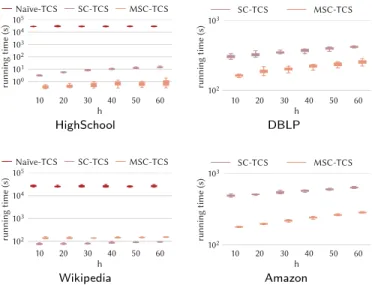
Discussion. The worst-case time complexity of Algorithm 2 is the same as the algorithm for computing the overall span-core decomposition, i.e., O(|T |2×|E|). It is worth mentioning that it is not possible to do better than this, as the output itself is potentially quadratic in |T |. However, as we will show in Section 7, the proposed algorithm is in practice much more efficient than computing the overall span-core decomposition and filtering out the non-maximal span-cores as, in this case, we avoid the visit of portions of the span-core search space and the computations are run over subgraphs of reduced dimensions.
To conclude, we discuss how the crucial operation of building the subgraph (Vlb, E∆[Vlb]) may be carried out efficiently in terms of both time and space. Consider a fixed timestamp ts∈ [0, . . . , tmax]. The following reasoning holds for every ts. Let E−(te) = E[ts,te]\ E[ts,te+1] be the set of edges that are in E[ts,te] but not in E[ts,te+1], for te∈ [ts, . . . , t∗−1]. As a first general step, for each ts, we compute and store all edge sets {E−(te)}te∈[ts,t∗−1]. These operations can be accomplished in O(|T |×|E|) overall time, because every E−(te) can be computed incrementally from E[ts,te] as E−(te) = {(u, v) ∈ E[ts,te] | τ (u, v, te+ 1) = 0}. Moreover, for any timestamp te, we keep a map D storing all vertices of G[ts,te] organized by degree. Specifically, the set D[k] contains all vertices having degree > k in G[ts,te]. Every vertex in D is thus replicated a number of times equal to its degree. This way, the overall space taken by D is O(|E|), i.e., as much space as G. D is initialized as empty (when te= t∗) and repeatedly augmented as te decreases, by a linear scan of the various E−(t
e). The overall filling of D (for all te) therefore takes O(|T | × |E|) time. Then, the desired Vlbcan be computed in constant time simply as Vlb= D[lb].
As for E∆[Vlb], for any te, we first reconstruct E[ts,te] as E[ts,te+1]∪ E−(te), having previously computed E[ts,te+1]. Note that storing all E−(te) takes O(|E|) space. That is why we store all E−(te) and reconstruct E[ts,te] afterward (in-stead of storing the latter, which would take O(|T | × |E|) space). E∆[Vlb] is ultimately derived by a linear scan of E
[ts,te], taking all edges in E[ts,te] having
both endpoints in Vlb. This way, the step of building E∆[Vlb] for all te takes again O(|T | × |E|) overall time.
6
Temporal community search
Community search in static graphs aims at finding a dense subgraph (commu-nity) containing a set of input query vertices [32, 46]. In the temporal setting it is very likely that the communities spanning the query vertices change over time. To be more precise, it may happen that a certain subgraph S is a well-representative community for the given query vertices Q, but only for a certain time interval ∆. Instead, for another time interval ∆0, a relevant community for Q might correspond to a completely different subgraph S0. For this reason, we formulate community search on temporal networks as the problem of finding h subgraphs (with h > 0 being an input parameter) containing the query vertices, together with their temporal span, such that the sum of the density of those sub-graphs is maximized and the union of their temporal spans corresponds to the whole input temporal domain. Among the many densities proposed in the liter-ature, here we follow the seminal work by Sozio and Gionis [74] on community search and adopt the minimum degree. Formally:
Problem 3 (Temporal Community Search) Given a temporal graph G = (V, T, τ ), a set Q ⊆ V of query vertices, and a positive integer h ∈ N+, find a set {hSi, ∆ii}hi=1 of h pairs such that (i) ∀1 ≤ i ≤ h : Q ⊆ Si ⊆ V , (ii)
S
1≤i≤h∆i= T , and (iii) the following is maximized:
h X
i=1 min
u∈Sid∆i(Si, u). (1)
The input integer h is a user-defined parameter that gives the analyst the flexibility of requiring a specific number of output temporal communities, which might vary from application to application.
6.1
Connection with Sequence Segmentation
Here we provide some theoretical insights into the Temporal Community Search problem. The main result we provide at the end of this subsection is an interesting connection with the well-established Sequence Segmentation problem [10]. As shown in the next subsections, such a result forms the basis for algorithmic design.
Let us first consider a single-interval variant of Problem 3: for a fixed tem-poral interval ∆, find a subgraph containing the input set Q of query vertices that maximizes the minimum temporal degree within ∆. Formally:
Problem 4 (Single Temporal Community Search) Given a temporal graph G = (V, T, τ ), a set Q ⊆ V of query vertices, and an interval ∆ v T , find
S∗= argmaxQ⊆S⊆V min
u∈Sd∆(S, u).
It is easy to see that solving Problem 4 corresponds to solving
minimum-degree-based community search on graph G∆. Therefore, a solution to
Prob-lem 4 can straightforwardly be computed by applying a standard result on minimum-degree-based community search, which states that the highest-order core containing all query vertices is a solution to that problem [7]. This finding is formalized next.
Definition 4 ((Q, ∆)-highest-order-span-core) Given a temporal graph G = (V, T, τ ), a set Q ⊆ V of query vertices, and an interval ∆ v T , the (Q, ∆)-highest-order-span-core of G, denoted CQ,∆∗ , is defined as the highest-order span-core among all span-span-cores of G with temporal span ∆ and containing all query vertices in Q. Let also v∗Q,∆ denote the order of CQ,∆∗ .
Fact 1 Given a temporal graph G = (V, T, τ ), a set Q ⊆ V of query vertices, and an interval ∆ v T , the (Q, ∆)-highest-order-span-core of G is a solution to Problem 4 on input hG, Q, ∆i.
Note that Problem 4 may have multiple solutions: CQ,∆∗ is only one of those
possibly many ones. CQ,∆∗ can be computed by running a core decomposition on
(static) graph G∆, and stopping it when the first core that does not contain all query vertices in Q has been encountered. Therefore, Problem 4 can be solved in O(|∆| × |E|) time.
In light of the above findings, an alternative yet equivalent way of formulating our Temporal Community Search problem is to ask for a segmentation (i.e., a partition) of the time domain T into a set {∆i}hi=1 of h intervals so as to
maximize the sum Ph
i=1vQ,∆∗ i of the orders of the (Q, ∆)-highest-order-span-cores of those identified intervals. Once such an optimal segmentation of T has been computed, the ultimate {hSi, ∆ii}hi=1 pairs are derived by simply setting Si= CQ,∆i∗ , ∀1 ≤ i ≤ h. Formally:
Problem 5 (Alternative formulation of Problem 3) Given a temporal graph G = (V, T, τ ), a set Q ⊆ V of query vertices, and a positive integer h ∈ N+, find a set {hSi, ∆ii}hi=1 of h pairs such that (i) ∀1 ≤ i ≤ h : Si = CQ,∆i∗ , (ii) {∆i}hi=1 is a partition of T , and (iii) the following is maximized:
h X
i=1 vQ,∆∗
i. (2)
Correspondence between Problem 3 and Problem 5 easily follows from Fact 1 and from the observation that for any feasible solution {hSi, ∆ii}hi=1 to Prob-lem 3 with overlapping intervals, there exists an overlapping-interval-free feasible solution with not smaller objective-function value. To see the latter, for any two overlapping intervals ∆iand ∆j, simply replace one of the two intervals, say ∆i, with ∆0i = ∆i\ (∆i∩ ∆j). As ∆0iv ∆i, it holds that vQ,∆∗ 0
i ≥ v
∗
Q,∆i, therefore the resulting overlapping-interval-free solution will have objective-function value greater than or equal to the objective-function value of the starting solution with overlapping intervals.
Thanks to the reformulation in Problem 5, it is immediate to observe that our Temporal Community Search problem is an instance of the well-established Sequence Segmentation problem, which asks for partitioning a sequence of numerical values into b segments so as to minimize the sum of the penalties (according to some penalty function) on each identified segment [10]:
Problem 6 (Sequence Segmentation [10]) Given a sequence X = (x0, x1, . . . , xmax) of numerical values, and a function p : {Y }Y vX→ R that assigns a penalty score
to every subsequence Y of X, partition X into a set {Xi}bi=1 of b subsequences such thatPb
i=1p(Xi) is minimized.
Fact 2 Temporal Community Search (Problem 3) on input hG = (V, T, τ ), Q, hi is an instance of Sequence Segmentation (Problem 6) with X = T , b = h, and ∀∆ v T : p(∆) = −vQ,∆∗ .
In the following two subsections we show how to exploit the result in Fact 2 (and a further important finding about maximal span-cores) to design efficient algorithms for our Temporal Community Search problem.
Algorithm 3: Temporal-community-search
Input: A temporal graph G = (V, E, T ), a set Q ⊆ V of query vertices, an integer h ∈ N+.
Output: A set {hSi, ∆ii}hi=1, where Q ⊆ Si⊆ V , ∀1 ≤ i ≤ h, and {∆i}hi=1 is a partition of T .
/* Initialization */
1 Compute vQ,∆∗ and CQ,∆∗ , ∀∆ v T , via Q-constrained span-core decomposition
2 P ← an empty (|T | × h)-dimensional matrix // Penalty matrix
3 R ← an empty (|T | × h)-dimensional matrix // Reconstruction matrix
4 forall t ∈ T do 5 P[t, 0] ← −v∗Q,[0,t] 6 R[t, 0] ← 0 /* Dynamic-programming step */ 7 forall t ∈ T do 8 forall i ∈ [1, h) do 9 P[t, i] ← min`∈[0,t]P[`, i − 1] − v∗Q,[`+1,t] 10 R[t, i] ← argmin`∈[0,t]P[`, i − 1] − v∗Q,[`+1,t]
/* Reconstruction of the solution */
11 ub ← tmax 12 forall i ∈ (h, 0] do 13 lb ← R[ub, i] 14 ∆i← [lb, ub] 15 ub ← lb − 1 16 forall i ∈ (h, 0] do 17 Si← CQ,∆∗ i
6.2
A basic algorithm (based on all span-cores)
Sequence Segmentation can be solved in O(|X|2× h + τp) time via
dy-namic programming [10], where τp is the overall time spent for computing the
penalty score of all subsequences of the input sequence X (according to the given penalty function p). Thanks to the connection shown in Fact 2, the dynamic-programming algorithm for Sequence Segmentation can be easily adapted to solve Temporal Community Search as well. The pseudocode of this al-gorithm – termed Temporal-community-search – is reported as Alal-gorithm 3, and described next.
The Temporal-community-search algorithm makes use of two (|T |×h)-dimensional matrices, i.e., P and R. Matrix P represents the penalty matrix. It contains, ∀t ∈ T , ∀i ∈ [0, h), the minimum cost of segmenting the sequence corresponding to the first t timestamps of T into i + 1 segments. As a result, P[tmax, h − 1] contains the objective-function value of the ultimate optimal solution to
Prob-lem 5. Matrix R is the reconstruction matrix. It provides information about the optimal segmentation, and is used at the end of the algorithm to reconstruct the output {∆i}hi=1. Note that the algorithm does not explicitly compute the Si subgraphs corresponding to the optimal ∆iintervals. In fact, as discussed above, each Si can be easily retrieved at the end of the algorithm, by simply setting it equal to the corresponding (Q, ∆i)-highest-order-span-core CQ,∆i∗ . According to Fact 2, the penalty score of an interval ∆ v T corresponds to −v∗Q,∆, i.e., the negative of the order of the (Q, ∆)-highest-order-span-core CQ,∆∗ . All individual v∗Q,∆values, for all ∆ v T , are efficiently computed altogether, at the beginning of the algorithm, via a “Q-constrained” variant of span-core decomposition (an alternative, but much less efficient strategy consists in computing every single v∗Q,∆from scratch, on the fly). Specifically, a simple (yet more efficient) variant of the span-core decomposition algorithm (Algorithm 1) is employed for this purpose, which outputs only those span-cores containing all the vertices in Q. This is easily achievable by stopping the core-decomposition subroutine, for ev-ery interval ∆ v T , as soon as a core not containing all quev-ery vertices in Q has been encountered.
The time complexity of Algorithm 3 is O(|T |2× h + τsc), where τsc is the time spent for computing the Q-constrained span-core decomposition of the input graph G.
6.3
A more efficient algorithm (based on maximal
span-cores)
A more efficient algorithm can be designed by noticing that, actually, one does not need to consider all timestamps in T in the dynamic-programming step.
Rather, focusing on a subset T∗ ⊆ T – which is properly defined based on
the maximal span-cores of the input graph, see next – allows for significantly reducing the dimensionality of the penalty matrix P and the reconstruction matrix R, hence the overall time complexity of the algorithm, without affecting optimality of the output solution. The following fact provides the theoretical basis for defining such a reduced temporal domain T∗.
Fact 3 Given a temporal graph G = (V, T, τ ) and a set Q ⊆ V of query vertices, let CM(Q) be the set of all Q-constrained maximal span-cores of G. For a tem-poral interval ∆ v T , it holds that v∗Q,∆= max{0, max{k | Ck,∆0 ∈ CM(Q), ∆ v ∆0}}.
Fact 3 states that the penalty score v∗Q,∆of an interval ∆ corresponds to the maximum among the orders of the Q-constrained maximal span-cores whose span includes ∆, if some exist. If an interval ∆ is not a subset of any span
of a Q-constrained maximal span-core, then vQ,∆∗ = 0. In that case,
there-fore, ∆ can be safely discarded, as it cannot be part of the optimal solution of the given Temporal Community Search problem instance (unless it is needed to fill possible “holes”, see below). The ultimate consequence of this finding is that the aforementioned reduced temporal domain T∗ is identified by
the timestamps covered by the spans of the maximal span-cores, along with auxiliary timestamps, which are needed to ensure a smooth execution of the dynamic-programming step, as well as a correct handling of some extreme cases.
Specifically, let D = {∆ v T | Ck,∆ ∈ CM(Q)} be the set of the spans of
the Q-constrained maximal span-cores of the input graph, and TD =S∆∈D∆
be the set of timestamps that are part of a span of a Q-constrained maximal span-core. The first two sets of auxiliary timestamps correspond to the times-tamps that immediately precede and succeed the intervals in D, i.e., the sets TD+ = {min{te+ 1, tmax} | [ts, te] ∈ D} and TD−= {max{ts− 1, 0} | [ts, te] ∈ D}, respectively. The timestamps in TD+and TD−(along with the last timestamp tmax of the input temporal domain T ) are needed to allow the dynamic-programming step to identify a solution that actually covers the whole temporal domain T (as per Condition (ii) of Problem 3). In particular, such timestamps may be interpreted as a trick to give the dynamic-programming step the flexibility to select “holes” (i.e., time intervals in-between two consecutive but not
neces-sarily contiguous timestamps in TD). Moreover, we define Tsup as the set of
the first h + 1 − |TD∪ TD− ∪ T +
D ∪ {tmax}| timestamps of T not contained in
TD∪ TD−∪ T +
D∪ {tmax}, i.e., Tsup= {ti ∈ T \ (TD∪ TD−∪ T +
D∪ {tmax}) | i ∈ [1, h + 1 − |TD ∪ TD− ∪ T
+
D ∪ {tmax}|]}. The timestamps in Tsup are further
auxiliary timestamps that are needed to return a correct h-sized solution when the timestamps in TD∪ TD−∪ T
+
D ∪ {tmax} are less than h + 1 (the minimum
number of timestamps required in T∗ to have a solution of size h). Note that
Tsup is nonempty only if |TD∪ TD−∪ T + D∪ {tmax}| < h + 1. Ultimately, T∗ is defined as T∗= TD ∪ TD+ ∪ T − D ∪ {tmax} ∪ Tsup.
The proposed more efficient method for Temporal Community Search, termed Efficient-temporal-community-search, is summarized in Algorithm 4 and described next. The first five lines of the algorithm are devoted to the
identifica-tion of T∗. As said above, matrices P and R have here reduced dimensionality
with respect to Algorithm 3: they are (|T∗| × h)-dimensional matrices, where
|T∗| ≤ |T |. A mapping function M is used to assign an index within [0, |T∗|)
to every timestamp in |T∗| (Line 6). Such a mapping is needed to have every
timestamp in |T∗| logically assigned to a row of matrices P and R. The rest of the algorithm resembles Algorithm 3, except for the fact that M is used every time that a row index has to be mapped to its corresponding timestamp (e.g., during the reconstruction of the solution).
An important point to clarify is that, during the execution of the
Efficient-temporal-community-search algorithm, we might need the penalty score v∗Q,∆
of intervals ∆ v T corresponding to non-maximal (Q-constrained) span-cores. Therefore, the algorithm needs the vQ,∆∗ score of all intervals ∆ v T . To com-pute these vQ,∆∗ scores (and, related to this, the set CM(Q) of Q-constrained maximal span-cores, at Line 1), there are two main options. The first one con-sists in computing the whole Q-constrained span-core decomposition (as done in Algorithm 3), keep the v∗Q,∆scores of all such cores, and eventually compute
corresponds instead to compute CM(Q) directly, without passing through the whole Q-constrained span-core decomposition. This may be carried out by run-ning a simple variant of the algorithm for computing maximal span-cores (Algo-rithm 2), where containment of query vertices is added as a further constraint. The computation of all the vQ,∆∗ scores comes for free during the execution of this algorithm for Q-constrained maximal span-cores: these scores can there-fore be retained by adding a few straightforward (constant-time) instructions to that algorithm. In our implementation we stick to the latter, as the Maximal-span-cores algorithm has been experimentally recognized as faster than the na¨ıve filtering approach in all tested datasets.
The time complexity of the proposed Efficient-temporcommunity-search al-gorithm is O(|T∗|2× h + τ
msc), with τmsc being the time spent in computing
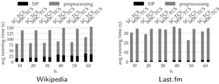
the Q-constrained maximal span-cores and the penalty scores v∗Q,∆. As in prac-tice (attested by our experiments) |T∗| |T |, the proposed Efficient-temporal-community-search algorithm is expected to be much more efficient than its na¨ıve counterpart, i.e., Algorithm 3.
6.4
Minimum community search
An instance of Temporal Community Search may admit several optimal solutions which might differ either in terms of output intervals {∆i}hi=1, or in terms of subgraphs assigned to the various identified intervals. More pre-cisely, the latter refers to the fact that two optimal solutions might find the same segmentation {∆i}hi=1 of the input temporal domain, but select different
subgraphs Si for any interval ∆i. Therefore, if the communities Si are not
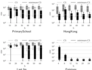
chosen carefully, they may result to be excessively large, not really cohesive, and containing redundant/outlying vertices. This is a well-recognized issue of minimum-degree-based community search [74]. At the same time, large com-munities might include more cohesive and denser subgraphs that still exhibit optimality. Motivated by this, in this subsection we devise a method to refine the communities originally found by our algorithms for Temporal Commu-nity Search, specifically attempting to minimize their size while preserving optimality. The main idea behind our refinement method is based on the fol-lowing result:
Proposition 2 (Community containment) Given a temporal graph G = (V, T, τ ), a set Q ⊆ V of query vertices, and a positive integer h ∈ N+, let {hSi, ∆ii}hi=1 be a solution to Problem 3 on input hG, Q, hi with Si correspond-ing to the (Q, ∆i)-highest-order-span-core of G, ∀i ∈ [1, h]. For every other solution {hSi0, ∆ii}hi=1 (referring to the same segmentation {∆i}hi=1) to Prob-lem 3 on input hG, Q, hi it holds that Si0 ⊆ Si, ∀i ∈ [1, h].
Let kibe the minimum degree of Si, i.e., ki= vQ,∆i∗ is the order of the (Q, ∆i )-highest-order-span-core. Assume that there exists a solution S0i to Problem 4 that is not contained in Si. This implies that (i) the minimum degree of a vertex of S0
as well. This violates the maximality condition of the definition of span-core, since, by hypothesis, Si corresponds to the (Q, ∆i)-highest-order-span-core of G.
The above proposition states that, given a solution {hSi, ∆ii}hi=1 to the
Temporal Community Search problem where every Si corresponds to the
(Q, ∆i)-highest-order-span-core of the input graph, one can focus on the various Sisolely to refine the output communities, as such Siare guaranteed to contain all optimal solutions of the underlying problem instance (while keeping the
segmentation {∆i}hi=1 fixed). Within this view, we formulate the following
optimization problem (which is a variant of Problem 4, with the additional constraint of requiring a smallest-sized solution):
Problem 7 Given a temporal graph G = (V, T, τ ), a set Q ⊆ V of query ver-tices, and an interval ∆ v T , let S∗ ⊆ V be the subset of vertices containing all the solutions to Problem 4 on input hG, Q, ∆i (according to what stated in Proposition 2). Find
Smin∗ = argmin{S|Q⊆S⊆S∗,minu∈Sd∆(S,u)≥min
u∈S∗d∆(S∗,u)}|S|.
Theorem 3 Problem 7 in NP-hard.
Consider (the optimization version of) the NP-hard mCST problem introduced by Cui et al. [21]: given a graph H = (VH, EH) and a query vertex q ∈ VH, find a minimum-sized subgraph that contains q, is connected, and maximizes the minimum degree. Given an instance hH, qi of the mCST problem, construct an instance hG, Q, ∆i of Problem 7 by defining G as composed by a single temporal snapshot corresponding to graph H, ∆ as a singleton interval composed of the single timestamp of G, and setting Q = {q}. It is straightforward to see that solving Problem 7 on input hG, Q, ∆i is equivalent to solving mCST on input hH, qi, as the constraint about connectedness is automatically satisfied in Problem 7 for the special case of a single query vertex.
As Problem 7 is NP-hard, we devise a heuristic that is inspired to the greedy one proposed for the Minimum Community Search problem in [7]. The proposed heuristic is outlined in Algorithm 5 and described next. In the pseudocode and in the following we denote as k∗and k∗minthe minimum degree of S∗ and Smin∗ , respectively, and as neigh∆(S, u) the neighbors of a vertex u ∈ V in the subgraph induced by S ⊆ V and ∆ v T . Algorithm 5 iteratively adds vertices to the solution Smin∗ according to a priority queue P . Priorities of vertices in P are defined based on a score that measures how promising a vertex
is for making the current solution Smin∗ reach the optimal minimum degree.
Specifically, the score of a vertex u ∈ S∗ is defined as: score(u) = score+(u) − score−(u), where
score+(u) = |{v ∈ neigh∆(Smin∗ , u) | d∆(Smin∗ , v) < k ∗}|; score−(u) = max{0, k∗− d∆(Smin∗ , u)}.
score+(u) is the gain effect of adding u to Smin∗ , while score−(u) is the penalty effect. In particular, score+(u) counts the number of neighbors of u in Smin∗ that would benefit from the inclusion of u to Smin∗ , i.e., that have degree less than k∗. On the other hand, score−(u) represents the number of neighbors of u still required in Smin∗ so that u has degree at least k∗. The algorithm starts by adding the query vertices to the queue P with priority +∞, in order to ensure that they will be selected at the very beginning. At each iteration of the main cycle of the algorithm (starting at Line 4), the vertex u exhibiting the highest priority is dequeued from P and is added to the solution Smin∗ . As a consequence, a couple of updates are performed. First, u’s neighbors not in the priority queue P are added to it (Lines 8-9). Note that this is the only step of the algorithm where the score of a vertex is computed from scratch and stored in A, a map that keeps the scores of all vertices in P up-to-date during the whole execution of the algorithm. The second update consists in recomputing the score of every v’s neighbor w in the queue, if a vertex v ∈ Smin∗ has reached the desired minimum degree k∗ after the addition of u.
7
Experiments
In this section we present an experimental evaluation to empirically assess the performance of all the proposed methods. Specifically, we focus on whole span-core decomposition (Section 7.1), maximal span-span-cores (Section 7.2), characteri-zation of the extracted span-cores (Section 7.3), and temporal community search (Section 7.4).
Datasets. We use eleven real-world datasets recording timestamped interac-tions between entities. For each dataset we select a window size to define a discrete time domain, composed of contiguous timestamps of the same dura-tion, and build the corresponding temporal graph. If multiple interactions oc-cur between two entities during the same discrete timestamp, they are counted as one. The characteristics of the resulting temporal graphs, along with the selected window sizes, are reported in Table 1.
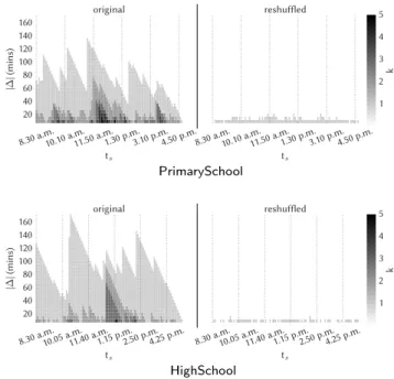
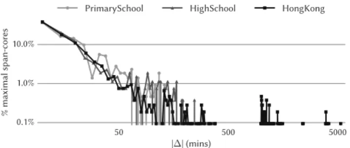
The three smallest datasets were gathered by using wearable proximity sen-sors in schools, with a temporal resolution of 20 seconds. PrimarySchool2 con-tains the contact events between 242 volunteers (232 children and 10 teachers) in a primary school in Lyon, France, during two days [76]. HighSchool2describes the close-range proximity interactions between students and teachers (327 indi-viduals overall) of nine classes during five days in a high school in Marseilles, France [61]. HongKong reports the same kind of interactions for a primary school in Hong Kong, whose population consists of 709 children and 65 teachers divided into thirty classes, for eleven consecutive days [71].
ProsperLoans3represents the network of loans between the users of Prosper, a marketplace of loans between privates. Last.fm3 records the co-listening ac-tivity of the Last.fm streaming platform: an edge exists between two users if
2sociopatterns.org 3konect.cc
![Figure 1: Search space: for a temporal span ∆ = [t s , t e ], the (k, ∆)-core is depicted as a node labeled “k, [t s , t e ]”](https://thumb-eu.123doks.com/thumbv2/123doknet/14620614.733701/10.918.276.637.183.466/figure-search-space-temporal-span-core-depicted-labeled.webp)