A Performance Study of various Brain Source Imaging Approaches

HAL Id: hal-00990273

https://hal.archives-ouvertes.fr/hal-00990273v2

Submitted on 9 Jul 2014

HAL is a multi-disciplinary open access

archive for the deposit and dissemination of

sci-entific research documents, whether they are

pub-lished or not. The documents may come from

teaching and research institutions in France or

abroad, or from public or private research centers.

L’archive ouverte pluridisciplinaire HAL, est

destinée au dépôt et à la diffusion de documents

scientifiques de niveau recherche, publiés ou non,

émanant des établissements d’enseignement et de

recherche français ou étrangers, des laboratoires

publics ou privés.

A Performance Study of various Brain Source Imaging

Approaches

Hanna Becker, Laurent Albera, Pierre Comon, Rémi Gribonval, Fabrice

Wendling, Isabelle Merlet

To cite this version:

Hanna Becker, Laurent Albera, Pierre Comon, Rémi Gribonval, Fabrice Wendling, et al.. A

Per-formance Study of various Brain Source Imaging Approaches. ICASSP 2014 - IEEE International

Conference on Acoustics, Speech and Signal Processing, May 2014, Florence, Italy. pp.5910-5914,

�10.1109/ICASSP.2014.6854729�. �hal-00990273v2�

A PERFORMANCE STUDY OF VARIOUS BRAIN SOURCE IMAGING APPROACHES

H. Becker

, L. Albera

, P. Comon

, R. Gribonval

, F. Wendling

, I. Merlet

(1) Univ. Nice Sophia Antipolis, CNRS, I3S, UMR 7271, F-06900 Sophia Antipolis, France

(2) GIPSA-Lab, CNRS UMR5216, Grenoble Campus, St Martin d’Heres, F-38402;

(3) INSERM, U1099, Rennes, F-35000, France;

(4) Universit´e de Rennes 1, LTSI, Rennes, F-35000, France;

(5) INRIA, Centre Inria Rennes - Bretagne Atlantique, France.

ABSTRACT

The objective of brain source imaging consists in reconstruct-ing the cerebral activity everywhere within the brain based on EEG or MEG measurements recorded on the scalp. This re-quires solving an ill-posed linear inverse problem. In order to restore identifiability, additional hypotheses need to be im-posed on the source distribution, giving rise to an impressive number of brain source imaging algorithms. However, a thor-ough comparison of different methodologies is still missing in the literature. In this paper, we provide an overview of priors that have been used for brain source imaging and conduct a comparative simulation study with seven representative algo-rithms corresponding to the classes of minimum norm, sparse, tensor-based, subspace-based, and Bayesian approaches. This permits us to identify new benchmark algorithms and promis-ing directions for future research.

Index Terms— EEG, MEG, inverse problem, source lo-calization, priors

1. INTRODUCTION

Electroencephalography (EEG) and magnetoencephalogra-phy (MEG) are two multi-sensor systems that are routinely used for the diagnosis and management of some diseases such as epilepsy or for the understanding of the brain functions in neuroscience research. The EEG/MEG measurements (X ∈ RN ×T), acquired with N sensors positioned on the scalp for T time samples, constitute a linear mixture of brain sources (S ∈ RD×T) in the presence of noise (N ∈ RN ×T):

X = GS + N. (1)

The mixture is characterized by the lead field matrix (G ∈ RN ×D), which can be computed given a model of the head

H. Becker was supported by Conseil R´egional PACA and by CNRS. The work of P. Comon was funded by the FP7 European Research Council Programme, DECODA project, under grant ERC-AdG-2013-320594. The work of R. Gribonval was funded by the FP7 European Research Council Programme, PLEASE project, under grant ERC-StG-2011-277906. We also acknowledge the support of Programme ANR 2010 BLAN 0309 01 (project MULTIMODEL).

and a predefined source space that is spanned by D dipoles with fixed positions inside the brain [1]. We assume in this paper that the source space consists of dipoles that are lo-cated on the cortical surface with orientations perpendicular to this surface [2]. The objective of brain source imaging con-sists in reconstructing the sources S based on the surface mea-surements X. However, as the number of dipoles (∼ 10000) generally exceeds the number of sensors (∼ 100), the source imaging problem is ill-posed. In order to restore identifiabil-ity, additional hypotheses about the sources have to be made. After several decades of research, giving rise to an im-pressive number of algorithms [3, 4, 5, 6], the source imaging problem is still one of the major challenges in biomedical en-gineering. Based on various priors, the proposed techniques pursue different methodological approaches, comprising min-imum norm, sparse, tensor-based, Bayesian, and subspace-based methods. However, a thorough comparison including algorithms of all these approaches is still missing. In this pa-per, we fill this gap by providing a classification of differ-ent algorithms based on the exploited priors and conducting a simulation study in which we compare seven representative algorithms of different classes: sLORETA [7], MCE [8], VB-SCCD [9], MxNE [10], STWV-DA [11], Champagne [12], and 4-ExSo-MUSIC [13]. This permits us to identify new benchmark algorithms and directions for further research.

2. HYPOTHESES

The hypotheses that are exploited to solve the brain source imaging problem can be distinguished into three categories: hypotheses that apply to the spatial, the temporal, and the spatio-temporal distribution of the sources. In the following, we provide an overview and a short description of the priors which have been used in brain source imaging.

2.1. Hypotheses on the spatial distribution

S1) Minimum energy The power of the sources is physio-logically limited. A popular approach thus consists in identi-fying the spatial distribution of minimum energy [14, 7].

S2) Minimum energy in a transform domain As the spa-tial distribution of the sources is unlikely to contain abrupt changes, it can be assumed to be smooth [15]. In practice, this is achieved by constraining the Laplacian of the source spatial distribution to be of minimum energy.

S3) Sparsity In practice, it is often reasonable to assume that only a small fraction of the source dipoles contributes to the measured signals of interest in a significant way. The signals of the other source dipoles are thus expected to be approxi-mately zero, leading to the concept of sparsity [8].

S4) Sparsity in a transformed domain If the number of ac-tive dipoles exceeds the number of sensors, the source distri-bution is not sufficiently sparse for standard methods based on sparsity to yield accurate results, leading to too focused source estimates. In this context, another idea consists in transforming the sources into a domain where their distribu-tion is sparser than in the original source space and imposing sparsity in the transformed domain [9].

S5) Separability in space and wavevector of the space-wavevector content For each superficial distributed source, one can assume that the space-wavevector matrix at each time point, which is obtained by computing a local spatial Fourier transform of the measurements, can be factorized into a func-tion that depends on the space variable only and a funcfunc-tion that depends on the wavevector variable only [16]. The space and wavevector variables are thus said to be separable, allow-ing for the use of tensor decomposition methods.

S6) Gaussian joint probability density function with pa-rameterized spatial covariance This prior assumes the source signals to be random variables that follow a Gaus-sian distribution with a spatial covariance matrix that can be described by a linear combination of a certain number of basis covariance functions [6, 12]. This combination is characterized by so-called hyperparameters, which have to be identified in the source imaging process.

2.2. Hypotheses on the temporal distribution

T1) Smoothness Since the autocorrelation function of the sources of interest usually has a full width at half maximum of several samples, the temporal distribution of the sources can be assumed to be smooth [10].

T2) Sparsity in a transformed domain This assumption im-plies that the source signals admit a sparse representation in a transformed domain, which can, for example, be achieved by a wavelet or Gabor transform applied to the temporal di-mension of the data [17]. The transformed signals can then be modeled using a small number of basis functions or atoms, which are determined by the source imaging algorithm. T3) Pseudo-periodicity with variations in amplitude If the recorded data comprises recurrent events like a repeated time pattern that can be associated to the sources of interest, such as interictal epileptic spikes, one can exploit the repetitions as

an additional diversity [18]. This permits us to employ tensor-based methods.

T4) Separability in time and frequency of the time-frequency content Under certain conditions such as os-cillatory signals, the time and frequency variables of data transformed into the time-frequency domain (for example, by applying a wavelet transform to the measurements) can be as-sumed to separate (cf. hypothesis S4)) [19]. This hypothesis gives rise to tensor-based approaches for source separation. T5) Non-zero higher-order marginal cumulants Regard-ing the measurements as realizations of a vector of random variables, this hypothesis is required when resorting to statis-tics of order higher than two, that offer a better performance and identifiability than approaches based on second order statistics [13]. It is generally verified in practice, as the sig-nals of interest usually do not follow a Gaussian distribution. 2.3. Hypotheses on the spatio-temporal distribution ST) Synchronous dipoles Contrary to point sources, which can be modeled by a single dipole, distributed sources are composed of a certain number of grid dipoles. These dipoles can be assumed to transmit synchronous signals [13].

3. ALGORITHMS

In this section, we classify seven representative algorithms based on the hypotheses that they exploit. Furthermore, we briefly describe the characteristics of each method.

sLORETA sLORETA [7] belongs to the class of minimum norm estimates (MNE) [14, 20], which exploit hypothesis S1) by minimizing the L2-norm regularized cost function:

L(s) = ||x − Gs||2₂+ λ||s||2₂ (2) where x and s correspond to columns of X and S, respec-tively. The first term on the right hand side of (2) is referred to as the data fit term, while the second term is called the reg-ularization term. The regreg-ularization parameter λ manages a balance between both terms. The particularity of sLORETA consists in providing a source estimate that is normalized with respect to the source covariance, leading to an unbiased solu-tion in the case of a single dipole source.

MCE The minimum current estimate (MCE) algorithm [8] has been developed to overcome the problem of blurred source reconstructions encountered with MNE and is based on hypothesis S3). In order to provide focused source es-timates, it replaces the regularization term in (2) by the sparsity-inducing L1-norm, ||s||1. This leads to a convex

optimization problem, for which identifiability conditions and efficient algorithms are available.

VB-SCCD The VB-SCCD algorithm [9] imposes sparsity on the variational map, which characterizes variations in am-plitude from one dipole source to adjacent dipole sources. This leads to a piecewise constant spatial distribution of the

sources. To apply hypothesis S4), a regularization term of the form ||Ts||1is used, where T is a transformation matrix

which implements the variation operator.

MxNE The mixed norm estimate (MxNE) [10] combines the hypotheses S3) and T1), leading to a spatially sparse, but tem-porally smooth source distribution. To achieve this, a mixed L1,2-norm regularization term is employed, leading to the

cost function:

L(S) = ||X − GS||2F+ λ||S||1,2. (3)

STWV-DA The space-time-wavevector based disk algo-rithm (STWV-DA) [11] belongs to the class of tensor-based approaches and proceeds in two steps: i) the separation of dif-ferent distributed sources using tensor decomposition based on hypotheses ST) and S5) (alternatively, one could exploit hypothesis T3) or T4)) and ii) the identification of grid dipoles characterizing each distributed source using hypothesis S4). To construct a third order tensor, a local spatial Fourier trans-form is applied to the measurements, leading to space-time-wavevector data. The tensor is then decomposed using the canonical polyadic decomposition [21], which permits to identify a vector of spatial characteristics for each distributed source. Subsequently, to identify the dipoles belonging to each distributed source, this vector is compared to the spatial characteristics of elementary (circular) distributed sources whose union should fit the expected distributed source. Champagne The Champagne algorithm [12] is an empirical Bayesian approach and assumes that the sources at each time point are described by a zero-mean Gaussian random vector of covariance Cscorresponding to hypothesis S6). The main

step of the algorithm consists in estimating the covariance Cs

from the data. This is achieved by an optimization process that requires an estimate of the noise covariance matrix. Once the matrix Csis known, it permits to directly derive an

esti-mate of the signals. In the absence of noise and for a source space with sufficiently high resolution, Champagne has been shown to provide a perfect source reconstruction.

4-ExSo-MUSIC The 4-ExSo-MUSIC algorithm [13] is a representative of the class of subspace-based methods and exploits the 4-th order cumulants of the measurements, thus relying on assumption T5). Exploiting the orthogonality be-tween the 4-th order signal and noise subspaces of the quadri-covariance matrix, 4-ExSo-MUSIC identifies the elements of a dictionary of potential distributed sources (assumption ST)) that best describe the measurements based on a metric. The dictionary is constructed in the same way as for STWV-DA, thus also using hypothesis S4). The estimated sources are ob-tained as a union of a certain number of dictionary elements, determined after thresholding the 4-ExSo-MUSIC metric.

4. SIMULATIONS

To compare the performances of the different source imag-ing algorithms, we apply them to realistic simulated data in

the context of epileptic EEG activity. We consider a realistic head model with three compartments representing the brain, the skull, and the scalp. The source space is composed of 19626 dipoles located on the cortical surface. The lead field matrix describing the propagation to 91 electrodes is com-puted numerically using a boundary element method. The epileptic source regions are modeled by patches which con-sist of adjacent grid dipoles. Highly correlated, physiolog-ically realistic epileptiform spike-like signals are generated for all dipoles belonging to a patch using a coupled neuronal population model [22]. To simulate epileptic activity spread-ing from one brain region to another, for scenarios with two patches, we use the same activities except for a time delay de-pending on the distance between the patches. All dipoles that do not belong to a patch are considered as generators of back-ground activity. The SNR of epileptic and backback-ground activ-ity is adjusted to realistic values. After spatially prewhiten-ing the data based on the noise covariance matrix, we apply the sLORETA, MCE, MxNE, VB-SCCD, STWV-DA, Cham-pagne, and 4-ExSo-MUSIC source imaging algorithms to the data of 10 epileptic spikes, which are concatenated for 4-ExSo-MUSIC and averaged for the other algorithms. To eval-uate the source localization results, we employ the distance of localization error (DLE) [23], which is defined as follows:

DLE = 1 2Q X k∈I min `∈ ˆI ||rk−r`||+ 1 2 ˆQ X `∈ ˆI min k∈I||rk−r`||. (4)

Here, I and ˆI denote the original and estimated sets of indices of all grid dipoles belonging to an active patch, Q and ˆQ are the numbers of original and estimated active grid dipoles, and rkdenotes the position of the k-th source dipole. The DLE is

averaged over 50 realizations, obtained with different spike-like signals and varying background activity.

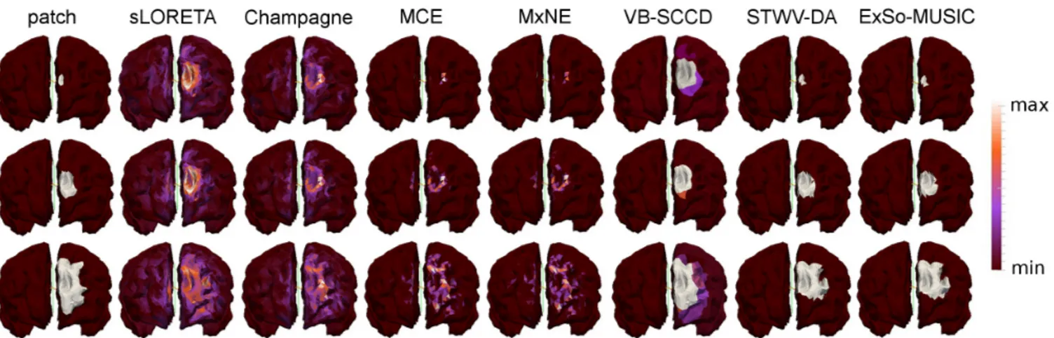
First, we study the influence of the patch size on the source localization results. To this end, we vary the size of a patch located in the superior frontal gyrus (SupFr), consider-ing 10, 100, and 400 grid dipoles, which corresponds to 0.5, 5, and 20 cm2of the cortical surface. Fig. 1 shows the origi-nal patches and a typical example of the reconstructed source configurations obtained by the different source imaging al-gorithms. sLORETA and Champagne yield similar results, which are blurred for the smallest patch and do not permit to accurately determine the spatial extent of the patches. MCE and MxNE provide very focal source estimates and are not suited to recover the size of the patch either. VB-SCCD over-estimates the size of the smallest patch, recovering a much larger source region. However, for medium to large patches, it provides good estimates of the patches. STWV-DA and 4-ExSo-MUSIC yield similar source reconstructions that are very close to the ground truth for the small and medium patch and slightly worse for the large patch. These results are also reflected by the DLE values shown in Table 1. Overall, the best performances are achieved for the patch of medium size. Second, we examine three scenarios with two patches,

Fig. 1. Original patch and source configurations estimated with different source imaging algorithms for the patch SupFr com-posed of 10, 100, and 400 dipoles.

Table 1. DLE (in cm) of source imaging algorithms for different scenarios

scenario sLORETA Champagne MCE MxNE VB-SCCD STWV-DA 4-ExSo-MUSIC

SupFr, small size 3.62 5.15 4.80 4.94 3.30 0.41 0.65

SupFr, medium size 1.97 2.51 2.95 3.03 0.53 0.43 0.44

SupFr, large size 5.45 3.38 4.02 4.78 0.89 1.14 1.15

InfFr+SupFr, small dist. 2.55 3.21 3.71 3.58 1.16 0.73 0.85

InfFr+InfPa, medium dist. 2.97 3.31 3.51 3.52 1.23 0.59 0.61

SupFr+SupOcc, large dist. 2.49 2.63 2.95 3.11 0.44 0.77 0.63

composed of 100 dipoles each and all located on the left hemi-sphere: patches InfFr and SupFr (inferior frontal and superior frontal gyri) with small distance, patches InfFr and InfPa (in-ferior frontal and in(in-ferior parietal gyri) with medium distance, and patches SupFr and SupOcc (superior frontal and superior occipital gyri) with large distance. Due to limited space, we only provide the results in terms of DLE, summarized in Table 1. While most methods show a tendency to yield somewhat improved source estimates for larger patch distance, the DLE does not decrease systematically with increasing distance for all algorithms and the source imaging performance seems to depend more on the patch position and form than the distance between two active patches. However, these results show that there is a gap between the performance of sLORETA, Cham-pagne, MCE, and MxNE, which achieve a DLE between 2.5 and 3.7 cm for the three scenarios, and the DLE of VB-SCCD, STWV-DA, and 4-ExSo-MUSIC, that is smaller than 1.3 cm. This is due to the fact that VB-SCCD, STWV-DA, and 4-ExSo-MUSIC permit to identify distributed sources, contrary to sLORETA, Champagne, MCE, and MxNE, as has also be-come apparent in the previous simulation.

5. CONCLUSIONS

In this paper, we have proposed a classification of differ-ent source imaging algorithms based on the hypotheses that

are imposed on the temporal and spatial distributions of the sources. To illustrate the use of various hypotheses, we have provided a short presentation of seven representative algorithms, whose performance has been compared in a sim-ulation study. This study has demonstrated the superior per-formance of VB-SCCD, STWV-DA, and 4-ExSo-MUSIC for the recovery of distributed sources as compared to sLORETA, Champagne, MCE, and MxNE. Among the latter four meth-ods, we have observed that sLORETA generally leads to the best performance. Moreover, we noticed that most algo-rithms (except for STWV-DA and 4-ExSo-MUSIC) require spatial prewhitening or an estimate of the noise covariance in order to yield accurate results. Therefore, the best overall performance, both in terms of robustness and accuracy, is achieved by STWV-DA. Further studies should be conducted to confirm these results.

To further enhance the performance, one could consider integrating the steps of two-step procedures such as STWV-DA into one single step in order to process all the available in-formation and constraints at the same time. Another promis-ing perspective for future research consists in explorpromis-ing dif-ferent combinations of a priori information, for example, by merging successful strategies of different recently established source imaging approaches, such as tensor-based, subspace-based, or Bayesian approaches and sparsity.

6. REFERENCES

[1] A. Gramfort, Mapping, timing and tracking cortical ac-tivations with MEG and EEG: Methods and application to human vision, Ph.D. thesis, Telecom ParisTech, 2009. [2] A. M. Dale and M. I. Sereno, “Improved localization of cortical activity by combining EEG and MEG with MRI cortical surface reconstruction: a linear approach,” Journal of Cognitive Neuroscience, vol. 5, no. 2, pp. 162–176, 1993.

[3] S. Baillet, J. C. Mosher, and R. M. Leahy, “Electromag-netic brain mapping,” IEEE Signal Processing Maga-zine, vol. 18, no. 6, pp. 14–30, Nov. 2001.

[4] C. M. Michel, M. M. Murray, G. Lantz, S. Gonzalez, L. Spinelli, and R. Grave De Peralta, “EEG source imag-ing,” Clinical Neurophysiology, vol. 115, no. 10, pp. 2195–2222, Oct. 2004.

[5] R. Grech, T. Cassar, J. Muscat, K. P. Camilleri, S. G. Fabri, M. Zervakis, P. Xanthopoulos, V. Sakkalis, and B. Vanrumste, “Review on solving the inverse problem in EEG source analysis,” Journal of NeuroEngineering and Rehabilitation, vol. 5, Nov. 2008.

[6] D. Wipf and S. Nagarajan, “A unified Bayesian frame-work for MEG/EEG source imaging,” NeuroImage, vol. 44, pp. 947 – 966, 2009.

[7] R. D. Pascual-Marqui, “Standardized low resolution brain electromagnetic tomography (sLORETA): techni-cal details,” Methods and Findings in Experimental and Clinical Pharmacology, 2002.

[8] K. Uutela, M. Hamalainen, and E. Somersalo, “Visu-alization of magnetoencephalographic data using mini-mum current estimates,” NeuroImage, vol. 10, pp. 173 – 180, 1999.

[9] L. Ding, “Reconstructing cortical current density by ex-ploring sparseness in the transform domain,” Physics in Medicine and Biology, vol. 54, pp. 2683 – 2697, 2009. [10] E. Ou, M. Hamalainen, and P. Golland, “A distributed

spatio-temporal EEG/MEG inverse solver,” NeuroIm-age, vol. 44, 2009.

[11] H. Becker, L. Albera, P. Comon, M. Haardt, G. Birot, F. Wendling, M. Gavaret, C. G. B´enar, and I. Merlet, “EEG extended source localization: tensor-based vs. conventional methods,” submitted to NeuroImage, 2013. [12] D. Wipf, J. Owen, H. Attias, K. Sekihara, and S. Na-garajan, “Robust Bayesian estimation of the location, orientation, and time course of multiple correlated neu-ral sources using MEG,” NeuroImage, vol. 49, pp. 641 – 655, 2010.

[13] G. Birot, L. Albera, F. Wendling, and I. Merlet, “Local-isation of extended brain sources from EEG/MEG: the ExSo-MUSIC approach,” NeuroImage, vol. 56, pp. 102 – 113, 2011.

[14] M. S. H¨am¨al¨ainen and R. J. Ilmoniemi, “Interpreting magnetic fields of the brain: Estimates of current distri-butions,” Technical Report TKK-F-A559, Helsinki Uni-versity of Technology, Finland, 1984.

[15] R. D. Pascual-Marqui, C. M. Michel, and D. Lehmann, “Low resolution electromagnetic tomograph: A new method for localizing elecrical activity in the brain,” Int. Journal of Psychophysiology, vol. 18, pp. 49 – 65, 1994. [16] H. Becker, P. Comon, L. Albera, M. Haardt, and I. Mer-let, “Multi-way space-time-wave-vector analysis for EEG source separation,” Signal Processing, vol. 92, pp. 1021–1031, 2012.

[17] A. Gramfort, D. Strohmeier, J. Haueisen, M. Hamalainen, and M. Kowalski, “Time-frequency mixed-norm estimates: Sparse M/EEG imaging with non-stationary source activations,” NeuroImage, vol. 70, pp. 410 – 422, 2013.

[18] J. M¨ocks, “Decomposing event-related potentials: a new topographic components model,” Biological Psy-chology, vol. 26, pp. 199–215, 1988.

[19] F. Miwakeichi, E. Martinez-Montes, P. A. Valdes-Sosa, N. Nishiyama, H. Mizuhara, and Y. Yamaguchi, “De-composing eeg data into space-time-frequency compo-nents using parallel factor analysis,” NeuroImage, vol. 22, pp. 1035–1045, 2004.

[20] R. D. Pascual-Marqui, “Review of methods for solv-ing the EEG inverse problem,” International Journal of Bioelectromagnetism, vol. 1, no. 1, pp. 75 – 86, 1999. [21] P. Comon, L. Luciani, and A. L. F. De Almeida,

“Ten-sor decompositions, alternating least squares and other tales,” Journal of Chemometrics, vol. 23, pp. 393–405, 2009.

[22] D. Cosandier-Rim´el´e, J.-M. Badier, P. Chauvel, and F. Wendling, “A physiologically plausible spatio-temporal model for EEG signals recorded with intrac-erebral electrodes in human partial epilepsy,” IEEE Transactions on Biomedical Engineering, vol. 54, no. 3, pp. 380–388, Mar. 2007.

[23] J.-H. Cho, S. B. Hong, Y.-J. Jung, H.-C. Kang, H. D. Kim, M. Suh, K.-Y. Jung, and C.-H. Im, “Evaluation of algorithms for intracranial EEG (iEEG) source imaging of extended sources: feasibility of using (iEEG) source imaging for localizing epileptogenic zones in secondary generalized epilepsy,” Brain Topography, , no. 24, pp. 91–104, 2011.