HAL Id: hal-00800656
https://hal.archives-ouvertes.fr/hal-00800656
Submitted on 14 Mar 2013
HAL is a multi-disciplinary open access
archive for the deposit and dissemination of sci-entific research documents, whether they are pub-lished or not. The documents may come from teaching and research institutions in France or abroad, or from public or private research centers.
L’archive ouverte pluridisciplinaire HAL, est destinée au dépôt et à la diffusion de documents scientifiques de niveau recherche, publiés ou non, émanant des établissements d’enseignement et de recherche français ou étrangers, des laboratoires publics ou privés.
Climate and Electoral Turnout in France
Christian Ben Lakhdar, Eric Dubois
To cite this version:
Christian Ben Lakhdar, Eric Dubois. Climate and Electoral Turnout in France. French Politics, Palgrave Macmillan, 2006, 4 (2), pp.137. �hal-00800656�
C
LIMATE AND ELECTORAL TURNOUT INF
RANCEChristian Ben Lakhdar
and Eric Dubois
Forthcoming in French Politics, volume 4, number 2 (August, 2006)
Abstract: It is commonly stated that the climate has an impact on electoral turnout. This
article aims to test this proposition that has not been scientifically proved in the French case yet. Using the last five parliamentary elections turnout data and the corresponding climatic data on the voting day, our study shows that rain has a depressing effect on turnout, whereas sunshine and high temperatures incite people to vote.
Keywords: climate; weather; vote; parliamentary election; turnout; France
ESSEC Doctoral program, 1, Avenue Bernard Hirsch, BP 105, 95021 Cergy-Pontoise cedex, France and MATISSE, University of Paris 1 Panthéon-Sorbonne, Maison des Sciences Economiques, 106-112, Boulevard de l‟Hôpital, 75647 Paris cedex 13, France. Tel.: +33.1.44.07.81.01 ; fax.: +33.1.44.07.81.09. Email: Christian.Benlakhdar@malix.univ-paris1.fr
LAEP, University of Paris 1 Panthéon-Sorbonne, Maison des Sciences Economiques, 106-112, Boulevard de l‟Hôpital, 75647 Paris cedex 13, France. Tel.: +33.1.44.07.81.01 ; fax.: +33.1.44.07.81.09. Email: Eric.Dubois@univ-paris1.fr
According to the U.S. Census Bureau, 0.6 % of the registered non voters in the U.S. elections of November 2000 stated that they didn‟t vote because of the “bad weather”1
. As in 2000, the number of the registered non voters was 18.7 millions2, that means that, if the survey is unbiased, 112.200 persons didn‟t vote because of the climatic conditions. Due to the close results of this election, no need to say that each vote was crucial. In the same fashion, after the record of abstention of the French presidential election of 2002, one could read in the newspaper Le Figaro: "the weather was fine in the whole of France that may have distracted voters of their electoral duty"3. This kind of arguments, extensively widespread in the media, suffers, at least in France, of a lack of strong scientifical foundations. Paradoxically, it seems that no study exists on the link between political life and climate whereas France is often pioneer in political science as well as in science of Earth. The English literature is more fertile4.
A first axis of research intends to study the impact of climatic conditions on the course of particular political events. Some studies show how climatic conditions can disrupt, or even differ, a transfer of power ceremony or an Inauguration Day5. It is not insignificant, especially if one considers that the cancellation of an investiture ceremony can for example delay the implementation of the newly elected President's policy. Thus, every presidential election year,
Weatherwise magazine publishes an article whose object is to describe the weather on
Inauguration Day (see Ludlum 1984 and Hughes 1988, 1996). March 4th, the traditional date of the ceremony, was frequently the theatre of terrific climatic conditions. Thus, half of the investiture ceremonies between 1789 and 1933 took place under a bad weather (snow, rain and chill). Roosevelt inaugurated in 1937 a new date of investiture fixed by the Constitution 20th amendment to January 20th of the year following the election. Alas for him, this ceremony was the rainiest of the whole history! The change of date hasn't therefore been sufficient to break this surprising correlation, the icy temperature of January 20th, 1985 even forcing Ronald Reagan to take oath sheltered from the Capitol‟s dome6
.
The second axis of research on the interactions between climate and politics7 tries to verify the existence of an impact of the climate on electoral results. The latters can be the score achieved by political parties or the rate of turnout. It is interesting to note that the first study aiming to explain the vote ever published takes into account the impact of climatic conditions (Barnhart, 1925). The author shows that bad climatic conditions (drought, rain…) reveal deficiencies in infrastructures (transportation, equipment…), deficiencies of which political leaders are held responsible for. The contestation can go up to the creation of
suppose that climatic conditions affect economic conditions through an increase of certain prices such as prices of agricultural products. This inflation, seen negatively, would decrease the vote in favor of the incumbent (Pearson and Myers, 1948)8.
Relative to the turnout issue, climatic conditions can offset the decision of some voters to vote or not. For example, a rainy weather will simply discourage some voters and divert them from their electoral duty. It has been studied notably by Ludlum (1984), Merrifield (1993) and Knack (1994). Merrifield (1993) shows that rain, defined as the total of precipitations fallen in the biggest city of every state the Election Day, played a significantly negative role on the turnout of American voters for the 1982 congressional elections9. The gap between the temperature on the election day and the “normal” temperature is also significantly negatively related to the turnout. Therefore, to summarize, the more it rains, the less people vote and the more the temperature departs of the normal, the less people vote.
Studies of Ludlum (1984) and Knack (1994) go further in claiming that climatic conditions influence the scores obtained by political parties. Thus, a fact of the American political folklore is that rain favors Republicans. The relationship would be the following: rain has a depressing effect on the turnout and the abstention helps Republicans since Democrats abstain more frequently. Steve Knack tests this proposition by confronting polls achieved in 1984, 1986 and 1988 among electors and abstentionists to the climatic conditions that prevailed on the voting day. His findings are the following ones: bad climatic conditions discourage effectively some voters but this kind of abstention, and even the abstention in general, doesn't favor Republicans. Ludlum (1984), using historical examples, shows that climatic conditions in populated states as California or Florida can affect the American presidential election‟s national result by influencing the abstention in these states. Thus, in 1960, J.F. Kennedy won some states as Illinois or Missouri by a narrow margin, eventhough these states were more prone to vote for the Republican candidate R. Nixon. In those two states, one noted that climatic conditions were especially bad on the voting day. Republican voters, residing mainly in farming counties, sulked polls but not Democrat voters which lived mostly in the big cities of those states.
Another category of studies aims at examining the impact of climatic conditions on the result of incumbent parties. At the beginning of the XXth century, Marshall (1927)10 had studied the correlation between precipitations fallen during the four years preceding the Presidential election and the incumbent party electoral results. This paper is outstanding because its author proposes a theoretical foundation. According to him, in the agricultural-based states, climatic conditions determine the quality of the harvests that determines the
voters‟ level of satisfaction: "Scant rainfall means poor crops, poor crops mean hard times, and hard times mean discontent" (Marshall, 1988: 265). The electoral mechanism is like a punition/reward system: voters reward the incumbent party for good harvests and punish it otherwise11. R. Marshall, after having studied the 25 American presidential elections between 1825 and 1924, finds that for the 12 elections having lead to a change of party in power, 11 elections took place in years of weak precipitations. On the 13 elections won by the incumbent, 11 elections took place in years of abundant rains. In other words, the total of precipitations fallen during the four years of the presidential term allowed to forecast the future President in a correct way in near of 90% of the elections between 1825 and 1924.
Let's note that other articles show a surprising correlation without obvious theoretical foundations. Thus, one learns that in Boston, for the last forty years, it snowed two times more when the President was Democrat than when the President was Republican (D‟Aleo, 1998)!
As we can see through this short survey of the literature, the French case has not been tackled yet, even briefly. Our study aims to fill this gap. Firstly, we present the theoretical foundations of the abstention. After having described the variables, the data and the methodology, we then show the estimations and the results of our study. Some extensions are explored before closing by some conclusive remarks.
Theoretical Foundations of Turnout
Why do people vote and why they don‟t? The turnout or the abstention to vote can be identified as a rational choice problem. To make this choice, voters do a cost / benefit analysis of the act of voting that can be described by the following relation12:
R = B.p + D-C
where R denotes their expected utility. B is the gain derived from the political program and p the probability that an individual's vote is decisive by permitting to change the result of the election. D represents non contingent gains of turnout as the respect of a certain ethics or the affirmation of the political system efficiency (Riker and Ordeshook, 1968). C represents the costs of voting. These are essentially opportunity costs as the collect of information on
political programs or the fact to go to the polls13. The voter decides to vote if the gains are greater than the costs and abstains otherwise14.
As in Merrifield (1993) and Knack (1994), the hypothesis advanced in our study is that climatic variables, while modifying the costs, influence the voter's decision to vote or not. However, these studies remain mute on the shapes that such a modification can take. In order to be more precise, we decompose the costs as follow:
j i C
C
C
where Ci represents the opportunity costs before the Electoral Day as, for example, the follow-up of the campaign or the study of programs and Cj represents the opportunity costs
on the electoral day as the displacement to the polls. The climate is not a cost in itself (i.e. it doesn't belong to Ci nor toCj) but modify the perception ofCj15. For instance, two persons
having the same Cj and facing the same climatic conditions on the voting day could adopt a
different attitude facing to the voting act.
The empirical study may allow us to verify that the climate, while modifying the perception of some costs related to the vote, influences the decision to vote and then has an impact on the electoral turnout. The following development specifies the variables, the data and the methodology used.
The Empirical Model
The dependent variable, notedTURN i,t, is the turnout in the French departments for the first round of the five parliamentary elections since 198616. We have then four choices to justify: the electoral unit, the relevant round, the level of elections and the studied period.
France is subdivided in “regions”, each of them, subdivided in several “departments”. Each department is composed by several electoral districts. There are in metropolitan France 22 regions, 96 departments, and 555 electoral districts. The district level has been moved apart because too few data were available to define our independent variables17. We have chosen department because it is a more homogeneous electoral territory than the region. Indeed, most of regions show important disparities. For example, in the region "Aquitaine" that traditionnally votes for the Left, the department "Pyrénées-Atlantiques" votes always for
the Right. In the same way, the department "Côtes-d'Armor" votes for the Left but the region which it belongs to, the region "Bretagne", votes for the Right. These disparities are by large softened inside a department even if one can observe some exceptions as the department "Lozère" where northern voters support the Right and southern ones the Left. By estimating the same model (same dependent variable, same explanatory variables, same period) at different levels of data (national, regional, departmental), Dubois and Fauvelle-Aymar [2004] shown a clear superiority of the departmental model at least in terms of vote forecasting.
Furthermore, our study only concerns the first ballot. First, this choice permits to avoid the occurrence of particular cases that entails a more complicated modeling as triangular contests (left/right/extreme-right), fratricidal duels (left/left or right/right), single candidate at the second round or even absence of second round. Second, at the first round, the electoral supply (i.e. the number of candidates) is larger and then the turnout is less constrained.
We have chosen parliamentary elections because these elections are, with the presidential ones, the more important in the French citizens‟ eyes. We have not aggregated these two types of elections because, according to us, this aggregation rests on the too strong hypothesis that determinants of turnout at the parliamentary and at the presidential elections are the same.
We started our study in 1986 to insure of constituencies homogeneity. Since that year, the number of electoral district is remained unchanged18.
We retained six explanatory variables. The first one is a trend variable that captures the political weariness that characterizes the French voter since near twenty-five years as shown on the figure 1.
[ FIGURE 1 ABOUT HERE ]
This weariness finds its origins mainly in the multiplication of scandals involving politicians, in a possible lack of representativeness and in the repetition of electoral ballots (28 in 10 years for all types of elections!). The expected sign of the coefficient of this variable, noted TREND, will be therefore negative.
The second variable is a dummy variable that takes into account the special features of the 1986 ballot. For this election, there was a single round what probably leads to a higher turnout. Furthermore the fact that regional elections were organized the same day constituted another incentive to go to polls. The variable will be noted DUM1986 and will take 1 in 1986 and 0 otherwise. We expect a positive sign for the coefficient of this variable. At first glance, the
The following explicative variable is a variable that catches the economic situation. For example, when macroeconomic performances are poor, two arguments can be advanced. According to the first one, turnout is higher because some voters that usually abstain go to polls to sanction the ruling majority. The second argument, opposed to the first, is that voters who support the incumbent prefer to abstain rather to vote against her. We have retained the unemployment rate to account for the economic situation. More precisely, UNEM1 is the difference in the unemployment rate between the quarter of the election and the quarter before, UNEM2 is the difference in the unemployment rate between the quarter of the election and four quarters before (that is on one year), and UNEM3 is the difference in the unemployment rate between the quarter of the election and eight quarters before (that is on two years). We define three variables to allow a more or less high degree of memory to the French voter. The expected sign is undetermined according to the aforementioned arguments. The variable could then have a positive sign (as in Merrifield, 1993) or a negative sign (as in Fauvelle-Aymar et
al., 2000). In the case where the two effects opposed, the variable should be non significant.
The three other independent variables are the climatic variables on the Electoral day: temperature, precipitations and sunshine.
The first problem to deal with these variables is the geographical heterogeneity. For example, 20 degrees are not experienced in the same way in a northern department than in a southern department. In order to erase these disparities and therefore to capture the exceptional character of some precipitations, temperatures or sunshine, we chose to withdraw the long term trend of our climatic data. For this, we withdrew the “climatic standard” that is the monthly average on the period 1951-1980.
We then use the following variables:
t i
PRE , : height in millimeters of the precipitations fallen between 6 a.m. and 6 p.m. on the voting day minus the long term tendency observed on the period 1961-199019.
t i
TEMP , : arithmetic mean of the temperature in Celsius degrees measured at 6 a.m. and the temperature in Celsius degrees measured at 6 p.m. on the voting day minus the long term tendency observed on the period 1961-1990.
t i
SUN , : “sunshine ratio” defined as “length of sunshine / length of the astronomical day x 100” on the voting day minus the long term tendency observed on the period 1951-1980.
If intuitively, the climatic variable that influences the turnout the most should be precipitations, there is here a problem linked to their frequency since a drizzle falling continuously will discourage voters more presumably than a big temporary shower20.
The sunshine ratio is a good indicator because, by its construction, it permits to account for what we call a “good weather” or a “bad weather”. Indeed, for example, a sunshine ratio of 90 % for a city means that it was shiny 90 % of the day and not that there was a strong sunshine during a small part of the day.
Numerous other variables explaining the turnout exist (see, among others, Blais and Dobrzynska (1998) and the articles quoted above). These variables are essentially socio-demographical factors that affect turnout in the long run: age, level of education, religion, etc21. They explain why a department systematically has a higher turnout rate than another. To capture these spatial disparities, we estimate a fixed-effects model22. In this kind of models, the intercept term varies from a department from another. This allows us to take into account the long run specificities of each department (see Dubois and Fauvelle-Aymar, 2004).
The model to estimate will be:
t , i t , i 6 t , i 5 t , i 4 t , i 3 i 2 t 1 i t ,
i c TREND DUM1986 UNEMj TEMP PRE SUN
TURN
where j = 1, 2, 3, for UNEM according to the definition retained. Let‟s turn to the description of the sample and to the presentation of the estimation results now.
Sample and Estimation Results
There are 96 departments in France but our sample is reduced since only 90 of them have a “reference meteorological station”23
. The second filter is the availability of the climatic standard: only 43 departments simultaneously offer the three climatic standards24. Our final sample then includes these 43 departments on 5 elections, that is a total of 215 observations25.
The table 1 shows some descriptive statistics26.
[ TABLE 1 ABOUT HERE ]
The figures below plot the turnout against our three climatic variables27.
[ FIGURE 2 ABOUT HERE ]
[ FIGURE 4 ABOUT HERE ]
These figures conceal precious information on the expected sign of the climatic variable resumed in table 2.
[ TABLE 2 ABOUT HERE ]
The estimation leads to28:
[ TABLE 3 ABOUT HERE ]
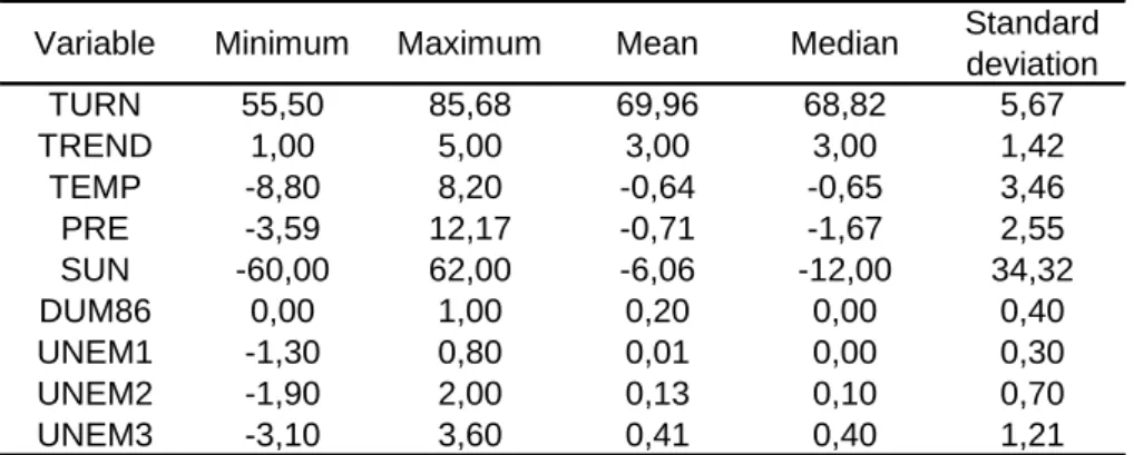
Immediately we see in columns 1 and 2 that the unemployment variable is not statistically significant at a 10 % level29. We have then removed this variable (column 4). But in column 1 to 4, all the climatic variables are simutaneously included and that can lead to a multicolinearity problem. Intuitively, we can think for example that higher the sunshine ratio is, higher the temperature is or higher the sunshine ratio is, lower precipitations are. To tackle this problem, we have run three regressions with a single climatic variable (columns 5, 6, 7). As we can see, all the climatic variables are significant at a 1 % level, their coefficients are broardly the same than in column 4 and they keep the same sign. All of this indicate that the multicolinearity, if it exists, is not a very important issue. Moreover, simple correlations between turnout and weather variables are rather weak: 0.39 for temperatures, 0.15 for precipitations, and 0.13 for the sunshine ratio. To clear this point, we have estimated auxiliary regressions as suggested by Gujarati (2003). Results are shown in table 4.
[ TABLE 4 ABOUT HERE ]
Partial correlations are all significant but not very high. The rule is that if no R² obtained from auxiliary regressions is higher than the overall R² (table 3, column 4), multicolinearity is not a troublesome problem (Gujarati, 2003, 361). This is the case here. We remark in table 4 that the three highest R² are the ones associated to the UNEMs variables. This can explain the non significativity of UNEM1 and UNEM2 and the fact that TREND is no longer significant when included with UNEM3 (that is significant at a 1 % level).
We turn to the interpretation of the results. According to the discussion above, we focus on equation 4. All the variables have the expected sign and are significant at a 1 % level
except the trend variable that is significant at a 5 % level. For this late variable, the coefficient indicates that the turnout decreases of 0.25 point from one election to another. For example, this negative trend costs 2.5 points in 2002 (since the value of the trend in 2002 is 5). The fact that there was a single round for the legislative election and two ballots the same day in 1986 has increased the turnout of about 10 points for this election. Then, it seems that the climate has an important impact on the turnout at French parliamentary elections. TEMP i,t and
t , i
SUN have a positive impact on the turnout: a hot and/or a sunny day enhance people to vote. More precisely, if we compare to a normal day (in a climatic sense), 3 degrees more increase the turnout of about one point and 4 hours of sun more30 increase the turnout of a quarter point. The variable PRE i,t has the expected negative sign: the more it rains, the less people vote. 6 millimeters of precipitations more lead to a decrease of the turnout of about 1 point (compared to a normal day, once again).
Further results
The first point we want to mention in this section concerns a possible threshold effect for our climatic variables. If on the graphs above, we have detected a linear relation between each climatic variable and the turnout, one can think that the relation can be nonlinear. What we have shown is that when the climate is bad, people stay at home and abstain and when the weather is fine, they go to polls. But what happen when climatic conditions are exceptionally good? One can think that they prefer to go to the beach instead of to spend their time to vote. Thus, in the newspaper Corse Matin on the 03/13/1989, one could read: "One can say that flooded by a more-than-vernal sun, voters had amply sulked the polls". Statistically speaking, the relation between turnout and climate wouldn't be a strait line but a U-shaped curve. To investigate this possibility, we have estimated a nonlinear functional form for each of our climatic variable. We have considered a degree up to two in order to avoid difficulties in the interpretation31: 2 x x y
where y is the turnout and x a climatic variable. To test if this nonlinear form is better than the linear one, we have performed a F-test (Greene, 1997, 343-344). This test is adequate because in each case, linear or nonlinear, the model can be estimated by OLS. If it is obvious in the linear case, few words have to be said on the nonlinear one. The model above can be written:
x z y
where observations for z are the squares of the observations of x. As Kennedy (1992, 94) pointed out, the equation is nonlinear in variables but linear in parameters. In this case, it can be estimated by OLS.
The table 5 gives the R² for each estimated functional form and the Fisher statistics.
[ TABLE 5 ABOUT HERE ]
Then we accept a nonlinear form for temperatures only. Here is the graph with the curve:
[ FIGURE 5 ABOUT HERE ]
As expected, we have an inversed-U-shaped curve: low temperatures as high temperatures have a depressing effect on turnout. Why is it specific to this variable? For precipitations, according to the linear relation, the more it rains, the less people vote. There is no place here for a U-shaped curve: it doesn't make sense to state that a strong rain enhances people to go to polls. For the sunshine, it's trickier. In particular, how to explain that temperatures and sunshine are disconnected? In fact, it's quite straightforward: we can have both a cold and sunny weather or both a warm and cloudy weather. Then sunshine is not a necessary and sufficient condition to go to the beach or to the park; temperature has to be high as well.
The final step with this nonlinear modelling is to estimate the complete model. Column 8 table 3 gives the results.
All the results above are related to estimations on departmental data. We have justified this choice previously by the lack of economic variables at a finer level. Since we removed these variables for multicolinearity problems, we now can estimate our model with district data.
We have identified electoral districts where departmental meteorological stations are located and we have saved the turnout in these electoral districts. In the special case where the departmental meteorological station was in a city composed by several districts, we have summed registered voters on one side and effective voters on an another side to obtain a global turnout rate32. To finish with the description of the dependent variable, just note that the correlation between the turnout at the departmental level and the turnout at the district level is 88 %33. This high but not perfect correlation can indicate a possible loss of
information when we explain the turnout at the departmental level only. It also means that we can expect different results.
Let‟s turn to the explicative variables now. We keep all our preceding variables except DUM1986 that accounts for specificities of the 1986 ballot. We have already seen two features of this election that may influence the turnout: a single round and two elections on the same day. But this election also gave rise to others institutional changes. First, it was the first time of the fifth Republic that a legislative election occurred at the proportional rule and not at the majority one. Secondly, and more important for our purpose, voters didn‟t elect one deputy in each district but voted for a departmental list (one list by party). The rank of the lists in each department allocated a certain number of seats to the National Assembly. One can consider that for this election, the district was the department as the whole. This last feature lead us to remove DUM1986 since this variable has sense at the departmental level only34.
The results of the district estimation are shown in table 3, column 9. At the first glance, one can see that the coefficients‟ size is comparable to the ones obtain column 4, except for the trend variable for which the coefficient is much larger in the district estimation than in the department estimation. One can explain this difference by arguing that districts in our sample are mainly localized in big cities (since the meteorological station is the departmental station of reference) and that the negative trend is most dominant in big cities since in rural areas turnout is sticky because of the “social control”35.
All climatic variables are correct-signed and significant at a level of 10 % or more. The size of coefficients indicates that the impact of climatic variable is globally stronger than in the department regression (i.e. coefficients are higher in absolute value for two variables from three). It does not mean that the voting behaviour has changed with the level of data but simply that the focus on a smaller territory unit gives more precise information. It is not surprising since the climate measured in the departmental meteorological station of reference is not necessary the climate in the rest of the department.
The coefficient interpretation is close to what have been done above. Comparatively to a normal day, 5 degrees more increase the turnout of about two points, 4 hours of sun more36 increase the turnout of one point, and 7 millimeters of precipitations more leads to a decrease of the turnout of about 1 point.
the rain helps Republicans in the U.S.? This supposes two relations: a relation between climate and turnout that we have now demonstrated and a relation between turnout and vote.
According to Fauvelle-Aymar et al. (2000), in France, abstention penalizes left-wing parties37. The explanation may reside in the likeness of abstainers and left-wing voters. Indeed, these two groups present several common features: rather young, rather weak attachment to the Catholic religion, rather low study level… (see Mossuz-Lavau, 1997). If this link is correct, while having a depressive effect on the abstention, good weather would favour the Left. Dubois (2005) tells another story. His data give no support for a link between turnout and Left vote but acknowledge a positive relation between turnout and incumbent vote38. The theoretical arguments have been presented earlier in this paper. Basically, vote is higher in the case of good macroeconomic performances because some voters that usually abstain go to polls to reward the ruling majority and vote is lower in the case of poor macroeconomic performances because some voters that usually support the incumbent prefer to abstain instead of voting against her.
The table 6 gives the correlations between the turnout and different measures of the vote in our sample39.
[ TABLE 6 ABOUT HERE ]
Turnout seems to help both the Left and the ruling majority (when moderate right are incumbent) but, as the column 3 reveals, the correlation between the turnout and the ruling majority vote is spurious. Most of this correlation is due to the correlation between the turnout and the left vote. It is also noteworthy to precise that in our sample the Left is the incumbent in 3 elections from 5 (1986, 1993, and 2002).
As good meteorological conditions enhance turnout and as turnout and left vote are positively correlated, then one can say that a nice climate helps the Left40.
Conclusion
In the media, it is commonly stated that the climate influences the electoral turnout. In this paper, this proposition has been tested for the last five French parliamentary elections. Data give a strong support to the impact of climatic conditions on turnout. Indisputably, the rain has a depressive effect on turnout whereas sunshine and high temperatures encourage it.
As peripheral results, we bring to light some specificities of the 1986 ballot and the trend in turnout is well caught.
The main econometric issues have been tackled as heteroskedasticity or multicolinearity what gives reliability to the model and trust in its results.
Moreover, these results seem robust since they hold whatever the level of data, department or district. A threshold effect has been found in temperatures: low temperatures as high temperatures enhance abstention. A hot day doesn‟t warrant a polls rush.
We hit here an agenda-setting problem: what is the optimal election date to maximize the turnout? The immediate answer would be on a nice day but it would be a wrong one. Indeed, our climatic variables are defined in difference with the standard normal. In other words, no matter it‟s -2° if the standard normal is -5°. The day has to be a nicer-than-usual day. It is then impossible to set an electoral calendar unless to be able to forecast the climate several months in advance.
We have also shown that there exists a positive link between turnout and Left vote. The main implication is that a fine weather favours left-wing parties. Then the Right (Left), when incumbent, would have to choose the election date so that it falls a bad (good) day. However we face here the same agenda-setting problem mentioned above: the day has to be a worse-than-usual (better-worse-than-usual) one.
Then, there is a positive evidence of a link between climate and turnout but no normative prescription. To have such recommendations, a control over climatic conditions is necessary. However, if Nature influences politics, politics does not influence Nature yet.
Acknowledgements
We thank Christine Fauvelle-Aymar, Abel François, and Pierre Martin for data provision and Mike Lewis-Beck for his trust in this paper. We are also grateful to an anonymous referee for having suggested valuable improvements to its first version.
Notes
1
Report on Voting and Registration in the Election of November 2000, page 10 (source:
3
Le Figaro, 06/17/2002, page 2.
4
It is hardly surprising with personages as Benjamin Franklin, inventor of the lightning conductor and writer of the American Declaration of Independence.
5
The Inauguration Day is the day of the President of the United States' investiture.
6
Senator Howard Baker even proposed to organize the next investiture ceremonies on Independence Day (July 4).
7
We do not deal with the case where extreme climatic conditions lead to the cancellation of the ballot as it was the case for example in Madagascar for the 1991 general elections.
8
In the light of this relation, it is therefore possible to find a causal foundation to the correlation between precipitations and inflation that Hendry (1980) judges spurious. In this famous paper, the author takes these two variables in example to show that correlation is not causality.
9
The aim of Merrifield (1993) is not to put in evidence the sole impact of the climate but to explain in details the turnout. In order to do so, he uses seventeen other explanatory variables including institutional variables, socio-demographic variables, etc.
10
This article, originally published in 1927 in Weatherwise, is reprinted in the same review in 1988.
11
This has been theorized by Key (1966).
12
Borrowed from Struthers and Young (1989).
13
For a more detailed survey on costs and gains to vote, see Aldrich (1993), and more specifically on the cost to go to polls, see Gimpel and Schuknecht (2003).
14
Some authors advanced the idea that the costs are always superior to the gains, mainly because of the weakness of p (Tullock, 1968). Since, in spite of that, people go effectively to the polls, there is a paradox known as "paradox of voting".
15
According to Rallings et al. (2003), the perception of the cost of voting can be modified by natural factors as the length of the day. In particular, going to the polls at dusk would have a supplementary psychological cost linked to the fear of the crime. The authors show then that abstention is larger in Winter than in Summer since the night falls earlier.
16
March 16, 1986, June 5, 1988, March 21, 1993, May 25, 1997, and June 9, 2002.
17
This problem of data availability explains why a pooled-data model by district hasn't existed in the French case yet (for the vote as for the turnout).
18
19
Since the climatic standard for precipitations is the total of precipitations fallen during the month, we have divided this total by the number of days in the month (31 if the elections hold in March, etc).
20
This problem can be solved in studying the intraday data and not daily data. But, if such data maybe exist for the climate, they are not available for the turnout.
21
For an econometric study that assesses the impact of these variables on turnout in the French case, see Fauvelle-Aymar and François (2005). Unfortunately, socio-demographic variables are not yearly available. Since data exist only for census years (that is, in our sample, 1990 and 1999), we have not taken these variables into account. One can also think to other short-term variables as holidays for example. When the ballot takes place during holidays, the turnout can be weaker since a lot of voters are not at home. We can't test this proposition here since the election dates are always outside holidays time in our sample.
22
Using the fixed effect model is equivalent to introduce one dummy variable by department. This departmental dummy is defined as 1 in a particular department for all the elections and 0 otherwise.
23
The following departments don‟t have a reference meteorological station: 50, 53, 55, 92, 93, 94. For practical reasons, here and hereafter, we indicate only the number of departments. The full list is displayed in appendice (table 7).
24
The three climatic standards are not available for the following departments: 07, 08, 10, 15, 19, 22, 23, 24, 27, 32, 39, 41, 43, 48, 49, 50, 53, 74, 79, 81, 82, 85, 88 (no temperatures and/or precipitations) and 04, 09, 11, 14, 16, 17, 2B, 28, 37, 38, 42, 52, 56, 58, 62, 64, 65, 68, 70, 73, 75, 77, 84, 90, 91, 95 (no sunshine ratio).
25
See table 8 in the appendice for the list of these 43 departments.
26
We just remind that climatic variables are expressed in difference with the climatic standard. The source for the climatic standards is ministère des Transports, Direction de la météorologie (1983). The sources for the other variables are: ministère de l'Intérieur for the turnout, INSEE for the unemployment rates, and the website http://climatheque.meteo.fr for the climatic variables.
27
The straight line represents the equation that regress the climatic variable on turnout.
28
Intercepts values (fixed effects) are shown in appendice (table 8). We have systematically applied the White correction to make all our estimations robust to heteroskedasticity.
29
The case with UNEM3 will be developed later.
30
31
Indeed, if a U-shaped curve (that is an order 2 polynomial function) makes sense, what about polynomials of degree 3, 4…?
32
The departmental meteorological stations of the following departments are concerned: 6, 25, 34, 45, 63, 66, 72, and 83.
33
The descriptive data for our new dependent variable are as follow: minimum = 53.24; maximum = 85.28; mean = 69.26; median = 68.39; standard deviation = 6.35.
34
It is noteworthy that turnout figures were available at the departmental level only and data were then worked on again to obtain figures at the district level. This is why we have these data at the district level despite of the election was in fact at the departmental one. Instead of using these data, we should have removed the 1986 election from our sample. We have preferred to take an explicative variable off rather than observations to keep a high number of degrees of freedom.
35
In rural areas, social monitoring is quite strict due to the relative value of each vote and forces people to vote.
36
Note 30 applies.
37
Fauvelle-Aymar et al. (2000) estimate a pooled-data model with a sample of 15 elections on the period 1981-1998. They use regional data and the dependent variable is the Left vote at the cantonal, regional, legislative, and presidential elections.
38
The dependent variable is the vote at the national level for the 12 legislative elections of the fifth Republic.
39
The source of data for the vote is French Home Office (ministère de l'Intérieur). Results by party have been aggregated by the authors to obtain left, moderate right, and whole right vote. Note that left and whole right scores don't sum to 100 % because of miscellaneous parties that have been moved apart since they don't belong to the left nor to the right (regionalists…). Turnout figures are district ones. Same results are found with departmental data (available upon request).
40
Here, we have just correlations and not a complete model that explains the legislative vote (for such a model, see Auberger and Dubois, 2005). Then we can't assess precisely the impact of turnout on vote.
Aldrich, J. (1993) „Rational choice and turnout‟, American Journal of Political Science 37(1): 246-278.
Auberger, A. and Dubois, E. (2005) „The influence of local and national economic conditions on French legislative elections‟, Public Choice 125(3-4): 363-383.
Barnhart, A. (1925) „Rainfall and the populist party in Nebraska‟, American Political Science
Review 19(3): 527-540.
D‟Aleo, J. (1998) „Political parties and northeasters‟, Dr Dewpoint, 04/13/1998.
Dubois, E. (2005) Économie politique et prévision conjoncturelle : construction d'un modèle
macroéconométrique avec prise en compte des facteurs politiques, Thesis, University of
Paris 1.
Dubois, E. and Fauvelle-Aymar, C. (2004) „Vote functions in France and the 2002 election forecast‟, in M.S. Lewis-Beck (ed.), The French Voters: Before and After the 2002
election, Palgrave Macmillan, pp.205-230.
Blais, A. and A. Dobrzynska (1998) „Turnout in electoral democracies‟, European Journal of
Political Research 33(2): 239-261.
Fauvelle-Aymar, C., Lafay, J.-D. and Servais, M. (2000) „The impact of turnout on electoral choices: An econometric analysis of the French case‟, Electoral Studies 19(2): 393-412. Fauvelle-Aymar, C. and A. François (2005) „Campaigns, political preferences and turnout: an
empirical study of the 1997 French legislative elections‟, French Politics 3(1), 49-72. Gimpel, J.G. and J.E. Schuknecht (2003) „Political Participation and the Accessibility of the
Ballot Box‟, Political Geography 22(5): 471-488.
Greene, W.H. (1997) Econometric Analysis, Prentice-Hall International. Gujarati, D.N. (2003) Basic Econometrics, McGraw-Hill.
Hendry, D.F. (1980) „Econometrics – alchemy or science‟, Economica 47, n°188, 387-406. Hughes, P. (1988) „The weather on Inauguration Day‟, Weatherwise 41: 320-327.
Hughes, P. (1996) „Weathering on Inauguration Day‟, Weatherwise 49(6): 14-24. Kennedy, P. (1992) A Guide to Econometrics, Cambridge, MA: MIT Press.
Key, V.O. (1966) The Responsible Electorate: Rationality in Presidential Voting, 1936-1960, Cambridge, MA: Harvard University Press.
Knack, S. (1994) „Does rain help the republicans? Theory and evidence on turnout and the vote‟, Public Choice 79(1-2): 187-209.
Marshall, R. (1988) „Precipitation and presidents‟, Weatherwise 41: 263-265.
Merrifield, J. (1993) „The institutional and political factors that influence voter turnout‟,
Public Choice 77(3): 657-669.
Ministère des Transports, Direction de la Météorologie (1983) Normales climatiques
1951-1980.
Météo Hebdo, various issues.
Mossuz-Lavau, J. (1997) „Les comportements électoraux‟, in J.-L. Parodi (ed.), Institutions et
vie politique, Paris: Les cahiers français, La Documentation Française, pp. 147-152.
Pearson, F.A. and Myers, W.I. (1948) „Prices and presidents‟, Farm Economics 163: 4210-4218.
Riker, W.H. and Ordeshook, P.C. (1968) „A theory of the calculus of voting‟, American
Political Science Review 62(1): 25-42.
Rallings, C., Thrasher, M. and Borisyuk, G. (2003) „Seasonal factors, voter fatigue and the costs of voting‟, Electoral Studies 22(1): 65-79.
Struthers, J. and Young, A. (1989) „Economics of voting: Theories and evidence‟, Journal of
Economic Studies 16(5): 1-42.
Tullock, G. (1968) Toward a Mathematics of Politics, Ann Arbor: University of Michigan Press.
Appendix
[ TABLE 7 ABOUT HERE ]
[ TABLE 8 ABOUT HERE ]
Turnout at French parliamentary elections (1978-2002) 60 65 70 75 80 85 1978 1981 1986 1988 1993 1997 2002 % FIGURE 2
Turnout and temperatures (1986-2002) -12 -8 -4 0 4 8 12 50 60 70 80 90 FIGURE 3
Turnout and precipitations (1986-2002) -8 -4 0 4 8 12 16 50 60 70 80 90 FIGURE 4
Turnout and sunshine (1986-2002) -80 -60 -40 -20 0 20 40 60 80 50 60 70 80 90 FIGURE 5
Turnout and temperatures (1986-2002) -12 -8 -4 0 4 8 12 50 60 70 80 90
Table 1. Descriptive statistics
Variable Minimum Maximum Mean Median Standard deviation TURN 55,50 85,68 69,96 68,82 5,67 TREND 1,00 5,00 3,00 3,00 1,42 TEMP -8,80 8,20 -0,64 -0,65 3,46 PRE -3,59 12,17 -0,71 -1,67 2,55 SUN -60,00 62,00 -6,06 -12,00 34,32 DUM86 0,00 1,00 0,20 0,00 0,40 UNEM1 -1,30 0,80 0,01 0,00 0,30 UNEM2 -1,90 2,00 0,13 0,10 0,70 UNEM3 -3,10 3,60 0,41 0,40 1,21
Table 2. Expected signs of the climatic variables
TEMP > 0
PRE < 0
Table 3. Estimates Variables (1) (2) (3) (4) (5) (6) (7) (8) (9) TRENDt -0.24** -0.29** -0.15 -0.25** -0.27** -0.42*** -0.38*** -0.25** -1.74*** (2.14) (2.36) (1.37) (2.24) (2.32) (3.00) (2.74) (2.27) (9.84) DUM1986t 9.64*** 9.56*** 9.95*** 9.62*** 10.26*** 10.19*** 9.77*** 9.69*** -(24.34) (24.04) (26.98) (25.11) (31.54) (23.31) (21.19) (25.29) -PREi,t -0.17*** -0.18*** -0.17*** -0.17*** - -0.17*** - -0.19*** -0.15* (3.25) (3.37) (3.26) (3.27) - (2.61) - (3.57) (1.85) SUNi,t 0.01** 0.01*** 0.01*** 0.01** - - 0.02*** 0.01*** 0.04*** (2.47) (2.66) (2.72) (2.60) - - (3.84) (2.78) (6.53) TEMPi,t 0.37*** 0.34*** 0.25*** 0.36*** 0.35*** - - 0.37*** 0.44*** (8.90) (7.73) (4.80) (13.40) (14.12) - - (14.12) (7.31) TEMP2i,t - - - 0.01 -- - - (1.61) -UNEM1i,t -0.21 - - - -(0.41) - - - -UNEM2i,t - 0.15 - - - -- (0.72) - - - -UNEM3i,t - - 0.39*** - - - -- - (2.64) - - - -R² 0.94 0.94 0.94 0.94 0.93 0.89 0.89 0.94 0.75 Adj. R² 0.92 0.92 0.92 0.92 0.91 0.86 0.87 0.92 0.69 N 215 215 215 215 215 215 215 215 215 Student t are in brackets.
***Significant at 0.01 level **Significant at 0.05 level *Significant at 0.10 level
Table 4. Multicolinearity detection: auxiliary regressions Dependant variable R² p-value F statistics TREND 0,53 0,00 DUM1986 0,50 0,00 UNEM1 0,58 0,00 UNEM2 0,61 0,00 UNEM3 0,71 0,00 TEMP 0,49 0,00 PRE 0,31 0,00 SUN 0,50 0,00
Table 5. Linear form versus nonlinear form
Precipitations Sunshine ratio Temperatures R² linear form 0.045 0.200 0.153 R² nonlinear form 0.045 0.208 0.193 Fisher statistics 0.000 2.141 10.503** ** significant at 5 %
Table 6. Correlations between turnout and vote
turnout and turnout and turnout and turnout and turnout and left vote whole right vote moderate right vote incumbent vote 1 incumbent vote 2
0.18*** -0.15** 0.09 0.05 0.31*** ***, **, * significant at 1 %, 5 %, 10 %.
Incumbent vote 1: with whole right vote when right is incumbent Incumbent vote 2: with moderate right vote when right is incumbent
Table 7. The 96 metropolitan French departments and their number
No. Department No. Department No. Department 1 Ain 32 Gers 64 Pyrénées-Atlantiques 2 Aisne 33 Gironde 65 Hautes-Pyrénées 3 Allier 34 Hérault 66 Pyrénées-Orientales 4 Alpes-de-Haute-Provence 35 Ille-et-Vilaine 67 Bas-Rhin
5 Hautes-Alpes 36 Indre 68 Haut-Rhin 6 Alpes-Maritimes 37 Indre-et-Loire 69 Rhône 7 Ardèche 38 Isère 70 Haute-Saône 8 Ardennes 39 Jura 71 Saône-et-Loire 9 Ariège 40 Landes 72 Sarthe
10 Aube 41 Loir-et-Cher 73 Savoie 11 Aude 42 Loire 74 Haute-Savoie 12 Aveyron 43 Haute-Loire 75 Paris
13 Bouches-du-Rhône 44 Loire-Atlantique 76 Seine-Maritime 14 Calvados 45 Loiret 77 Seine-et-Marne 15 Cantal 46 Lot 78 Yvelines 16 Charente 47 Lot-et-Garonne 79 Deux-Sèvres 17 Charente-Maritime 48 Lozère 80 Somme 18 Cher 49 Maine-et-Loire 81 Tarn
19 Corrèze 50 Manche 82 Tarn-et-Garonne 2A Corse-du-Sud 51 Marne 83 Var
2B Haute-Corse 52 Haute-Marne 84 Vaucluse 21 Côte-d'or 53 Mayenne 85 Vendée 22 Côtes-d'Armor 54 Meurthe-et-Moselle 86 Vienne 23 Creuse 55 Meuse 87 Haute-Vienne 24 Dordogne 56 Morbihan 88 Vosges 25 Doubs 57 Moselle 89 Yonne
26 Drôme 58 Nièvre 90 Territoire de Belfort
27 Eure 59 Nord 91 Essonne
28 Eure-et-Loir 60 Oise 92 Hauts-de-Seine 29 Finistère 61 Orne 93 Seine-Saint-Denis 30 Gard 62 Pas-de-Calais 94 Val-de-Marne 31 Haute-Garonne 63 Puy-de-Dôme 95 Val-d'Oise
Table 8. Intercept values for estimations table 3 Department (1) (2) (3) (4) (5) (6) (7) (8) (9) 1 64.74 64.76 64.85 64.26 65.06 65.30 65.73 64.47 71.22 2 69.92 69.92 69.99 69.24 70.03 70.17 70.16 69.81 77.67 3 69.37 69.41 69.58 69,00 69.46 69.92 70.10 69.23 74.36 5 70.11 70.10 70.22 69.53 69.76 70.19 70.60 70.02 75.72 6 66.47 66.49 66.58 65.94 66.10 65.84 66.20 66.34 69.83 12 74.09 74.13 74.26 73.82 74.12 74.25 74.95 73.93 83.26 13 66.78 66.78 66.82 65.91 66.87 66.22 66.42 66.60 76.03 18 68.61 68.61 68.67 67.88 68.68 68.52 68.64 68.52 75.60 2A 65.03 65.12 65.26 64.66 65.17 64.87 65.06 64.97 70.96 21 67.37 67.43 67.54 66.91 67.37 67.63 67.9 67.28 72.47 25 69.44 69.46 69.48 68.82 69.55 69.91 70.10 69.28 75.84 26 68.66 68.68 68.76 67.89 68.66 68.27 69.08 68.45 77.34 29 70.27 70.31 70.45 69.87 70.11 70.57 70.42 70.18 77.62 30 69.45 69.48 69.59 68.85 69.36 69.21 69.68 69.26 73.52 31 70.78 70.82 70.91 70.23 70.72 70.78 71.24 70.67 80.02 33 69.28 69.31 69.43 68.83 69.35 69.57 69.98 69.17 76.81 34 69.31 69.32 69.43 68.75 69.22 69.26 69.76 69.18 76.29 35 68.89 68.90 68.96 68.34 68.99 68.92 69.12 68.70 69.81 36 70.27 70.30 70.41 69.8 70.30 70.88 71.06 70.14 75.63 40 74.45 74.44 74.49 73.66 74.37 74.06 74.32 74.25 80.12 44 68.74 68.76 68.81 67.99 68.70 68.42 68.48 68.52 75.07 45 69.67 69.69 69.78 69.15 69.85 70.11 70.22 69.50 75.80 46 75.84 75.87 75.97 75.39 75.55 76.14 76.39 75.74 81.69 47 72.44 72.50 72.63 71.97 72.12 72.63 72.73 72.41 78.73 51 65.03 65.06 65.11 64.44 65.28 65.32 65.23 64.94 69.76 54 64.58 64.58 64.60 63.88 64.83 64.40 64.67 64.39 75.01 57 63.72 63.73 63.76 62.97 63.95 63.66 63.72 63.57 69.97 59 67.88 67.87 67.92 67.20 68.29 68.57 68.29 67.70 74.04 60 69.70 69.69 69.76 69.02 69.55 69.92 69.71 69.58 79.84 61 69.68 69.70 69.83 69.09 69.84 69.93 69.99 69.61 75.27 63 69.68 69.73 69.86 69.31 69.73 70.27 70.53 69.54 75.60 66 68.76 68.78 68.89 68.14 68.46 68.41 68.74 68.60 75.41 67 65.57 65.61 65.68 64.95 65.50 65.63 65.52 65.47 70.88 69 66.12 66.16 66.25 65.59 66.17 66.58 66.97 65.96 68.49 71 67.26 67.25 67.34 66.65 67.06 67.45 67.54 67.11 71.94 72 68.07 68.12 68.24 67.68 68.18 68.41 68.73 67.99 74.52 76 68.71 68.73 68.84 68.16 68.39 69.12 68.81 68.63 74.85 78 68.15 68.15 68.20 67.58 68.16 68.67 68.57 68.02 70.98 80 72.76 72.76 72.86 72.11 72.72 73.20 72.87 72.68 80.00 83 67.58 67.60 67.65 66.83 67.63 66.85 67.11 67.44 71.40 86 69.97 70,00 70.13 69.54 70.08 70,00 70.42 69.88 76.71 87 73.10 73.14 73.27 72.63 73.27 73.44 73.81 72.98 82.33 89 67.61 67.63 67.73 67.22 67.74 68.34 68.29 67.44 73.06