HAL Id: hal-00517673
https://hal.archives-ouvertes.fr/hal-00517673
Submitted on 15 Sep 2010
HAL is a multi-disciplinary open access
archive for the deposit and dissemination of sci-entific research documents, whether they are pub-lished or not. The documents may come from teaching and research institutions in France or abroad, or from public or private research centers.
L’archive ouverte pluridisciplinaire HAL, est destinée au dépôt et à la diffusion de documents scientifiques de niveau recherche, publiés ou non, émanant des établissements d’enseignement et de recherche français ou étrangers, des laboratoires publics ou privés.
Adaptive models in regression for modeling and
understanding evolving populations
Charles Bouveyron, Patrice Gaubert, Julien Jacques
To cite this version:
Charles Bouveyron, Patrice Gaubert, Julien Jacques. Adaptive models in regression for modeling and understanding evolving populations. Case Studies in Business, Industry and Government Statistics, Société Française de Statistique, 2011, 4 (2), pp.83-92. �hal-00517673�
Adaptive models in regression for modeling
and understanding evolving populations
C. Bouveyron1, P. Gaubert2 and J. Jacques3
1Laboratoire SAMM, EA 4543, Universit´e Paris I Panth´eon-Sorbonne, Paris, France.
2Laboratoire Erudite, Universit´e Paris Est, Cr´eteil, France
3 Laboratoire Paul Painlev´e, UMR CNRS 8524, Universit´e Lille I, Lille, France.
Abstract
When regression analysis is carried out in a prediction purpose, an evolution in the modeled phenomenon between the training and the prediction stages obliges the practitioner to perform a new and complete analysis. Similarly, when regression aims to explain the modeled phenomenon, a new regression model must be estimated whenever the phenomenon or its study conditions change. This paper shows how a previous regression analysis can be used for the estimation of the regression model in a new situation avoiding a new and expensive collect of data. Two case studies are considered in the paper. On the one hand, a regression model of the house price versus house and household features is adapted from a city of the US South-East (Birmingham, AL) to a city of the US West coast (San Jose, CA). On the other hand, the link between CO2emissions and gross national product
in 1999 is analyzed based on a previous analysis dating from 1980.
1
Introduction
In Economic, as in many other fields, regression analysis aims to both predict the future of phe-nomena and to interpret the data at hand. In a prediction purpose, one of the main assump-tions is the absence of evolution in the modeled phenomenon between the training and the predic-tion stages. In the opposite case, a new regression model should be estimated independently from the previous analysis. For the same reasons, when the goal of the regression analysis is the phenomenon interpretation, studies of a same phenomenon but in different situation (at different periods of time, in different geographical places, etc.) are generally carried out independently.
In this work, it is shown how a regression model, used in order to predict or to explain a phe-nomenon in a given situation, can be efficiently adapted to a new situation. For this, adaptive models for linear regression [4] and for mixture of regressions [5] are considered. In a first analy-sis, the goal is to predict house value in the city
of San Jose (California, West coast) from sev-eral features as housing units characteristics or socio-economic information about the households that occupy those units. We will see that using a regression model previously built for the city of Birmingham (Alabama, South-East), with the same variables, can leads to spare a new expen-sive collect of data in the city of San Jose. In the
second study, a regression model of the CO2
emis-sions according to the gross national product of countries is used for explaining the link between these two indicators. As in the previous study, we will see that data from 1980 and especially the regression model on these data can be useful for the estimation of a regression model on the 1999’s data. Moreover, the exhibited link between the two regression models is informative and allows to explain the different evolutions of the economical politics of the considered countries.
The paper is organised as follows. Section 2 presents the two datasets whereas Section 3 briefly review the methodology. Results are then pre-sented and discussed in Section 4. Finally,
Sec-tion 5 proposes some concluding remarks.
2
The data
In this work, two datasets with evolving popula-tions will be studied. This section briefly presents both datasets.
2.1 The American Housing Survey
dataset
The first dataset used in this study is the 1984 American Housing Survey (AHS) dataset. This is a statistical survey funded by the United States Department of Housing and Urban Development (HUD) and conducted by the U.S. Census Bu-reau. The AHS survey is the largest regular na-tional housing sample survey in the United States which aims to give each year an overview of the housing conditions in 11 U.S. metropolitan areas. This study focuses on two particular metropoli-tan areas: the cities of Birmingham, Alabama (South-East) and of San Jose, California (West coast). Fourteen relevant features have been se-lected among all available features for modeling the housing market of Birmingham. The dataset contains information on the number and charac-teristics of housing units as well as the households that inhabit those units. The selected features for the study include the number of units in the prop-erty (NUNITS), the number of rooms (ROOMS), bedrooms (BEDRMS) and bathrooms (BATHS), the monthly cost of the housing (ZSMHC), the an-nual cost in maintenance of the unit (CSTMNT), the monthly cost in electricity (AMTE), the num-ber of cars of the household (CARS), the unit surface (UNITSF), the annual salary of the ten-ant (SAL1) and of the household (ZINC) and the number of persons in the household (PER). Fi-nally, based on these 12 features, the response variable to predict is the value of the housing. The model used is simplified in order to interpret the results more easily: mainly we used a small set of variables and a classical functional form (log-linear) to explain housing prices. Indeed, even if a great number of variables is available in the American Housing Surveys, according to the lit-erature and due to important collinearities, it is sufficient to include some variables belonging to each of the four classes of characteristics: dimen-sions, comfort, structure (building) including the housing and characteristics of its location. In
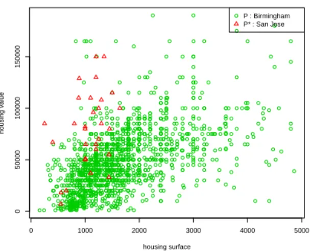
ad-0 1000 2000 3000 4000 5000 0 50000 100000 150000 housing surface housing v alue P : Birmingham P* : San Jose
Figure 1: Housing value vs surface for Birming-ham (AL, USA) and San Jose (CA, USA)
dition, to avoid the problem of numerous miss-ing values in the fourth class (for instance one third of the owners do not answer the question ”Is there a problem with crime in the neighbor-hood”), proxy variables have been used to take into account the quality of neighborhood with con-trol for the segmentation of the market (personal income, household size, number of cars owned). Finally, in this provisional treatment, a simple specification is used (no quadratic terms and no crossed effects). A more complex specification or mixes of several types of specifications constitute directions for future work. The difference between houses in Birmingham and San Jose is illustrated by Figure 1 which presents the value of the houses according to their surfaces.
The present work will show how a regression model of the house value estimated for the city of Birmingham can be adapted to the prediction of the houses values in San Jose.
2.2 The CO2-GNP dataset
Economic aspects of diffusion of greenhouse gases and their impact on environment play an impor-tant role on the countries economies, and their analysis have attracted a great interest in the last twenty years [2, 8]. As pointed out by [9], the study of such data could also be useful for coun-tries with low GNP in order to clarify in which development path they are embarking.
The objectives of this study is to investigate the relationship and causality between gross national
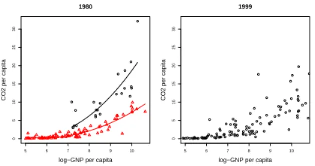
5 6 7 8 9 10 0 5 10 15 20 25 30 1980
log−GNP per capita
CO2 per capita
5 6 7 8 9 10 0 5 10 15 20 25 30 1999
log−GNP per capita
CO2 per capita
Figure 2: Emissions of CO2 per capita versus
GNP per capita in 1980 (left) and 1999 (right).
emissions to help current debates about emission projections. This study will also aim to determine typical economical politics of countries regarding
the environment. For this, the second dataset
studied in the present paper contains the CO2
emission per capita and the gross national prod-uct per capita, for 111 countries in 1980 and 1999. The sources of the data are The official United Na-tions site for the Millennium Development Goals
Indicators and the World Development Indicators
of the World Bank. Figure 2 plots the CO2
emis-sion per capita versus the logarithm of GNP per capita for 111 countries, in 1980 (left) and 1999 (right).
This paper will show on this dataset how the use of the 1980’s data can be helpful in the analy-sis of 1999’s data, by improving the quality of the regression models used to explain the relationship
between the gross national product and the CO2
emissions. Moreover, our analysis will allow to give information about the evolution of this rela-tionship from 1980 to 1999, and then to explain the economical political choices of particular coun-tries.
3
Adaptive models in regression
In this work, the adaptive regression models pro-posed in [4] and [5] will be used to analyze and understand the population evolution of the two datasets presented in the previous section. This section briefly reviews these adaptive regression models.
3.1 Adaptive linear models
The general setting of regression analysis is to identify a relationship (the regression model)
be-tween a response variable and one or several ex-planatory variables. Adaptive linear models have been defined in order to adapt an existing regres-sion model to a new situation, in which the vari-ables are identical but with a possible different probability density distribution and the relation-ship between response and explanatory variables could have changed.
Linear models for regression In regression
analysis, the data S = {(x1, y1), ..., (xn, yn)}
which arise from a population P , are assumed to be independent and identically distributed sam-ples from an unknown distribution, where x =
(x(1), . . . , x(p)) ∈ Rp and Y ∈ R. In regression
studies, Y is considered as a stochastic variable
and x as a deterministic one. A general data
modeling problem is to identify the relationship between the explanatory variable x (or covari-ate) and the response variable Y (or dependent
variable). Both standard parametric and
non-parametric regression approaches start with the following model:
Y = f (x, β) + ǫ, (1)
with ǫ ∼ N (0, σ2) and where β is a vector of real
regression parameters. The most common model is the linear form:
f(x, β) = β0+
d
X
i=1
βiψi(x), (2)
with β = (β0, β1, . . . , βd) ∈ Rd+1 are the
regres-sion parameters, and (ψi)1≤i≤dis a basis of
sion functions. In particular, usual linear
regres-sion occurs when d = p and ψi(x) = x(i).
How to adapt a regression model to another
population? Let us assume that the estimation
of the regression function f has been obtained in a preliminary study by using the sample S, and that a new regression model has to be adjusted
on a new sample S∗ = {(x∗
1, y1∗), ..., (x∗n∗, y∗n∗)},
measured on the same variables but arising from
another population P∗ (n∗is generally assumed to
be small). The new regression model on P∗ can
be written: Y|x∗ ∼ N (f (x∗, β∗), σ2), with f(x∗, β∗) = β∗ 0 + d X i=1 βi∗ψi(x∗).
Let us now precise the focus of adaptive linear models by making the two following assumptions.
Firstly, the variables (Y, x) and (Y∗, x∗) are
as-sumed to be the same but measured on two
differ-ent populations. Secondly, the size n∗ of the
ob-servation sample S∗ = (y∗
i, x∗i)i=1,n∗ of population
P∗ is assumed to be small compared to the
num-ber of observations of the reference population P . Otherwise, the mixture regression model could be estimated directly without using the training pop-ulation.
We consider the following transformation model between both regression functions for modeling the link between both populations:
f(x∗, β∗) = φ(f (x, β)). (3)
Since the transformation model (3) proposed in the previous section is a very general model, we propose to assume that the transformation func-tion φ has the following form:
φ(f (x, β)) = f (x, λβ)
with λ ∈ Rd+1. This transformation can be also
written in term of the regression parameters of both models as follows:
βi∗= λiβi ∀i = 1, . . . , d, (4)
with λi ∈ R. Let us also notice that the
regres-sion functions ψi are assumed to be the same for
both regression models, which is natural since the variables are identical in both populations.
A family of transformation models As the
number of parameters to estimate for the transfor-mation (4) is equal to (d + 1), learning this trans-formation model is equivalent to learn a new
re-gression model from the sample S∗. It is therefore
necessary to reduce the number of free parameters and that can be done by imposing constraints on
the transformation parameters λi. Then, a family
of 7 transformation models is considered, named further Adaptive Linear Models, from the most
complex model (hereafter M0) to the simplest one
(hereafter M6):
• Model M0: β∗0 = λ0β0 and βi∗ = λiβi, for
i= 1, ..., d. This model is the most complex
model of transformation between both
popu-lations P and P∗, and is equivalent to
learn-ing a new regression model from the
sam-ple S∗.
• Model M1: β0∗ = β0 and βi∗ = λiβi for i =
1, ..., d. This transformation model assumes that both regression models have the same
intercept β0.
• Model M2: β0∗ = λ0β0 and βi∗ = λβi for
i = 1, ..., d. This transformation model
as-sumes that the intercept of both regression
models differ by the scalar λ0 and all the
other regression parameters differ by the same scalar λ.
• Model M3: β∗0 = λβ0 and βi∗ = λβi for
i = 1, ..., d. This transformation model
as-sumes that all the regression parameters of both regression models differ by the same scalar λ.
• Model M4: β0∗ = β0 and βi∗ = λβi for
i = 1, ..., d. This transformation model
as-sumes that both regression models have the
same intercept β0and all the other regression
parameters differ by the same scalar λ.
• Model M5: β0∗ = λ0β0 and βi∗ = βi for i =
1, ..., d. This transformation model assumes that both regression models have the same parameters except the intercept.
• Model M6: β0∗ = β0 and βi∗ = βi for i =
1, ..., d. This model assume that both
popu-lations P and P∗ have the same behavior.
The numbers of parameters to estimate for these transformation models are presented in Table 2. Remark that it is possible to consider interme-diate models, by imposing specific constraints on
some parameters λi for given i ∈ {1, . . . , d}. The
practician could use his experimental knowledge to introduce some intermediate models especially useful for his application.
Estimation procedure and model selection The estimation procedure is made of two main steps corresponding to the estimation of the re-gression parameters on the population P and the estimation of the transformation parameters using
samples of the population P∗. The natural way for
the first estimation step is to use the ordinary least squares (OLS) procedure. Once the regression pa-rameters of population P have been learned, the parameters of the transformation models can also be estimated using the OLS procedure. However, by lack of space, the corresponding estimators are
Model M0 M1 M2 M3 M4 M5 M6
Parameters numbers d+1 d 2 1 1 1 0
Table 1: Complexity (number of parameters) of the transformation models. We recall that the models
M0 and M6 correspond respectively to OLS on P∗ and OLS on P .
not presented in this paper but can be found in [4]. Finally, the cross validation PRESS criterion [1] is used in order to select the most appropriate model for the data among the 7 Adaptive Linear Models.
3.2 Adaptive mixture models
As an alternative to linear models for modeling complex systems, the mixture of regressions is a popular approach which has been introduced by [7] as the switching regression model. In par-ticular, this model is often used in Economics for modeling phenomena with different phases. It as-sumes that the dependent variable Y ∈ R can be
linked to a covariate x = (1, x(1), ..., x(p)) ∈ Rp+1
by one of K possible regression models:
Y = xtβk+ σkε, k= 1, ..., K (5)
where ε ∼ N (0, 1), βk = (βk0, ..., βkp) ∈
{β1, . . . , βK} is the regression parameter vector
in Rp+1and σ2k∈ {σ2
1, . . . , σK2 } is the residual
vari-ance. The conditional density distribution of Y given x is therefore: p(y|x) = K X k=1 πkφ(y|xtβk, σk2), (6)
where π1, ..., πK are the mixing proportions (with
the classical constraint PKi=1πk = 1), and
φ(·|xtβ
k, σk2) is the Gaussian density parametrized
by its mean xtβ
k and variance σ2k. As for the
adaptive linear models, the new population P∗,
for which we want to predict Y , is assumed to be different from the training population P . The
mixture regression model for P∗ can be written as
follows: Y∗ = x∗tβ∗ k+ σ ∗ kε ∗ p(y∗|x∗) = K∗ X k=1 πk∗φ(y∗|x∗tβ∗ k, σ∗k2) (7) with ε∗ ∼ N (0, 1), β∗ k ∈ {β1∗, . . . , βK∗∗} and σ ∗ k ∈ {σ∗
1, . . . , σ∗K∗}. In addition to the assumptions
made in the previous section, as both populations have the same nature, each mixture is assumed to
have the same number of components (K∗ = K).
Under these assumptions, the goal is then to
pre-dict Y∗ for some new x∗ by using both samples
S= (yi, xi)i=1,n and S∗.
A family of transformation models
Follow-ing the strategy of the linear case, the general transformation model is considered:
βk∗ = Λkβk, (8)
where Λk= diag(λk0, λk1, . . . , λkp)
σk∗ is free,
where diag(λk0, λk1, . . . , λkp) is the diagonal
ma-trix containing (λk0, λk1, . . . , λkp) on its diagonal
completed by zeros. The family of parsimonious models is defined by imposing some constraints
on Λk:
• M M1 assumes that both populations are the
same population: Λk= Idis the identity
ma-trix,
• M M2 assumes that the link between
popu-lations is covariate and mixture component independent: – M M2a : λk0 = 1, λkj = λ and σk∗ = λσk ∀1 ≤ j ≤ p, – M M2b : λk0 = λ, λkj = 1 and σk∗ = σk ∀1 ≤ j ≤ p, – M M2c : Λk = λIdand σ∗k= λσk, – M M2d : λk0 = λ0, λkj = λ1 and σk∗ = λ1σk ∀1 ≤ j ≤ p,
• M M3 assumes that the link between
popula-tions is covariate independent:
– M M3a : λk0 = 1, λkj = λk and σk∗ = λkσk ∀1 ≤ j ≤ p, – M M3b : λk0 = λk, λkj = 1 and σk∗ = σk ∀1 ≤ j ≤ p, – M M3c : Λk = λkId and σk∗ = λkσk, – M M3d : λk0 = λk0, λkj = λk1 and σ∗k= λk1σk ∀1 ≤ j ≤ p,
• M M4 assumes that the link between
popula-tions is mixture component independent:
– M M4a : λk0 = 1 and λkj =
λj ∀1 ≤ j ≤ p,
– M M4b : Λk = Λ with Λ a diagonal
ma-trix,
• M M5 assumes that Λk is unconstrained,
which leads to estimate the mixture
regres-sion model for P∗ by using only S∗.
Moreover, the mixing proportions are allowed to be the same in each population or to be different
between both populations P and P∗. In the latter
case, they consequently have to be estimated using
the sample S∗. Corresponding notations for the
models are respectively M M· and pM M·. Table 2
gives the number of parameters to estimate for each model. If the mixing proportions are different
from P to P∗, K − 1 parameters to estimate must
be added to these values.
Estimation procedure and model selection As before, the estimation procedure is made of two steps. The first step consists in estimating model parameters for the reference population P whereas the second one focuses on the estimation of the link parameters. The estimation of the mixture
re-gression parameters β∗
k are deduced afterward by
plug-in. Conversely to the case of linear models, parameter estimation can not be done with the standard OLS procedure and the estimation has to be carried out by maximum likelihood using a missing data approach via the EM algorithm [6]. Estimation details can be found in [5]. Finally, in order to select among the transformation mod-els previously defined the most appropriate model of transformation between the populations P and
P∗, we propose to use the PRESS criterion [1] or
the Bayesian Information Criterion (BIC, [11]).
4
Experimental results
The two adaptive strategies reviewed in the previ-ous will be now applied to the AHS and CO2/GNP datasets.
4.1 The housing market data
A semi-log regression model for the housing mar-ket of Birmingham was learned using all the 1541 available samples and, then, the 7 adaptive linear
20 40 60 80 100 6 7 8 9 10
Size of training dataset
log(MSE) Model M0 Model M1 Model M2 Model M3 Model M4 Model M5 Model M6
Figure 3: MSE results for the Birmingham-San Jose data. 20 40 60 80 100 −2 −1 0 1 2
Size of training dataset
log(PRESS) Model M0 Model M1 Model M2 Model M3 Model M4 Model M5
Figure 4: PRESS criterion for the Birmingham-San Jose data.
models were used to transfer the regression model of Birmingham to the housing market of San Jose. In order to evaluate the ability of the adaptive lin-ear models to transfer the Birmingham knowledge to San Jose in different situations, the experiment protocol was applied for different sizes of San Jose samples ranging from 5 to 921 observations. For each dataset size, the San Jose samples were ran-domly selected among all available samples and the experiment was repeated 50 times for averag-ing the results. For each adaptive linear model, the PRESS criterion and the mean squard error (MSE) were computed, by using the selected sam-ple for PRESS and the whole San Jose dataset for MSE.
Figure 3 shows the logarithm of the MSE for the different adaptive linear models regarding to the
Model M M1 M M2a−c M M2d M M3a−c M M3d M M4a M M4b M M5
Param. 0 1 2 K 2K p+ K p+ K + 1 K(p + 2)
Table 2: Number of parameters to estimate for each model of the proposed family.
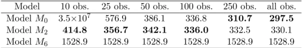
Model 10 obs. 25 obs. 50 obs. 100 obs. 250 obs. all obs.
Model M0 3.5×10⁷ 576.9 386.1 336.8 310.7 297.5
Model M2 414.8 356.7 342.1 336.0 332.5 330.1
Model M6 1528.9 1528.9 1528.9 1528.9 1528.9 1528.9
Table 3: MSE results for the Birmingham-San Jose data. size of the used San Jose samples. Similarly,
Fig-ure 4 shows the logarithm of the PRESS criterion.
Firstly, Figure 3 indicates that the model M6,
which corresponds to the Birmingham’s model, is actually not adapted for modeling the housing market of San Jose since it obtains a not satis-fying MSE value. Let us notice that the curve
corresponding to the MSE of the model M6 is
con-stant since the regression model has been learned on the Birmingham’s data and consequently does not depend on the size of the San Jose’s dataset
se-lected for learning. Secondly, the model M0, which
is equivalent to OLS on the San Jose samples, is particularly disappointing (large values of MSE) if learned with a very small number of observations and becomes more efficient for learning datasets
larger than 50 observations. The model M1 has
a similar behavior for small learning datasets but
turns out to be less interesting than M0 when the
size of the learning dataset is larger. These
behav-iors are not surprising since both models M0 and
M1 are very complex models and then need large
datasets to be correctly learned. Conversely, the
models M2to M5appear not to be sensitive to the
size of the dataset used for adapting the
Birming-ham model. Particularly, the model M2 obtains
very low MSE values for a learning dataset size as low as 20 observations. This indicates that the
model M2 is able to adapt the Birmingham model
to San Jose with only 20 observations. Moreover,
Table 3 indicates that the model M2 provides
bet-ter prediction results than the model M0 for the
housing market of San Jose for learning dataset sizes less than 100 observations. Naturally, since
the model M0 is more complex, it becomes more
efficient than the model M2 for larger datasets
even though the difference is not so big for large learning datasets. Figure 4 shows that the PRESS criterion, which will be used in practice since it is computed without a validation dataset, allows the
practician to successfully select the most appro-priated transfer model. Indeed, it appears clearly that the PRESS curves are very similar to the MSE curves computed on the whole dataset. Fi-nally, in such a context, the transformation pa-rameters obtained by the different adaptive linear models can be interpreted in an economic way and this could be interesting for economists. In partic-ular, the estimated transformation parameters by
the model M2 with the whole San Jose dataset are
λ0 = 1.439 and λ = 0.447. The results obtained,
mainly a proportionality between the parameters, suggest that, in this case, the contribution of each characteristic to the growth of the housing value in the second city is just one half of what it is in the first one, while, in the same time, the ba-sic price in the second city is one time and a half greater. This results from a simple regulation pro-duced by the market, if the constraint of the same specification for the two cities is validated by the statistical results. In terms of MSE and PRESS we obtain good indicators of the validation of this constraint within the scope defined for this initial approach.
To summarize, this experiment has shown that the adaptive linear models are able to transfer the knowledge on the housing market of a reference city to the market of a different city with a small number of observations. Furthermore, the inter-pretation of the estimated transformation param-eters could help the practician to analyze in an economic way the differences between the studied populations.
4.2 The CO2-GNP data
A mixture of second order polynomial regressions seems to be particularly well adapted to fit the link
between the CO2 emissions and the log-GNP, and
30% of the 1999’s data (n∗= 33)
model BIC PRESS MSE
pM M2a 13.21 4.01 4.77 pM M2b 12.89 4.57 3.66 pM M2c 12.57 4.16 4.55 pM M2d 17.13 4.38 4.77 pM M3a 15.92 4.49 4.66 pM M3b 16.01 5.59 4.11 pM M3c 15.75 6.17 4.23 pM M3d 22.72 4.49 4.66 UR 27.08 7.46 7.66 MR 32.89 5.54 5.11 50% of the 1999’s data (n∗= 55)
model BIC PRESS MSE
pM M2a 14.10 4.76 3.88 pM M2b 13.99 4.10 3.77 pM M2c 14.07 5.29 4.22 pM M2d 17.82 4.45 4.66 pM M3a 18.07 4.27 4.66 pM M3b 18.00 5.62 4.44 pM M3c 17.60 5.62 4.33 pM M3d 26.61 6.12 4.55 UR 20.87 7.95 7.21 MR 39.69 4.82 4.77 70% of the 1999’s data (n∗= 77)
model BIC PRESS MSE
pM m2a 15.15 5.51 8.21 pM M2b 14.82 3.89 3.77 pM M2c 14.71 4.53 4.44 pM M2d 19.00 5.83 4.99 pM M3a 18.96 4.79 4.44 pM M3b 19.06 4.34 4.22 pM M3c 18.98 5.26 3.77 pM M3d 27.57 5.55 4.88 UR 22.08 8.00 7.10 MR 43.91 5.06 3.33 (n∗= 111)
model BIC PRESS MSE
pM M2a 15.51 3.83 3.77 pM M2b 15.54 3.87 4.77 pM M2c 15.34 4.13 4.11 pM M2d 20.14 4.41 4.33 pM M3a 20.19 4.48 4.77 pM M3b 20.03 4.41 4.33 pM M3c 20.06 4.35 3.44 pM M3d 29.55 4.76 5.44 UR 23.62 7.53 6.99 MR 47.19 3.66 2.89
Table 4: MSE on the whole 1999’s sample, PRESS and BIC criterion for the 8 adaptive mixture
models (pM M2a to pM M3d), usual regression model (UR) and classical regressions mixture model
(MR), for 4 sizes of the 1999’s sample: 33, 55, 77 and 111 (whole sample). Lower BIC, PRESS and MSE values for each sample size are in bold character.
5 6 7 8 9 10 0 5 10 15 20 25 30 35 1980
log−GNP per capita
CO2 per capita
Algeria Antigua_and_Barbuda Argentina Australia Austria Bangladesh Barbados Belgium Belize Benin Bhutan Bolivia Botswana Brazil Bulgaria Burkina_Faso Burundi Cameroon Canada Central_African_Republic Chad Chile China Colombia ComorosCongo._Rep. Costa_Rica Cote_d’Ivoire Cyprus Dominica Dominican_Republic Ecuador Egypt._Arab_Rep. El_Salvador Fiji Finland France French_Polynesia Gabon Gambia._TheGhana Greece Grenada Guatemala Guinea−Bissau Guyana Haiti Honduras Hungary Iceland India Indonesia Iran._Islamic_Rep.
IrelandIsraelItaly
Jamaica Japan Jordan Kenya Korea._Rep. Luxembourg Madagascar Malawi Malaysia Mali Malta Mauritania Mauritius Mexico Morocco MozambiqueNepal Netherlands New_Caledonia Nicaragua Niger Nigeria Norway Pakistan Panama Papua_New_Guinea Paraguay Peru Philippines Portugal Romania Rwanda Saudi_Arabia Senegal Seychelles Sierra_Leone Singapore Solomon_Islands South_Africa Spain Sri_Lanka Swaziland Sweden Switzerland Syrian_Arab_Republic Thailand Togo Trinidad_and_Tobago TunisiaTurkey United_States Uruguay Venezuela._RB Zambia Zimbabwe 5 6 7 8 9 10 11 0 5 10 15 20 25 30 35 1999
log−GNP per capita
CO2 per capita
Algeria Antigua_and_Barbuda Argentina Australia Austria Bangladesh Barbados Belgium Belize BeninBhutan Bolivia BotswanaBrazil Bulgaria Burkina_Faso Burundi Cameroon Canada Central_African_RepublicChad Chile China Colombia ComorosCongo._Rep. Costa_Rica Cote_d’Ivoire Cyprus Dominica Dominican_Republic Ecuador Egypt._Arab_Rep. El_SalvadorFiji Finland France French_Polynesia Gabon Gambia._TheGhana Greece Grenada Guatemala Guinea−Bissau Guyana Haiti Honduras Hungary Iceland India Indonesia Iran._Islamic_Rep. Ireland Israel Italy Jamaica Japan Jordan Kenya Korea._Rep. Luxembourg Madagascar Malawi Malaysia Mali Malta Mauritania Mauritius Mexico Morocco MozambiqueNepal Netherlands New_Caledonia Nicaragua NigerNigeria Norway Pakistan Panama Papua_New_GuineaParaguay Peru Philippines Portugal Romania Rwanda Saudi_Arabia Senegal Seychelles Sierra_Leone Singapore Solomon_Islands South_Africa Spain Sri_Lanka Swaziland SwedenSwitzerland Syrian_Arab_Republic Thailand Togo Trinidad_and_Tobago Tunisia Turkey United_States Uruguay Venezuela._RB Zambia Zimbabwe
Figure 5: Emissions of CO2 per capita versus GNP per capita in 1980 (left) and 1999 (right) and
two groups of countries are easily distinguishable: a first minority group (about 25% of the whole sample) is made of countries for which a grow
in the GNP is linked to a high grow of the CO2
emission, whereas the second group (about 75%) seems to have more environmental political orien-tations. This country discrimination in two groups is more difficult to obtain on the 1999’s data: it seems (from Figure 2) that countries which had
high CO2 emission in 1980 have adopted a more
environmental development than in the past, and a two-component mixture regression model could be more difficult to exhibit.
In order to help this distinction, adaptive mix-ture models are used to estimate the mixmix-ture re-gression model on the 1999’s data. The eight
mod-els pM M2ato pM M3d (since pM M4a and pM M4b
are equivalent to pM M2a and pM M2c for p = 1),
classical mixture of second order polynomial re-gressions with two components (MR) and usual second order polynomial regression (UR) are con-sidered. Different sample size of the 1999’s data
are tested: 30%, 50%, 70% and 100% of the S∗size
(n∗ = 111). The experiments have been repeated
20 times in order to average the results. Table 4 summarizes these results: MSE corresponds to the mean square error, whereas PRESS and BIC are the model selection criteria introduced in Sec-tion 3. In this applicaSec-tion, the total number of available data in the 1999 population is not suf-ficiently large to separate them into two training and test samples. For this reason, MSE is
com-puted on the whole S∗ sample, although a part of
it has been used for the training (from 30% for the first experiment to 100% for the last one). Con-sequently, MSE is a significant indicator of pre-dictive ability of the model when 30% and 50% of the whole dataset are used as training set since 70% and 50% of the samples used to compute the MSE remain independent from the training stage. However, MSE is a less significant indicator of pre-dictive ability for the two last experiments and the PRESS should be preferred in these situations as indicator of predictive ability.
Table 4 first allows to remark that the 1999’s data are actually made of two components as in the 1980’s data since both PRESS and MSE are better for MR (2 components) than UR (1
com-ponent) for all sizes n∗ of S∗. This first result
validates the assumption that both the reference
population P and the new population P∗ have
the same number K = 2 components, and
conse-quently the use of adaptive mixture of regression does make sense for this data. Secondly, adaptive mixture models turns out to provide very
satis-fying predictions for all values of n∗ and
particu-larly outperforms the other approaches when n∗
is small. Indeed, both BIC, PRESS and MSE testify that these models provide better
predic-tions than the other studied methods when n∗ is
equal to 30%, 50% and 70% of the whole sample. Furthermore, it should be noticed that adaptive mixture model provide stable results according to
variations on n∗. In particular, the models pM M
2
are those which appear the most efficient on this dataset and this suggests that the link between
both populations P and P∗ is mixture component
independent. This application illustrates well the interest of combining informations on both past (1980) and present (1999) situations in order to
analyze the link between CO2 emissions and gross
national product for several countries in 1999, es-pecially when the number of data for the present situation is not sufficiently large. Moreover, the competition between the adaptive mixture mod-els is also informative. Indeed, it seems that three models are particularly well adapted to model the link between the 1980’s data and those of 1999’s
data: pM M2a, pM M2b and pM M2c. The
partic-ularity of these models is that they consider the same transformation for both classes of countries, which means that all the countries have the same kind of evolution.
The estimated mixture of two regression models on the 1980’s data is:
CO2 = 26.96 − 9.62 log(GN P ) + 0.88 log(GN P )2
CO2 = 13.42 − 4.57 log(GN P ) + 0.40 log(GN P )2
with respective probability π1 = 0.26 and π2 =
0.74 and residual variances σ12 = 3.10 and σ12 =
0.55. The model for the 1999’s data obtained with
model pM M2c (for the whole sample size) is
ob-tained with a link parameter λ = 1.26:
CO2 = 33.92 − 12.1 log(GN P ) + 1.11 log(GN P )2
CO2 = 16.89 − 5.75 log(GN P ) + 0.50 log(GN P )2
with π1 = 0.15, σ∗21 = 4.9, π2 = 0.85 and σ∗21 =
0.87.
These results are illustrated by Figure 5. One can first remark that there are still two groups of countries: the first group of countries has a low ratio CO2/GNP whereas the second one as a highest ratio. Without trying to generalize, the
presence of two types of countries may indicate the existence of two different environmental pol-itics. In particular, one can remark that USA, Canada and Australia remain in the group of high CO2/GNP ratio whereas Belgium, Netherlands, Finland and New Caledonia have moved from the high CO2/GNP group to the low CO2/GNP group.
This experiment are therefore shown that the use of adaptive models for switching regression can help the practician in understanding and inter-prating the evolution of the studied phenomenum.
5
Conclusion
When carrying out a regression analysis to analyze a phenomenon which have already been studied in different conditions, adaptive models can help to exploit the previous analysis in order to emphasize the quality of the current one. In this paper, we have shown how a regression model predicting the house value can be adapted from the US South-East to the US West coast, and how the regression
of the CO2 emissions in function to the gross
na-tional product in 1999 can be estimated by using information about the same analysis in 1980. In such contexts, the adaptive models proposed in [4] and [5] can help the practician in both improving the prediction quality and for understanding the evolution of the studied phenomenon. Let us fi-nally notice that similar models exist in a classifi-cation context [3, 10] as well and allow to classify observations in a situation different from the one in which the classification rule has been estimated.
References
[1] D. M. Allen. The relationship between vari-able selection and data augmentation and
a method for prediction. Technometrics,
16:125–127, 1974.
[2] T. Barker. Measuring economic costs of co2
emission limits. Energy, 16(3):611 – 614,
1991.
[3] C. Biernacki, F. Beninel, and V. Bretag-nolle. A generalized discriminant rule when training population and test population differ on their descriptive parameters. Biometrics, 58(2):387–397, 2002.
[4] C. Bouveyron and J. Jacques. Adaptive lin-ear models for regression: improving predic-tion when populapredic-tion has changed. Pattern Recognition Letters, 31(14):2237–2247, 2010. [5] C. Bouveyron and J. Jacques. Adaptive
mix-tures of regressions: Improving predictive in-ference when population has changed. Pub. IRMA Lille, 70(8), 2010.
[6] A.P. Dempster, N.M. Laird, and D.B. Ru-bin. Maximum likelihood from incomplete data (with discussion). Journal of the Royal Statistical Society. Series B, 39:1–38, 1977. [7] M. Goldfeld and R.E. Quandt. A markov
model for switching regressions. Journal of Econometrics, 1:3–16, 1973.
[8] M. Grubb et al. Ha-Duong, M. Influence
of socio-economic inertia and uncertainty on
optimal co2-emission abatement. Nature,
390:170–173, 1997.
[9] M. Hurn, A. Justel, and C. Robert. Estimat-ing mixtures of regressions. Journal of Com-putational and Graphical Statistics, 12(1):55– 79, 2003.
[10] J. Jacques and C. Biernacki. Extension
of model-based classification for binary data when training and test populations differ. Journal of Applied Statistics, 37(5):749–766, 2010.
[11] G. Schwarz. Estimating the dimension of a model. Ann. Statist., 6(2):461–464, 1978.