Final-Year Project (TN10)
Internship Report
Controlling processing consistency, quality
and efficiency by predictive modeling of meat
by-products transformation
INRA Centre of Theix (Auvergne, France)
AgResearch Centre of Lincoln (Canterbury, New Zealand)
LEPERS Valentin Process Engineering Student February 16th 2015 – July 31st 2015
UTC Supervisor : Pr Khalil SHAKOURZADEH BOLOURI INRA Supervisor : Dr Alain KONDJOYAN AgResearch Supervisor : Dr Stefan CLERENS
2
Résumé technique
En Nouvelle-Zélande, Taranaki Bio Extracts (TBE), filiale du groupe ANZCO a mis au point un procédé d'extraction de protéines depuis les co-produits de l'industrie de la viande. Ainsi, des carcasses de boeuf sont amenées à haute température dans un milieu aqueux sous pression afin d'en extraire les protéines structurelles (principalement du collagène de type I). Afin de mieux comprendre les phénomènes intervenant au cours du procédé, un contrat a été établi entre TBE et AgResearch, le principal institut de recherche néo-zélandais. Le centre INRA de Theix (région Auvergne) a rejoint le projet en raison des compétences en modélisation dont il disposait.
Des expériences en laboratoire ont été réalisées à AgResearch (cuisson sous pression et à différentes températures d'os de bœuf et de viande grasse présente sur les carcasses) afin de déterminer les cinétiques d'extraction protéique au cours du procédé, l'évolution colorimétrique du bouillon (paramètre critique du produit final) et, dans une moindre mesure, la composition des produits obtenus à l'échelle moléculaire. Les résultats ont été interprétés et exploités à l'INRA.
Mots-clés : Recherche, International, Agro-industrie, Procédé, Laboratoire, Viande, Os, Biologie, Biochimie, Protéines
3
Acknowledgements
Before starting the actual report of my 24 weeks spent between Auvergne in France and Canterbury in New Zealand, I would sincerely like to thank all the people that helped me at some point during this project :
My two supervisors : Dr Alain Kondjoyan at INRA and Dr Stefan Clerens at AgResearch for their trust, their receptiveness, their sympathy and their benevolence. Having the opportunity to discover Research and to travel to New Zealand at the same time was truly special.
Dr Santanu Deb-Choudhury, one of my coworkers at AgResearch, for his receptiveness, his patience, and his daily good mood and sense of humor.
Mike North, the plant manager of TBE III, for his nice welcome and for having taken the time to walk us through his process when Dr Deb-Choudhury and I visited him in Hawera.
4
Table of Contents
Résumé technique ... 2 Acknowledgements ... 3 Table of illustrations ... 6 Tables ... 6 Figures ... 6 Introduction ... 8 I/ Internship context ... 9 I ; 1/ Presentation of INRA ... 9 I ; 2/ Presentation of AgResearch ... 10I ; 3/ Presentation of Taranaki Bio Extracts ... 11
II/ Project problematization ... 12
II ; 1/ Raw material composition ... 12
II ; 2/ Process description ... 14
II ; 3/ Involved phenomena ... 17
III/ Material and methods ... 19
III ; 1/ Experimental design ... 19
III ; 1 ; 1/ Preliminary reflection ... 19
III ; 1 ; 2/ Building the definitive experimental design ... 20
III ; 2/ Analysis methods ... 22
III ; 3/ Experimental raw material preparation ... 26
III ; 4/ Design and working of the lab scale pressure cooker ... 27
IV/ Results, analysis and discussion... 32
IV ; 1/ Modification of the experimental set-up ... 32
IV ; 1 ; 1/ Beef meat and scraps early results : first two runs in AgResearch’s pressure cooker ... 32
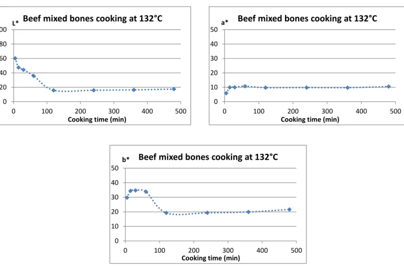
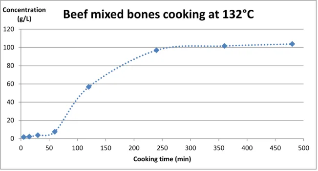
IV ; 1 ; 2/ Beef mixed bones early results : highlighting a mixing defect ... 35
IV ; 1 ; 3/ Improving the pressure cooker ... 37
IV ; 2/ Measurement uncertainties ... 39
IV ; 2 ; 1/ Colour measurement ... 39
IV ; 2 ; 2/ Protein concentration measurement ... 40
IV ; 3/ Final experimental results ... 42
IV ; 3 ; 1/ Colour measurements ... 43
5
IV ; 3 ; 3/ Amino acid analysis ... 54
IV ; 3 ; 4/ Mass spectrometry results... 56
IV ; 4/ Modeling and analysis ... 59
IV ; 4 ; 1/ Heat transfer modeling ... 59
IV ; 4 ; 2/ Proteins extraction kinetics modeling ... 62
IV ; 5/ Prospects for TBE ... 67
Conclusion ... 69
References ... 70
Annex ... 72
Annex 1 : Colour evolution of stocks ... 72
Beef scraps ... 72
Leg bones (130°C) ... 73
Mixed bones ... 73
Annex 2 : Cooked material pictures ... 74
Beef scraps ... 74
Leg bones (130°C) ... 74
6
Table of illustrations
Tables
Table 1 : Bone material composition (Composition de la matière osseuse) ... 13
Table 2 : Beef scraps composition (Composition des déchets) ... 13
Table 3 : Raw material composition (Composition de la matière première) ... 13
Table 4 : Experimental raw material composition (Composition de la matière première utilisée en laboratoire) ... 26
Table 5 : 90°C uncertainty measurement (Mesure des incertitudes à 90°C) ... 41
Table 6 : 110°C/130°C uncertainty measurement (Mesure des incertitudes à 110°C/130°C) ... 42
Table 7 : Final runs working conditions (Conditions de fonctionnement des runs finaux) ... 43
Table 8 : Beef scraps cooking : T-P evolution (Cuisson de déchets : évolution de T et P) ... 49
Table 9 : Beef scraps cooking : achieved extraction yelds (final results) (Cuisson de déchets : rendements d’extraction obtenus, résultats finaux) ... 50
Table 10 : Beef leg bones cooking at 130°C : T-P evolution (Cuisson d’os de pattes de bœuf à 130°C : évolution de T et P) ... 51
Table 11 : Beef leg bones cooking at 130°C : achieved extraction yields (final results) (Cuisson d’os de pattes de bœuf à 130°C : rendements d’extraction obtenus, résultats finaux) ... 51
Table 12 : Beef mixed bones cooking : T-P evolution (Cuisson d’os de bœuf mélangés : évolution de T et P) ... 53
Table 13 : Beef mixed bones cooking : achieved extraction yields (final results) (Cuisson d’os de bœuf mélangés : rendements d’extraction obtenus, résultats finaux) ... 53
Table 14 : Amino acid analysis results (Résultats des analyses en acides aminés) ... 55
Table 15 : List of amino acid targets used for modification searches (Liste des acides amines ciblés par les recherches de modifications) ... 57
Table 16 : Heat transfer modeling : input parameters (Modélisation du transfert de chaleur : paramètres d’entrée) .... 61
Table 17 : Protein extraction tendencies, depending on cooking temperature and kind of raw material (Tendances de l’extraction protéique en fonction de la température du cuiseur et de la matière première) ... 63
Table 18 : Building the model : optimized parameters (Construction du modèle : paramètres optimisés) ... 64
Table 19 : Input values for the calculation of kinetics constants (Paramètres d’entrée pour le calcul des constantes de cinétique)... 66
Figures
Fig. 1 : Beef bone protein extraction process flow diagram (Flow chart du procédé d’extraction protéique sur des os de bœuf) __________________________________________________________________________________________ 16 Fig. 2 : First order kinetics curve (focusing on product) (Courbe typique de la cinétique de premier ordre) __________ 20 Fig. 3 : Meat and mixed bones cooking in an 85°C water bath : protein concentration (Cuisson de viande maigre et d’os mélangés dans un bain-marie à 85°C : concentration en protéines) _________________________________________ 21 Fig. 4 : CIE L*a*b* colour space (Représentation spatiale du modèle CIE L*a*b*) ______________________________ 23 Fig. 5 : Direct Detect spectrometer (Spectromètre Direct Detect) ___________________________________________ 24 Fig. 6 : AgResearch’s bone crushing equipment (Matériel utilisé par AgResearch pour le broyage des os) __________ 27 Fig. 7 : Assembled cooker, front view (Cuiseur assemblé, vue de face) _______________________________________ 28 Fig. 8 : Experimental cooker parameters control (Contrôle des paramètres du cuiseur expérimental) ______________ 29 Fig. 9 : Empty cooker, top view (Cuiseur vide, vue de dessus) ______________________________________________ 30 Fig. 10 : Cooker with basket, top view (Cuiseur avec panier, vue de dessus) __________________________________ 30 Fig. 11 : Cooking basket, side view (Panier de cuisson, vue de côté) _________________________________________ 30 Fig. 12 : Cooking basket, bottom view (Panier de cuisson, vue de dessous) ___________________________________ 30
7 Fig. 13 : Cooking basket, looking up inner tube. Arrows indicate rows of 5 mm diameter holes (Panier de cuisson, intérieur du tube) _________________________________________________________________________________ 31 Fig. 14 : Cooking basket, looking along inner tube (Panier de cuisson, extérieur du tube) ________________________ 31 Fig. 15 : Beef meat cooking at 132°C : colour evolution (early results) (Cuisson de viande de bœuf maigre à 132°C : évolution de la couleur, résultats préliminaires)_________________________________________________________ 33 Fig. 16 : Beef scraps cooking at 132°C : colour evolution (early results) (Cuisson de déchets à 132°C : évolution de la couleur, résultats préliminaires) _____________________________________________________________________ 33 Fig. 17 : Beef meat cooking at 132°C : protein concentration evolution (early results) (Cuisson de viande de bœuf maigre à 132°C : évolution de la concentration en protéines, résultats préliminaires) __________________________ 34 Fig. 18 : Beef scraps cooking at 132°C : protein concentration evolution (early results) (Cuisson de déchets à 132°C : évolution de la concentration en protéines, résultats préliminaires)_________________________________________ 34 Fig. 19 : Beef mixed bones cooking at 132°C : colour evolution (early results) (Cuisson d’os de bœuf mélangés à 132°C : évolution de la couleur, résultats préliminaires)_________________________________________________________ 35 Fig. 20 : Beef mixed bones cooking at 132°C : protein concentration evolution (early results) (Cuisson d’os de bœuf mélangés à 132°C : évolution de la concentration en protéines, résultats préliminaires) ________________________ 36 Fig. 21 : From left to right : scraps stock, lean meat stock and mixed bones stock after cooling, 8h mixed bones gel (early runs) (De gauche à droite : bouillons obtenus à partir de déchets, de viande maigre, et d’os mélangés après refroidissement, gel obtenu à partir d’os mélangés après 8h de cuisson (runs préliminaires) _____________________ 37 Fig. 22 : Pressure cooker with new motor, front view (Cuiseur avec moteur de remplacement, vue de face) _________ 38 Fig. 23 : Beef scraps cooking : colour evolution (final results) (Cuisson de déchets : évolution de la couleur, résultats finaux) _________________________________________________________________________________________ 44 Fig. 24 : Beef leg bones cooking at 130°C : colour evolution (final results) (Cuisson d’os de pattes de bœuf à 130°C : évolution de la couleur, résultats finaux) ______________________________________________________________ 45 Fig. 25 : Beef mixed bones cooking : colour evolution (final results) (Cuisson d’os de bœuf mélangés : évolution de la couleur, résultats finaux) ___________________________________________________________________________ 46 Fig. 26 : Beef scraps cooking : protein concentration evolution (final results) (Cuisson de déchets : évolution de la concentration en protéines, résultats finaux) ___________________________________________________________ 48 Fig. 27 : Beef leg bones cooking at 130°C : protein concentration evolution (final results) (Cuisson d’os de pattes de bœuf à 130°C : évolution de la concentration en protéines, résultats finaux) _________________________________ 50 Fig. 28 : Beef mixed bones cooking : protein concentration evolution (final results) (Cuisson d’os de bœuf mélangés : évolution de la concentration en protéines, résultats finaux) ______________________________________________ 52 Fig. 29 : Beef mixed bones cooking at 110°C and 130°C : oxidative modification scores (Cuisson d’os de bœuf mélangés à 110°C et 130°C : indices d’oxydation) _______________________________________________________________ 57 Fig. 30 : Beef mixed bones cooking at 110°C and 130°C : other modifications scores (Cuisson d’os de bœuf mélangés à 110°C et 130°C : autres indices de dégâts) _____________________________________________________________ 58 Fig. 31 : Lab scale heat transfer (central point) (Transfert de chaleur à l’échelle expérimentale, point central) _______ 61 Fig. 32 : Process scale heat transfer (central point) (Transfert de chaleur à l’échelle industrielle, point central) ______ 61 Fig. 33 : Process scale cooker temperature profile : t = 8h, y' = 0 (Profil de température du cuiseur industriel : t = 8h, y’ = 0) _____________________________________________________________________________________________ 62 Fig. 34 : Beef mixed bones cooking : protein extraction modeling (Cuisson d’os de bœuf mélangés : modélisation de l’extraction protéique) _____________________________________________________________________________ 64 Fig. 35 : Beef scraps cooking : protein extraction modeling (Cuisson de déchets : modélisation de l’extraction protéique) _______________________________________________________________________________________________ 65 Fig. 36 : Beef leg bones cooking : protein extraction modeling (Cuisson d’os de pattes de bœuf : modélisation de l’extraction protéique) _____________________________________________________________________________ 65
8
Introduction
Beef meat is nowadays an ordinary consumer product in most civilizations around the World and the current emergence of new economical powers results in a constantly higher demand for it. However, customers are only interested in precise parts of the animal (i.e. lean meat), while the rest (bones, connective tissues, residual meat… that represent 30% of the carcass mass) is at best considered as by-products and at worst as waste that needs to be removed from food by-products fabrication processes. When they are not destroyed, by-products can be sold, for example as an ingredient for broth or as pets food. Bones can also be used at industrial scale for gelatin or animal meal fabrication, among other things. However, the proportion of bones recovered through these processes is rather low.
If bones are used in this manner, this is because they display interesting nutritive properties as they are constituted by 65% of minerals and 35% of proteins (most of which is type I collagen, from which gelatin is a derived product). Bones as such represent about 50% of meat by-products, the rest being fat, residual meat, tendons and other connective tissues. Therefore, even with meat taken off, carcasses are a non-negligible source of proteins that need to be used, their destroying (via combustion) and burying being a potential cause of pollution and health risks. The process of animal meal seemed to provide a viable solution to this issue, but their use has been strictly regulated (if not forbidden) since the epidemic of bovine spongiform encephalitis (mad cow disease) that struck Europe during the 1990’s, making developing new carcass-based processes a necessity. Indeed, the worldwide demand for gelatin is far from being sufficient to absorb all bone waste, gelatin production processes moreover being time-consuming and providing low yields (in the 15-20 % range).
In New Zealand, Taranaki Bio Extracts (TBE), a 50:50 joint venture company between Taranaki By Products Ltd and ANZCO Foods Ltd, has developed a protein extraction process based on the hydrolysis of beef bones under high temperature and pressure, resulting in a protein-rich concentrated stock (bone extract). In 2014, TBE contacted AgResearch (the main New Zealand research institute) to establish a contract as they wanted a better understanding of the underlying phenomena that occurred during their process. AgResearch, on the other hand, contacted INRA in order to make the project international and to have available skills regarding modeling. A lab scale experimental set-up was built in AgResearch’s lab in Lincoln. During my final-year student project in Process Engineering (Université de Technologie de Compiègne, 16/02/2015 – 31/07/2015), I performed experiments in Lincoln before exploiting the results in Theix (INRA centre of Clermont-Ferrand). During this study, we focused on proteins extraction kinetics, stock colour evolution (colour being a critical property of the final product), and to a lesser extent, on the product composition at molecular scale. From these results, hypotheses were built regarding the extraction mechanisms (some of which were modeled) and proposals were made regarding process improvement. The results of this study are now being used for the writing of a scientific publication.
9
I/ Internship context
I ; 1/ Presentation of INRA
INRA (National Institute for Agricultural Research) is a French public research institute dedicated to scientific studies concerning agriculture. It was founded in 1946 and is a Public Scientific and Technical Research Establishment (EPST) under the joint authorities of Ministries of Research and Agriculture. Since April of 2012, the Institute has been presided by François Houllier. INRA leads projects of research for a sustainable agriculture, a safeguarded environment and a healthy and high quality food. Based on the number of publications in agricultural, crops and animal sciences, INRA is the first institute for agricultural research in Europe, and the second in the world. It belongs to the top 1% most cited research institutes and its main tasks are :
To gather and disseminate knowledge ;
To build know-how and innovation for the society ;
To provide expertise to public institutions and private companies ;
To participate in science-society debates ;
To train in research.
The institute employs roughly 1800 researchers, 2400 research engineers, 4200 lab workers/field workers/administrative staff. It also welcomes 1700 PhD students and 1000 interns/foreign researchers every year. INRA is composed of 13 scientific departments :
Environment and Agronomy ;
Biology and crop breeding ;
Plant health and environment ;
Ecology of forest, meadows and aquatic environment ;
Animal genetics ;
Animal physiology and animal production systems ;
Animal health ;
Characterization and processing of agricultural products ;
Microbiology and food processing ;
Human nutrition ;
Sciences for action and development ;
Social sciences, agriculture and food, territories and environment ;
Applied mathematics and computer science.
Nowadays, INRA has 17 regional centres in France, on more than 150 sites and it develops partnerships with Universities and French top-schools in agricultural/veterinary sciences, French research institutes of fundamental and targeted research (CNRS, INSERM), French research institues of agricultural applied research and the main agricultural research institutes in the world, nearly half of its publications being co-authored by non-French scientists. [1]
When I was working in France during my internship (16/02/2015 - 24/03/2015 ; 03/06/2015 - 31/07/2015), I was based at the centre of Clermont-Theix-Lyon, which employs research teams in Auvergne
10 and Rhône-Alpes regions as well as in Limoges. It is the third largest INRA research centre and it involves 8 % of the Institutes’ total staff, with almost all the previously listed scientific departments being represented there. The research team I was working in was part of the CEPIA department (Characterization and Processing of Agricultural Products), which studies the processing of animal/vegetal raw materials and waste (by-products, industrial and urban waste). The research led in this department is targeted on processing these raw materials into food products, materials (plastic…), energy or molecules for chemical and pharmaceutical industry. It employs 500 people, distributed among 23 laboratories on the French territory.
Each research department is divided into units and subunits. My team was part of the QuaPA (Quality of Animal Products) unit, led by Dr Alain Kondjoyan. The unit employs 36 people full-time, welcomes PhD and post-doc students on a regular basis and its purpose is to improve the safety and nutritional quality of animal products, while preserving their technological and sensory qualities. Lastly, I was working for the IT (Imaging and Transfer) team, whose purpose is to characterize the structural and chemical evolution of food products during their processing, but also during their digestion. Modeling is a major part of this team’s work.
I ; 2/ Presentation of AgResearch
AgResearch is New Zealand’s largest Crown Research Institute (CRI) and partners with the pastoral sector to identify and deliver the innovation that is needed to create value for the country. It employs approximately 850 staff spread across four campuses and farms in the Waikato, Manawatu, Canterbury and Otago regions. Agriculture is New Zealand’s largest export income earner, and AgResearch plays a key role in delivering new knowledge and technologies which underpin the pastoral, agri-food and agri-technology value chains. The institute is a leader in the following areas :
Pasture-based animal production systems ; New pasture plant varieties ;
Agriculture-derived greenhouse gas mitigation and pastoral climate change adaptation ; Agri-food and bio-based products and agri-technologies ;
Integrated social and biophysical research to support pastoral, agri-food and agri-technology sector development.
AgResearch’s science capability is divided into six groups :
Animal Productivity : the group encompasses a wide range of disciplines, with the purpose of developing advanced technology options for animal reproduction and enhancement of animal performance.
Food & Bio-based Products : its role is to create the knowledge and tools to develop high value foods, ingredients and products from pastoral-based agriculture. The group researches, develops and produces a diverse range of consumer materials from meat and dairy foods, woolen carpet and fabric, health and beauty products to the tools and machinery to support these industries.
Forage Improvements : the group develops new tools and technologies to improve on-farm productivity, enhance the performance of New Zealand’s pastoral, agricultural and biotechnology industries and build on New Zealand’s position at the forefront of these sectors.
11 Innovative Farm Systems : the group is committed to creating more profitable and sustainable
farms and agribusinesses.
Land and Environment : the group looks at land use and land management in relation to environmental impacts and climate change. Their goals are to improve dairy farming, beef, lamb and deer production systems by producing innovative research on soil and water management, pasture fertilization and farm nutrient management, while reducing negative impacts on the quality of soil, water and atmosphere and ecosystems.
Knowledge and Analytics : the group works very closely with researchers in meeting their knowledge and information resources needs. It also collaborates with internal and external scientists in providing data analysis solutions.[2][3]
When I was working in New Zealand during my internship (30/03/2015 - 27/05/2015), I was based at the Lincoln centre, 15 km West of Christchurch (Canterbury region). The research led in this centre focuses on biocontrol and biosecurity, plant breeding and seed technology, wool and skin biology and animal fibers and textiles. I was working for the “Proteins and biomaterials” team, led by Dr Stefan Clerens and which is part of the “Food and Bio-based products” science group.
I ; 3/ Presentation of Taranaki Bio Extracts
Taranaki Bio Extracts (TBE) produces and supplies ingredients and products made from New Zealand beef and beef bone for the food manufacture and food service industries in New Zealand and internationally. It was established in 2002 and it is based just outside the town of Hawera (Taranaki region) on the North Island of New Zealand. Taranaki Bio Extracts is a 50:50 joint venture company between Taranaki By Products Ltd (part of the SBT Group) and ANZCO Foods Ltd. The SBT Group is a family-owned business employing more than 150 staff.[4] ANZCO Foods is one of New Zealand’s largest exporters with sales of NZD 1.3bn and over 3 000 staff worldwide. The company owns 8 offshore offices, 7 NZ slaughter/boning facilities, 3 food manufacturing sites and 1 innovation centre. ANZCO processes beef and lamb-based food products and ships them to more than 80 countries around the world.[5]
Among other products, TBE manufactures beef bone extract on the plant of TBE III, thanks to a hot-pressure hydrolysis process. Mike North, the plant manager, contacted AgResearch in 2014 as he wanted to have a better understanding of his process and of the underlying phenomena that occur during protein extraction and hydrolysis. AgResearch, on the other hand, contacted the INRA centre of Theix in order to make the project international and to have available skills regarding modeling. A lab scale experimental set-up was built in Lincoln and, its use being very time-consuming, Dr Stefan Clerens (AgResearch) and Dr Alain Kondjoyan (INRA), who were in charge of the project, decided to hire a student who would be able to work full-time on the project.
12
II/ Project problematization
II ; 1/ Raw material composition
Between the moment when cows and oxen get slaughtered and the one when the best meat parts for human consumption are sold in supermarkets and butcher shops, the animals are bled dry and deboned. Bones come in a variety of shapes and sizes and have a complex internal and external structure. They are lightweight yet strong and hard, and serve multiple functions. Bone is an active tissue composed of different cells : osteoblasts are involved in the creation and mineralization of bone, whereas osteocytes and osteoclasts are involved in the reabsorption of bone tissue. The mineralized matrix of bone tissue has an organic component mainly of collagen and an inorganic component of bone mineral made up of various salts.[6]
Beef carcasses obtained after deboning can be broken down to three main kinds of material : Leg bones are long, very thick, white, hard and dry. Their water content is about 20 % and little
meat is attached to them, as their long shape and smooth surface makes them relatively easy to clean. Bones of this kind are the ones that contain the higher proportion of yellow marrow (which mainly consists of lipids) with about 18 % of it. The remaining 62 % of solid material consists in 65% of minerals and 35 % of proteins, among which 90 % of type I collagen and 10% of other structural and non-structural proteins (osteocalcin, osteonectin, fibronectin…), whose role can for example be to help fixing minerals (calcium carbonate…) on bones.[7]
The remaining parts of the carcass (vertebrae, ribs…) will be called “mixed bones” throughout this report. Mixed bones are different from leg bones in that among them we can either find hard dark little bones, cartilage, white bones which are easy to cut through (unlike leg bones), and a non-negligible amount of red, cancellous bones. Bones are indeed the place where blood production occurs when an animal is alive and thus mixed bones still contain a relatively high proportion of blood. This contributes to make the water proportion of mixed bones (about 50 %) much higher than that of leg bones. A large amount of meat is still attached to them, and yellow marrow is not present in as high a proportion as seen before (the fat quantity drops down to about 2 %). The remaining 48 % of solid material has the same composition than that of leg bones.
The meat material remaining on bones (more often referred to as “beef scraps” in this report) contains a high amount of fat (28 %, against about 2 % for regular lean meat), along with muscle and connective tissues. The overall water amount is 55%, and the remaining 17 % are mainly proteins (16.5 %) along with ashes (0.5 %). Among these proteins we can find muscle fibers proteins (sarcoplasmic proteins and myofibrillar proteins such as myosin or actin), connective tissues proteins (collagen, elastin…) and other smaller peptides or free amino-acids. Leg bones contain about 90 % of actual bone material (including marrow) and 10 % of meat, whereas mixed bones contain half of each.
The following tables display the composition of leg bones, mixed bones and beef scraps. Blood proteins (due to blood in mixed bones) such as hemoglobin, myoglobin or serum albumin are missing from
13 the bone material composition, as we are unable to give their accurate proportion. It is important, however, to keep in mind that their presence in mixed bones is not negligible. The water content of mixed bones was measured in the lab (data not shown) by drying scraped bones in a 105°C oven overnight. The yellow marrow proportion in leg bones, along with the scraps ratio (for both mixed bones and leg bones) were also measured in the lab, by weighing each component (bones, scraps and marrow) after a manual separation of the raw material (see part III ; 3, table 4). In the tables, all the data that were measured in the lab are written in green, the ones that were found online[8][9]are written in blue and the ones that were calculated are written in black.
Table 1 : Bone material composition
(Composition de la matière osseuse) Table 2 : Beef scraps composition (Composition des déchets)
Table 3 : Raw material composition (Composition de la matière première)
Looking at these tables, we can see that type I collagen is the main protein in the system, whether we are dealing with mixed bones (49.5 % of total protein content) or leg bones (83.7 % of total protein content). A type I collagen molecule is a group of three polypeptide chains (each about 1300-1700 amino
Mixed bones Leg bones
50,00% 20,00% 48,00% 62,00% 65,00% 31,20% 40,30% 35,00% 16,80% 21,70% Collagen 90,00% 31,50% 15,12% 19,53% Others 10,00% 3,50% 1,68% 2,17% 2,00% 18,00% Yellow marrow Bone type Water Solid material Minerals Proteins 55,00% 16,50%
Sarcoplasma fibres proteins 33,33% 5,50%
Myosin 27,78% 4,58%
Actin 11,11% 1,83%
Contraction regulation proteins 11,11% 1,83%
Collagen 8,33% 1,38%
Elastin 0,56% 0,09%
Hemoglobin 0,56% 0,09%
Free Aas, peptids… 8,33% 1,38% 28,00% 0,50% Water Proteins Scraps Lipids
Others (glucids, minerals, ashes)
Mixed bones Leg bones
46,00% 88,00% 54,00% 12,00% 52,70% 24,20% 14,35% 35,46% 16,04% 19,20% 16,64% 21,08% Collagen 7,70% 17,35% Others 8,94% 3,72% Proteins Raw material type
Bone material Scraps Water Minerals
14 acid long) intertwined into the so-called collagen triple-helix. Each chain has a repeating amino acid triplet : G-X-Y where G is glycine, and X and Y are, in most cases, proline and hydroxyproline. This structure is stabilized by hydrogen bonds, many of which are associated with hydroxyproline. The collagen molecules are arranged in fibers which are stabilized by intra and inter-molecular crosslinks, many involving lysine or hydroxylysine. Type I collagen is identified as the major fibrillar collagen in almost all vertebrates connective tissues.[10][11]
II ; 2/ Process description
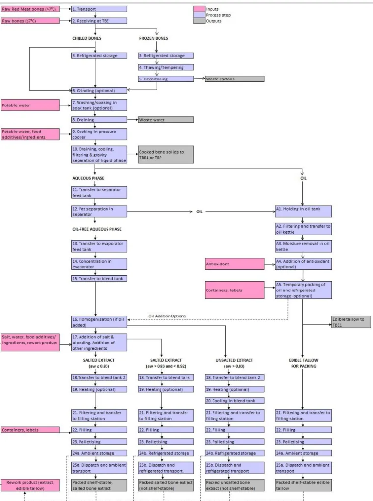
The extraction process takes place in Okaiawa (New Zealand North island, Taranaki region) on the plant of TBE III. Two kinds of products are manufactured there : beef leg bones extract (BLB) and beef mixed bones extract (BMB), which can both be used, among other things, for soups, sauces and fillings. For example, BLB is mostly produced for the Korean market as a basis for a traditional Korean soup.
The carcasses processed by TBE all come from animals bred and slaughtered in New Zealand. When TBE receive their raw material, mixed bones and leg bones are already separated. Mixed bones come into the plant at approximately 10°C and are usually treated quickly upon arrival (approximately 24h), whereas leg bones are supplied frozen and kept that way until enough material is gathered for a batch. Before being processed, bones go through back pressure rollers to be roughly crushed. They are then soaked for approximately 2h in water in order to remove as much blood as possible, as blood is believed to be responsible for extract coloration, which is not always desirable especially for BLB. However, as it is now, the cleaning step is not as efficient as expected.
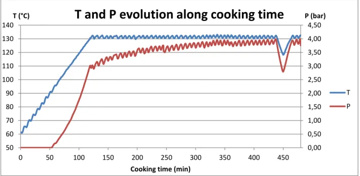
Once bones have been crushed and cleaned, they are loaded into the cooking baskets. Two cookers sit in TBE III, and each of them is large enough to contain two baskets (basket #2 sitting on top of basket #1). The cookers have a volume of 10 m3, with a diameter of about 2m. For a BLB batch, each basket is loaded with approximately 1.75 t of raw bones (3.5 t/cooker). Beef mixed bones being less dense than leg bones, only 1.5 t of raw material is loaded in each basket for a BMB batch (3 t/cooker). After loading the crushed bones in the basket, water is introduced into the pressure cooking vessels at 80°C for sanitary reasons, using a water to bone ratio of 2:1 w/w. The system temperature usually drops to around 50°C before it goes back up to the set extraction temperature thanks to a heat exchange where the heating fluid is superheated steam flowing around the cooker. No steam hits the product at any stage during the process, though, except of course for the steam resulting from water evaporation inside the cooker (liquid/vapor equilibrium). It takes about 2h for the set temperature to be reached, after what it is maintained at 131°C ± 2°C for an additional 2h for BMB and at 127°C ± 2°C for an additional 6h for BLB.
The inside temperature of the cooker (measured at its bottom) is controlled as follows : once the set temperature is reached, the heating steam flow stops until the temperature drops more than 2°C apart from it (i.e. below 125°C for BLB and 129°C for BMB). Only at this point will steam start flowing around the cooker again until the temperature is brought up to its set value. Moreover, each time steam circulation is on, a recirculating pump starts in order to homogenize the system. This pump brings the stock from the bottom of the cooking vessel to its top, and it also starts intermittently throughout the process, independently of temperature. The pressure inside the cooker (measured at its top) is around 2.5-3 bars (differential pressure) but it slightly rises each time stock is reheated until a maximum of 4 bars is reached and pressure is partly released. Working temperatures were determined empirically and the reason why
15 BLB is produced at a lower temperature is because higher working temperatures result in a darker colour of the extract, which is unwanted for this product.
The extraction procedure produces two phases : an aqueous phase (stock) with a viscosity of 5-8 Brix that is protein rich, and an oil phase (melted fat) which sits on top of the aqueous phase. After extraction, the liquid is removed from the bottom of the cooking vessels and transferred to a holding tank. During this process the liquor passes through two heat exchangers and its temperature drops from 130°C to 85°C. Moreover, during transfer, the liquid passes through an Ecofilter to remove all particulate matter (dark, overcooked small pieces of meat, present in larger quantities for BMB than for BLB). Due to their small size, these particles go through the basket perforations and can be found in the stock later on, hence the need of the filtration step.
The conductivity of the liquid is monitored continuously to check for the oil phase. Once oil is detected, the remaining liquid is diverted to an oil holding tank, which provides a preliminary oil separation. The stock then passes through two disc centrifuges for remaining oil to be removed before being collected in two holding tanks. As for the oil, it is filtered and concentrated under vacuum (82°C) to remove moisture (from 2 % to about 0.1 % moisture). Oil will be used later on, either to be added back in the product at the end of the process or to be sold separately. At this stage, the stock has a consistency of 5-8 Brix (5-10 % protein) and it goes through a double effect evaporator (vacuum, 75°C) to be concentrated to 55 Brix (45-50 % protein). This is the highest achievable concentration, as above 55 Brix the liquor becomes too viscous and blocks the evaporator plates. In some cases, especially for BLB (which has to be lighter in colour), oil is reintroduced and mixed with the stock using a homogenizer under 65-70°C.
The stock is either packed as a frozen perishable product, or crystallized sea salt is added (12 % of the final product) to reduce water activity and make it shelf stable. In this case, it is packed as a salt-added product. However, before being packed, the product is pasteurized as follows :
Salt added products are exposed to heat (80°C) for 10 min, before being cooled down to 60-65°C and hot filled in 20 kg bag-in-box.
Perishable products are exposed to heat (80°C) for 10 min, before being cooled down to 20-22°C in the storage tank, cool packed in plastic pails and chilled below 4°C.
The total time necessary to run a full batch, from loading the crushed bones into the cooking basket to packaging the final product, is 18h. At the end of a batch, the leftover bones (which look solid but can actually be easily crushed by hand) are sent to the rendering plant. This procedure of protein extraction provides 10x value addition to the raw material, and one run in the plant is roughly costed at 7000 NZD (about 5000 USD) A diagram summarizing the whole process is displayed on next page :
16 Fig. 1 : Beef bone protein extraction process flow diagram
17
II ; 3/ Involved phenomena
TBE’s process consists in performing a high temperature hydrolysis on beef bones. The working temperatures lie in the 125°C – 135°C range and therefore, the cooking step takes place under pressure. Bone hydrolysis at an industrial scale is usually performed in order to produce gelatin (collagen gel) but in this case, the working temperature would be much lower (in the 60°C -80°C range), as a high temperature is a hindrance to gel stability and strength. Moreover, for gelatin production, raw material is usually pre-treated (acid, alkali or enzymatic pre-treatment) and cooking often takes place in acidic conditions, as a simple hydrolysis with a non-pretreated raw material in this temperature range yields very poor results. TBE, on the other hand does not aim to produce gelatin but beef bone stock, which is liquid and protein-rich. Very little information could be found in the literature regarding the behavior of bone material and proteins at such a high temperature (130°C). Among all the publications I found, only one article, published by Dong et al in 2014 was reporting results obtained in conditions similar to those of TBE. In this article, called Development of a novel method for hot-pressure extraction of protein from chicken bone and the effect of enzymatic hydrolysis on the extract, the researchers report to have cooked chicken bones in water at 130°C for 2h and according to them, 80 % of initial bone proteins were recovered thanks to this method. This is a much better yield than what had been observed before, as previous studies reported that depending on the method of extraction, only 6.7-17.6% of total proteins from chicken bones could be recovered.[12]
Given the knowledge we had of TBE’s process and the information we gathered in the literature, we knew that the following phenomena were to be expected during high-temperature beef bone hydrolysis :
Heat transfer : For bones and bone proteins to undergo heat-induced modifications, they obviously need to be exposed to high temperatures. At the industrial scale, raw material is cooked in a large-dimension cooking basket of cylindrical shape. Each basket is about 1.4m large in diameter and therefore, we can reasonably expect heat transfer to display inertia, i.e. that time will be necessary for the central part of the cooker to be exposed to heat mainly coming from its sides. Heat transfer will occur via conduction through fluid and cooked material and via convection, as bones are immerged in circulating fluid. Moreover, depending on how densely it is packed inside the cooker, water and/or steam (resulting from the high temperature) will also circulate through the porous media (resulting from crushed bone pieces and scraps), thus increasing heat transfer.
Heat induced aggregation/gelation : According to Zhang et al (2009), “the thermal gelation process of globular proteins generally consists of three steps : thermal denaturation of proteins, followed by soluble aggregate formation from denatured or unfolded proteins, further association of the aggregates to form gel networks (if the protein concentration exceeds a given critical threshold concentration, and the environmental conditions other than protein concentration are specific). This process is affected by a considerable number of parameters, including pH, ionic strength, protein concentration, and heating conditions.”[13] This summary applies to globular proteins (such as hemoglobin or immunoglobins, for example), but we believe it also describes collagen behavior well enough. After proteins have been extracted from the raw material, their unfolding (due to heat exposure) exposes their hydrophobic parts, resulting in aggregation. We also have reasons to believe that when
18 exposed to high temperatures for a long time, proteins will tend to precipitate. Little information is available in the literature regarding the exact mechanisms of protein denaturation in our temperature and pH ranges, studies usually focusing on lower temperatures and non-neutral pH, whereas we worked under neutral/slightly acidic conditions and with high temperatures. Only very little gel formation was noticed at high temperatures. Proteins modifications : Due to a long exposure to water and heat, a number of structural
modifications are prone to appear on the extracted proteins, such as oxidation or deamidation, for example. Among those possible modifications, the occurring of Maillard reaction is of particular interest to us, given the fact that stock browning is noticed during the cooking step, and that it seems to be a critical parameter. Maillard reaction is a form of non-enzymatic browning, involving amino acids and reducing sugars. It is responsible for many colors and flavors in food, such as the browning of various meats when grilled, the darkened crust of bread, or malted barley (found in malt whisky or beer). The first step of Maillard reaction is a reaction between the sugar’s carbonyl group and the amino group of the amino acid, producing a Schiff base, a N-substituted glycosylamine and water. Depending on the nature of the reducing sugar, the N-glycosylamine will be rearranged, resulting in the formation of an Amadori intermediate or of a Heyns intermediate. After then, depending on pH, temperature and water activity, the reaction can go on in a large number of different manners, always resulting in the end in browning and in the formation of flavor compounds.
Proteins migration : Once proteins have been extracted from the initial solid material and are either dissolved or suspended in water, they start migrating for a homogeneous protein concentration to be reached in the system, according to Fick’s first law (Adolf Fick, 1855) : 𝐽 = −𝐷.𝜕𝐶
𝜕𝑥 where J is the diffusion flux (kg.m
-2
.s-1), D is the diffusivity (m².s-1), C is the concentration (kg.m-3) and x is the position (m). This equation tells us that, if a concentration gradient exists with regards to a particular species in a solution, then the considered species will migrate from high-concentration areas, to low-concentration areas, until equilibrium is reached. This obviously causes concentration to change along time, which is described by Fick’s second law : 𝜕𝐶𝜕𝑡 = 𝐷.𝜕2𝐶
𝜕𝑥2. In our case, proteins migration will be both diffusive (Fick’s law), but also forced, due to fluid (liquid water and steam) circulation inside the cooker.
19
III/ Material and methods
III ; 1/ Experimental design
III ; 1 ; 1/ Preliminary reflection
At the beginning of my internship in February 2015, before I came to work in Lincoln, AgResearch performed a number of runs in their cooker and sent INRA a first batch of results for us to analyze. The raw material that AgResearch used for their runs was mixed bones (46 % bone material, 54 % scraps), that were cooked at 122°C, 127°C and 132°C for eight hours in their lab scale pressure cooker, with three replicates for each temperature. For each of these runs, AgResearch took a 2 mL sample after 2h, 4h, 6h and 8h of cooking and performed mass spectrometry analysis on it. Mass spectrometry analysis provides data regarding the kind of damage inflicted to the proteins (oxidation, Maillard reaction, deamidation…), along with semi-quantitative data regarding the protein composition of the sample. However, even though we were able to determine which proteins were majority in the system (collagen, fibronectin, serum albumine, hemoglobin, myoglobin, myosin, actin, elastin, DNA, RNA, histone) the data regarding protein damage seemed to be a blur, as no clear tendency could be observed, whether we were looking at the influence of temperature or of cooking time. Moreover, the data were strongly divergent from one replicate to the other, so there was nothing we could be really sure of and there was no way we could start building a model from these results at INRA.
At this point, the main information we had about the process was that proteins were extracted from beef bones during a high temperature hydrolysis, usually around 130°C. We also knew that browning was observed during cooking, which we quickly related to the occurring of Maillard reaction, and that collagen was likely to be the main protein in the system. However, we immediately understood that the presence of bones, meat, fat and connective tissues all together in the raw material could be a hindrance to a clear interpretation of the data. In this regard, it was decided that during my stay in Lincoln, I would have to perform new runs in the pressure cooker after having separated bones from scraps in the raw material, even though this separation step does not exist in the process. The general idea was to try to understand the impact of each component of the system regarding :
Quantity of extracted proteins and extraction kinetics ; Occurring of non-enzymatic browning (Maillard reaction) ; Kind of extracted proteins ;
Undergone damage.
Regarding proteins extraction, we knew from past experience that when a process is complex, with various phenomena occurring simultaneously, apparent first order kinetics are to be expected in most cases. These are usually governed by an equation of the following kind :
𝑑𝐶(𝑡)
𝑑𝑡 = −𝑘. 𝐶(𝑡) where C(t) is the concentration of the observed reactant and k is a kinetic constant
However, in our case, we will focus on a product (extracted proteins) whose concentration will be rising along time, most likely tending towards a maximal value Cmax, Cmax being higher than C(t) at all times :
20 𝑑𝐶(𝑡) 𝑑𝑡 = 𝑘. (𝐶𝑚𝑎𝑥− 𝐶(𝑡)) ∫ 𝐶(𝑡)−𝐶1 𝑚𝑎𝑥 𝐶(𝑡) 𝐶0 . 𝑑𝐶(𝑡) = −𝑘. ∫ 𝑑𝑡 𝑡 0 𝑙𝑛 [𝐶(𝑡)−𝐶𝑚𝑎𝑥 𝐶0−𝐶𝑚𝑎𝑥 ] = −𝑘. 𝑡 𝐶(𝑡) = 𝐶𝑚𝑎𝑥− (𝐶𝑚𝑎𝑥− 𝐶0). 𝑒−𝑘.𝑡
If C0 = 0 g/L, then we have 𝐶(𝑡) = 𝐶𝑚𝑎𝑥. (1 − 𝑒−𝑘.𝑡) and the higher k is, the faster Cmax will be reached. Since we didn’t have any information regarding the extraction kinetics, we thought it would be pertinent to start sampling before 2h of cooking, as there was a possibility that not much was left to observe after then. The kind of equation described earlier indeed results in curves of the following type :
Fig. 2 : First order kinetics curve (focusing on product) (Courbe typique de la cinétique de premier ordre)
It also seemed to us that the working temperatures chosen by AgResearch were too close from one another for us to be able to see obvious differences. Thus, instead of working with only 5°C intervals, we decided to keep three working temperatures, but to choose them 20°C apart from one another. The working temperatures we selected were 130°C, 110°C and 90°C.
III ; 1 ; 2/ Building the definitive experimental design
The original experimental design as we had planned it for my two months in Lincoln was as follows : Cooking meat and bones in test tubes in a 90°C water bath in order to exhibit the main
tendencies regarding colour evolution and protein extraction ;
Conducting preliminary runs in the pressure cooker at 130°C while analyzing colour evolution and protein extraction kinetics to select the optimal set of sampling points ;
X(t) Time
C(t) = Cmax.(1-exp(-k.t))
k3 = 4*k1 k2 = 2*k1 k121 Cooking scraped mixed bones and meat scraps in the pressure cooker at 130°C, 110°C and 90°C with at least two replicates for each temperature, and measuring colour and protein concentration for each sample. The results obtained from these final runs would help us build a model at INRA during my last two months in Clermont-Ferrand. The obtained samples would be kept at AgResearch for further analysis to be conducted after my departure.
The first two runs that I conducted respectively consisted in meat (rump steak) and mixed bones (100 % bone material) cooked in test tubes (4g of raw material and 8g of water) plunged in an 85°C water bath (technical restrictions made it impossible to reach 90°C in a water bath). For each measurement point, three test tubes were taken out of the water bath and plunged in ice in order to stop any ongoing reactions. The purpose of these experiments was to be able to witness the colour evolution of the stock at all time (which would be impossible in the cooker) and to highlight a tendency in the extraction kinetics, while getting used to the concentration measurement method, which needs training to master. The obtained results showed that there was almost no extraction occurring when cooking meat at this temperature, but that 85°C was enough to extract proteins from bones. However, the extraction was slow and even if we suspect that a maximal concentration was reached at some point between 6h end 23h, we could not be absolutely sure of it, since we lacked measurement points between these two times as it can be seen on the chart below :
Fig. 3 : Meat and mixed bones cooking in an 85°C water bath : protein concentration (Cuisson de viande maigre et d’os mélangés dans un bain-marie à 85°C : concentration en protéines)
Regarding colour evolution, no browning was observed at this temperature for either kind of raw material. At this point, we concluded that the amount of extractible proteins was higher in bone material than in meat, but the cause of Maillard reaction was still unknown to us, even though our first assumption was that
0 2 4 6 8 10 12 14 16 0 200 400 600 800 1000 1200 1400 1600 Protein concentration (g/L)
Cooking time (min)
Meat and mixed bones cooking in an 85°C water
bath
Meat Mixed bones
22 meat was responsible for it. Indeed, sugars are necessary for Maillard reaction to occur and, bones containing very little of it (mainly in glycoproteins and proteoglycans, whose proportions are very low), we did not think bone sugar by itself could be the main cause of Maillard reaction.
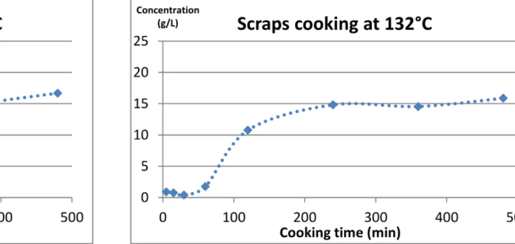
Following theses preliminary experiments, three runs were performed at 130°C in the pressure cooker (respectively beef rump steak, scraps, and scraped mixed bones). The chosen sampling times were 5 min, 15 min, 30 min, 1h, 2h, 4h, 6h and 8h. However, at this point a mixing defect in the pressure cooker was noticed (see Part IV ; 1) and it took us one week to fix it. Consequently, I was running out of time and I was not able to carry out all the runs that we had originally planned, especially given the fact that the results that I got from the first three runs in the cooker were mostly useless due to the bad mixing.
Therefore, I was able to collect results from runs performed on scraped mixed bones and scraps at 130°C, 110°C and 90°C, as planned, but I did not have enough time for any more replicates. Indeed, as each run takes a full working day worth of time to perform, and cleaning the cooker to have it ready for the next run is also time consuming, we lost approximately two weeks at this point, which would normally have been enough time to repeat every run. I did have enough time to perform one last run, though, using scraped leg bones at 130°C to check the behavior difference between the two types of bone material. For these final seven runs, the chosen sampling times were 5 min, 30 min, 1h, 1h30, 2h, 2h30, 3h, 4h, 5h, 6h, 8h and 10h.
III ; 2/ Analysis methods
The analysis methods we used to collect our results will be described in this part of the report. During my stay in Lincoln, I personally performed analysis regarding colour and protein concentration measurement. Mass spectrometry and amino acid analysis were performed by AgResearch’s researchers after my departure.
Colour measurement
Colour measurement was performed thanks to a UV spectrophotometer (Thermo Scientific Evolution 220). For each measurement, 1 mL of solution was collected with an Eppendorf 0.5 mL pipette and put in a cuvette. The solution was scanned with the following parameters being applied :
Wavelength range : 250 nm – 700 nm Integration time : 0.2 s
Wavelength step : 2 nm Scanning speed : 600 nm/min Bandwidth : 2 nm
Once the scan was over, a transmittance spectrum was obtained. The spectrum was imported in VisionLite ColorCalc (colour measurement software) for CIELAB (D65/2) values to be calculated. CIELAB is a color space specified by the International Commission on Illumination (in French, Commission Internationale de l'Eclairage, hence its CIE initialism). It describes all the colors visible to the human eye and was created to serve as a device-independent model to be used as a reference. The three coordinates of CIELAB represent the lightness of the color (L* = 0 yields black and L* = 100 indicates diffuse white), its position between red/magenta and green (a* varies between -128 and +127, negative values indicate green while positive
23 values indicate magenta) and its position between yellow and blue (b* varies between -128 and +127, negative values indicate blue and positive values indicate yellow). [14] Even though L* is commonly associated with lightness, we observed that in our case it was rather a measure of translucency, clear water scanning resulting in very high L* values (over 90) and opaque liquids scanning resulting in low L* values (even when they were light in colour).
The asterisks after L, a and b are part of the full name, since they represent L*, a* and b*, to distinguish them from Hunter's Lab (another colour standard based on the same principle as CIELAB but resulting in very different numerical values). Since the L*a*b* model is a three-dimensional model, it can be represented properly only in a three-dimensional space, as shown below :
Fig. 4 : CIE L*a*b* colour space (Représentation spatiale du modèle CIE L*a*b*)
Protein concentration measurement
Protein concentration was measured thanks to EMD Millipore’s Direct Detect spectrometer, whose technology is based on Infrared spectroscopy. IR spectroscopy exploits the fact that molecules absorb specific frequencies characteristic of their structure. To form a protein or a peptide, amino acids are covalently linked via amide (peptide) bonds. Amide bonds absorb electromagnetic radiation in multiple regions of the mid-IR spectrum, including the strong band at 1600-1690 cm-1. In order to determine protein and peptide concentration, the Direct Detect spectrometer measures the intensity (peak height) of the Amide I band, which is assigned to C=O stretching vibration of the peptide bond (about 80%) with a minor contribution from C-N stretching vibration (about 20%). According to the measured peak intensity, the number of peptide bonds is calculated and protein concentration is deduced.[15]
In order to perform the measurement, a drop (2 µL) of solution is to be put on a paper disk on a measuring card (4 disks/card, i.e. 4 possible measurements per card). Once the card has dried in free air during a few minutes, it is ready to be read by the machine. Direct Detect is only reliable when the measured concentration lies between 0.025 g/L and 5 g/L and therefore we worked with dilutions in most cases (5, 10 or 20x, LCMS-grade water being used as solvent). A picture of the spectrometer, along with the measurement cards, is displayed below :
24 Fig. 5 : Direct Detect spectrometer
(Spectromètre Direct Detect)
Amino acid analysis
Amino acid analysis consists in breaking proteins down to their free amino acids state and to determine the mass fraction of each amino acid in relation to the total solid material. Therefore, amino acid analysis allowed us to check both the protein concentration of the measured samples, along with their amino acid composition.
In order to be analyzed, each sample was dried, transferred to a glass hydrolysing tube and subjected to acid hydrolysis using HCl vapour at 110 °C for 24 h followed by phenylisothiocyanate derivatisation. Amino acid analysis was performed using an Ultimate 3000 HPLC system (Dionex). 10 µl of the derivatised samples was injected onto a Zorbax SB-C18, 5 μm, 250 x 4.6 mm column (Agilent Technologies) protected with a C18 guard column. The separation was performed at 40°C using a gradient from 2-40% mobile phase B over 31 min. Mobile phase A contained sodium acetate (140 mM), sodium azide (7.5 mM), disodium EDTA (0.26 mM) and triethylamine (20 mM) in water, and was titrated to pH 5.9 with acetic acid. Mobile phase B was 100% acetonitrile. The eluting peaks were monitored at 254 nm using a photodiode array detector (Ultimate 3000 PDA).
The level of tryptophan could not be determined by this method because the indole ring of this amino acid is highly sensitive to the acidic conditions. Three injection repeats for each sample were carried out for this analysis.
Mass spectrometry
Mass spectrometry (MS) is an analytical chemistry technique that helps identify the amount and type of chemicals present in a sample. In a typical MS procedure, a sample, which may be solid, liquid, or gas, is ionized, for example by bombarding it with electrons. This may cause some of the sample's molecules to break into charged fragments. These ions are then separated according to their mass-to-charge ratio, typically by accelerating them and subjecting them to an electric or magnetic field : ions of the same mass-to-charge ratio will undergo the same amount of deflection. The ions are detected by a mechanism capable of detecting charged particles, such as an electron multiplier. Results are displayed as spectra of the relative abundance of detected ions as a function of the mass-to-charge ratio. The atoms or molecules in
25 the sample can be identified by correlating known masses to the identified masses or through a characteristic fragmentation pattern.[16]
In our case, preliminary trypsin digestion was necessary for samples to be analyzed. Trypsin mostly cuts proteins at lysine and arginine, resulting in 5-30 AA long peptides. Each peptide which is taken into consideration by the measure is then related to its “mother protein” and modification scores can also be calculated. In our case, we looked for amino-acid modifications regarding oxidation, nitration, kynurenine/hydroxykynurenine, deamidation, dehydroalanine, dehydration and Maillard products. Each modification can only affect certain amino acids and each score is actually a percentage representing the number of amino acids bearing a modification in relation to the number of amino acids which could have born it. For example, only asparagine and glutamine are concerned by deamidation and therefore, deamidation score is calculated by dividing the number of deamidated Asn and Gln by the total number of Asn and Gln.
Each sample was prepared as follows :
In order to precipitate the proteins, 100 µL of liquid sample was mixed with 400 µL of methanol, 100 µL of chloroform and 300µL of water. The mix was then centrifuged for 1 min at 14000 rpm, resulting in the formation of 2 phases : an aqueous layer on top and an organic layer at the bottom, proteins sitting between the two phases. After the aqueous layer was removed, 400 µL of methanol was once again added, the mix was centrifuged at 14000 rpm for 2 min, methanol was removed and the sample was dried under a fume hood.
Proteins were resuspended via the addition of 100 µL of 50 mM Ammonium bicarbonate and 20 µL of 50 mM TCEP (tris(2-carboxyethyl)phosphine). The mix was incubated for 1h at room temperature and alkylated with 20 µL of 150 mM iodoacetamide. Trypsin digestion was then performed thanks to the addition of 10 µL of trypsin aliquots and 14 µL of CAN, before the sample was incubated at 37°C for 18h and dried.
The dried protein digests were resuspended in 100 µl of 0.1% formic acid and diluted 3 times prior to LC-MS/MS.
LC-MS/MS was performed on a nanoAdvance UPLC coupled to an amaZon speed ETD mass spectrometer equipped with a CaptiveSpray source (Bruker Daltonik). 5 μL of sample was loaded on a C18AQ nano trap (Bruker, 75 μm x 2 cm, C18AQ, 3 μm particles, 200 Å pore size). The trap column was then switched in line with the analytical column (Bruker Magic C18AQ, 100 μm x 15 cm C18AQ, 3 μm particles, 200 Å pore size). The column oven temperature was 50 °C. Elution was with a gradient from 0-25% B in 65 min, to 35% B in 75 min, total 90 min at a flow rate of 800 nl/min. Solvent A was LCMS-grade water with 0.1% FA and 1% ACN; solvent B was LCMS-grade ACN with 0.1% FA and 1% water. Samples were measured in auto MS/MS mode, with a mass range of m/z 350-1200. One MS was followed by 10 MS/MS of the most intense ions.
Raw LC-MS/MS data files were processed using Bruker DataAnalysis 4.2 to produce peaklists. These peaklists, after import into ProteinScape 3.1 (Bruker), were analysed using iterative proteomic search strategies, involving protein identification and modification searching with the Mascot search engine (Matrix Science). All searches used semitrypsin as the enzyme, allowing up to 1 missed cleavage (i.e. accepting peptides that have up to one internal lysine or arginine, which would normally be broken under 100% digestion efficiency), with a monoisotopic peptide tolerance of 0.1 Da and an MS/MS tolerance of 0.3 Da. Instrument specificity was electrospray ion trap. The database was Uniprot, taxonomy Bos taurus.
26 Following iterative searching, proteins and peptides were compiled into master lists for each replicate, and exported to Excel. An in-house developed collection of Visual Basic scripts was then used to further analyse the occurrence and frequency of the different modifications in relation to the total observed occurrence of each amino acid. The scores thus calculated allow simple comparison of samples.
III ; 3/ Experimental raw material preparation
Beef mixed bones and leg bones were bought at Lincoln supermarket and frozen at -25°C. While frozen, they were roughly cut in cubes of about 3x3x3 cm3 and put back in the freezer until further use. They were then unfrozen and kept in an ice box at low temperature while bone material and beef scraps were separated, using a kitchen knife and a scalpel. Scraped bones were packed in plastic bags (about 500 g/bag) and scraps in others (500 g/bag as well). In the case of leg bones, yellow marrow was also removed and put aside. This scraping step helped me to have a better understanding of the kind of raw material that was used for the process. The data I obtained is displayed in the table below, and I used some of it to build the tables that were given in part II ; 1 (tables 1 and 2 giving, the raw material composition).
Table 4 : Experimental raw material composition (Composition de la matière première utilisée en laboratoire)
Scraps were cut into thin slices with a kitchen knife and clean bones were crushed using AgResearch workshop’s equipment, as shown below :
Bone material type Mixed bones Leg bones Total treated mass (g) 7206 3132
Bone material mass (g) 3298 2257
Scraps mass (g) 3908 378
Yellow marrow mass (g) 0 497
Bone material % 45,8% 72,1%
Scraps % 54,2% 12,1%
27 Fig. 6 : AgResearch’s bone crushing equipment
(Matériel utilisé par AgResearch pour le broyage des os)
A small quantity of bones is to be loaded at the bottom of the cylinder. The piston is then put down above the bones and a manual hydraulic press is used to crush them. When the pressure under the piston reaches 2000 psi (137.9 bar), the piston is released, removed and crushed bones thus obtained are placed in a clean plastic bag. This method offers a very fine crushing of mixed bones, very different from what is obtained at TBE, where raw material goes through back pressure rollers (rough crushing). The large amount of blood released by mixed bones crushing allowed the cylinder to be lubricated, which made bones easy to remove from it. However, when dealing with leg bones the situation was different : leg bones being harder, denser and dryer, crushing them with this method resulted in a very tight-packed bone aggregate at the bottom of the cylinder, which was almost impossible to remove unless it was soaked in hot water for a while to be softened. Consequently, leg bones were not crushed but the pieces I obtained after scraping were small enough to fit in AgResearch’s cooker’s basket. However, it is likely that the non-crushing of leg bones influenced the results I got for this kind of material regarding protein diffusion in water, as we will later see. Raw material was then frozen at -25°C until being cooked.
III ; 4/ Design and working of the lab scale pressure cooker
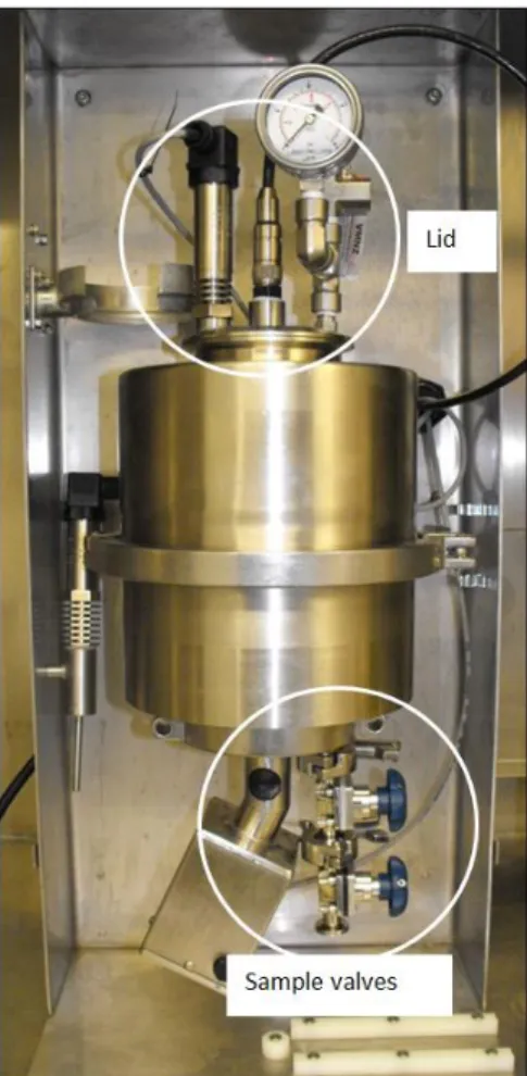
AgResearch’s pressure cooker was designed and built by the engineers of AgResearch’s workshop in Lincoln and can be seen below :
28 Fig. 7 : Assembled cooker, front view
(Cuiseur assemblé, vue de face)
The cooker is a small stainless steel tank with a volume of about 2L, surrounded by an electrical heating element and thermically insulated to minimize heat losses. The bottom part and the lid are fixed to the central tank using clamps (x2) and long screws. At the bottom, we can find the motor along with two removable sample valves. The motor can spin at a maximum speed of 800 rpm, but it is usually used at 400 or 600 rpm instead. An axis that cannot be seen on the picture connects it to a three-blade propeller at the bottom of the tank which is used to mix the liquid. On the lid, we can find the temperature probe in the center, along with a barometer and a pressure-reading gauge on the right. A security valve was also implemented, allowing steam to be released when the pressure inside the cooker exceeds 4 bars (differential pressure).
The motor, the temperature probe, the barometer and the heating element are all connected to a software interface, which allows the user to read the values of measured variables in real time, but also to set the following parameters before starting a run :
Working temperature : the temperature at which the heating should stop and that should be maintained afterwards ;
Heating time : the time that the heating element should take to bring the inside temperature from the initial temperature to the working temperature ;