HAL Id: hal-00654251
https://hal-enpc.archives-ouvertes.fr/hal-00654251
Submitted on 21 Dec 2011
HAL is a multi-disciplinary open access
archive for the deposit and dissemination of
sci-entific research documents, whether they are
pub-lished or not. The documents may come from
teaching and research institutions in France or
abroad, or from public or private research centers.
L’archive ouverte pluridisciplinaire HAL, est
destinée au dépôt et à la diffusion de documents
scientifiques de niveau recherche, publiés ou non,
émanant des établissements d’enseignement et de
recherche français ou étrangers, des laboratoires
publics ou privés.
Optimal aggregation of affine estimators
Joseph Salmon, Arnak S. Dalalyan
To cite this version:
Joseph Salmon, Arnak S. Dalalyan. Optimal aggregation of affine estimators. COLT - 24th Conference
on Learning Theory - 2011, Jul 2011, Budapest, Hungary. 19 p. �hal-00654251�
Optimal aggregation of affine estimators
Joseph Salmon
LPMA
Université Paris Diderot Paris 7 [email protected]
Arnak Dalalyan
LIGM / IMAGINE Université Paris Est / ENPC
Abstract
We consider the problem of combining a (possibly uncountably infinite) set of affine estima-tors in non-parametric regression model with heteroscedastic Gaussian noise. Focusing on the exponentially weighted aggregate, we prove a PAC-Bayesian type inequality that leads to sharp oracle inequalities in discrete but also in continuous settings. The framework is general enough to cover the combinations of various procedures—such as the least square regression, the kernel ridge regression, the shrinkage estimators, etc.—used in the literature on statisti-cal inverse problems. As a consequence, we show that the proposed aggregate provides an adaptive estimator in the exact minimax sense without neither discretizing the range of tun-ing parameters nor splitttun-ing the set of observations. We also illustrate numerically the good performance achieved by the exponentially weighted aggregate.
1 Introduction
There is a growing empirical evidence of superiority of aggregated statistical procedures, also referred to as blending, stacked generalization, or ensemble methods, with respect to “pure” ones. Since their introduction in the 1990’s, the most famous aggregation procedures such as Boosting (Freund, 1990),
Bagging (Breiman, 1996) or Random Forest (Amit and Geman, 1997) were successfully used in practice
for a large variety of applications. Moreover, the most recent Machine Learning competitions such as the Pascal VOC or the Netflix challenge were won by procedures combining different types of classifiers / predictors / estimators. It is therefore of central interest to understand from a theoretical point of view what kind of aggregation strategies should be used for getting the best possible combination of the available statistical procedures.
1.1 Historical remarks and motivation
In the statistical literature, to the best of our knowledge, the lecture notes of Nemirovski (2000) was the first work concerned by the theoretical analysis of aggregation procedures. It was followed by a paper by Juditsky and Nemirovski (2000), as well as by a series of papers by Catoni (see Catoni (2004) for a com-prehensive account) and Yang (2000, 2003, 2004). For the regression model, a significant progress was achieved by Tsybakov (2003) with introducing the notion of optimal rates of aggregation and proposing aggregation-rate-optimal procedures for the tasks of linear, convex and model selection aggregation. This point was further developed by Lounici (2007), Rigollet and Tsybakov (2007), Lecué (2007), Bunea et al. (2007), especially in the context of high dimension with sparsity constraints.
From a practical point of view, an important limitation of the previously cited results on the aggre-gation is that they are valid under the assumption that the aggregated procedures are deterministic (or random, but independent of the data used for the aggregation). In the Gaussian sequence model, a breakthrough was reached by Leung and Barron (2006). Building on a very elegant but not very well known result of George (1986), they established sharp oracle inequalities for the exponentially weighted aggregate (EWA) under the condition that the aggregated estimators are obtained from the data vector by orthogonally projecting it on some linear subspaces. Dalalyan and Tsybakov (2007, 2008), established the validity of Leung and Barron’s result under more general (non Gaussian) noise distributions provided that the constituent estimators are independent of the data used for the aggregation. A natural question arises whether a similar result can be proved for a larger family of constituent estimators containing projection estimators and deterministic ones as specific examples. The main aim of the present paper is to answer this question by considering families of affine estimators.
Our interest in affine estimators is motivated by several reasons. First of all, affine estimators encom-pass many popular estimators such as the smoothing splines, the Pinsker estimator Pinsker (1980), Efro-movich and Pinsker (1996), the local polynomial estimators, the non-local means Buades et al. (2005), Salmon and Le Pennec (2009), etc. For instance, it is known that if the underlying (unobserved) signal belongs to a Sobolev ball, then the (linear) Pinsker estimator is asymptotically minimax up to the opti-mal constant, while the best projection estimator is only rate-minimax. A second motivation is that—as proved by Juditsky and Nemirovski (2009)—the set of signals that are well estimated by linear estimators is very rich. It contains, for instance, sampled smooth functions, sampled modulated smooth functions and sampled harmonic functions (cf. Juditsky and Nemirovski (2009) for precise definitions). It is worth noting that oracle inequalities for the penalized empirical risk minimizer were also established by Gol-ubev (2010), and for the model selection by Arlot and Bach (2009), Baraud et al. (2010).
In the present work, we establish sharp oracle inequalities in the statistical model of heteroscedastic regression, under various conditions on the constituent estimators assumed to be affine functions of the data. We assume that the design is deterministic and that the noise is Gaussian with a given covari-ance matrix. Our results provide theoretical guarantees of optimality, in terms of the expected loss, for the exponentially weighted aggregate. They have the advantage of covering in a unified fashion the par-ticular cases of deterministic estimators considered by Dalalyan and Tsybakov (2008) and of projection estimators treated by Leung and Barron (2006).
1.2 Notation
Throughout this work, we focus on the heteroscedastic regression model with Gaussian additive noise.
More precisely, we assume that we are given a vector Y = (y1, ··· , yn)>∈ Rn obeying the model:
yi= fi+ ξi, for i = 1,...,n, (1)
whereξ = (ξ1, . . . ,ξn)> is a centered Gaussian random vector, fi = f(xi) where f is an unknown
func-tionX → R and x1, . . . , xn∈ X are deterministic points. Here, no assumption is made on the set X .
Our objective is to recover the vector f = (f1, . . . , fn), often referred to as signal, based on the data
y1, . . . , yn. In our work, the noise covariance matrixΣ = E[ξξ>] is assumed to be diagonal (so it can
be writtenΣ = diag(σ21, ··· ,σ2n)), with a known upper bound on the spectral norm k|Σk|. In our case,
k|Σk| = maxi =1,···,nσ2i. We measure the performance of an estimator ˆf by its expected empirical quadratic
loss: r = E(kf − ˆf k2n) where kf − ˆf k2n=n1
Pn
i =1( fi− ˆfi)
2. We also denote by 〈·|·〉
nthe corresponding
em-pirical inner product.
In this paper, we only focus on affine estimators ˆfλ, i.e., estimators that can be written as affine
transforms of the data Y = (y1, . . . , yn)>∈ Rn. Using the convention that all vectors are one-column
matrices, affine estimators can be defined by
ˆ
fλ= AλY + bλ, (2)
where the n × n real matrix Aλand the vector bλ∈ Rn are deterministic. This means that the entries of
Aλand bλmay depend on the points x1, . . . , xn but not on the data vector Y . It is well-known that the
quadratic risk of the estimator (2) is given by
rλ= E¡kf − ˆfλk2n¢ = k(Aλ− In×n) f + bλk2n+
Tr(AλΣA>λ)
n (3)
and that ˆrλ, defined by
ˆ rλ=° °Y − ˆfλ ° ° 2 n+ 2 nTr(ΣAλ) − 1 n n X i =1 σ2 i (4)
is an unbiased estimator of rλ(direct application of Stein’s Lemma, cf. Appendix).
Let us describe now different families of linear and affine estimators successfully used in the statis-tical literature (cf., for instance, Arlot and Bach (2009)). Our results apply to all these families and lead to a procedure that behaves nearly as well as the best one of the family.
Ordinary least squares Let {Sλ:λ ∈ Λ} be a set of linear subspaces of Rn. A well known family of affine estimators, successfully used in the context of model selection by Barron et al. (1999), is the set
of orthogonal projections ontoSλ. In the case of a family of linear regression models with design
matrices Xλ, one has Aλ= Xλ(Xλ>Xλ)−1Xλ>.
Diagonal filters Another set of common estimators are the so called diagonal filters ˆf = AY , where A is a diagonal matrix A = diag(a1, . . . , an). Popular examples include:
• Ordered projections : ak = 1l(k≤λ) for some integerλ (where 1l(·) is the indicator function).
Those weights are also called truncated SVD or spectral cut-off. In this case the natural
para-metrization isΛ = {1,...,n}, indexing the number of elements conserved.
• Block projections: ak= 1l(k≤w1)+
Pm−1
j =1 λj1l(wj≤k≤wj +1), k = 1,...,n, where λj ∈ {0, 1}. Here the
natural parametrization isΛ = {0,1}m−1, indexing subsets of {1, m − 1}.
• Tikhonov-Philipps filter: ak=1+(k/w)1 α, where w,α > 0. The set Λ = (R∗+)2indexes continuously
the smoothing parameters. • Pinsker filter: ak=¡1 −k
α w
¢
+, where x+= max(x, 0) and w, α > 0. In this case also Λ = (R∗+)2. Kernel ridge regression Assume that we have a positive definite kernel k :X × X → R and we aim at
estimating the true function f in the associated reproducing kernel Hilbert space (Hk, k · kk). The
kernel ridge estimator is obtained by minimizing the criterion kY − f k2n+ λk f k2kw.r.t. f ∈ Hk(see
(Shawe-Taylor and Cristianini, 2000, page 118)).Denoting by K the n ×n kernel-matrix with element
Ki , j= k(xi, xj), the unique solution ˆf is a linear estimate of the data, ˆf = AλY , with Aλ= K (K +
nλIn×n)−1, where I
n×nis the identity matrix of size n × n.
Multiple Kernel learning As proposed in Arlot and Bach (2009), it is also possible to handle the case
of several kernels k1, . . . , kM, with associated positive definite matrices K1, . . . , KM. For a parameter λ = (λ1, . . . ,λM) ∈ Λ = RM+ one can define the estimators ˆfλ= AλY with
Aλ=³ M X m=1 λmKm ´³ XM m=1 λmKm+ nIn×n ´−1 . (5)
It is worth mentioning that the formulation in Eq.(5) can be linked to the group Lasso Yuan and Lin (2006) and to the multiple kernel Lanckriet et al. (2003/04) — see Bach (2008), Arlot and Bach (2009) for more details.
1.3 Organization of the paper
In Section 2, we introduce EWA and state a PAC-Bayes type bound assessing the optimality of EWA in combining affine estimators. As a consequence, we provide in Section 3 sharp oracle inequalities in various set-ups: ranging from finite to continuous families of constituent estimators and including the sparsity scenario. In Section 4, we apply our main results to prove that combining Pinsker’s type filters with EWA leads to an asymptotically sharp adaptive procedure over the Sobolev ellipsoids. Section 5 is devoted to a numerical comparison of EWA with other classical filters (soft thresholding, blockwise shrinking, etc.), and illustrates the potential benefits of the aggregation. Some concluding remarks are presented in Section 6, while technical proofs are postponed to the Appendix.
2 Aggregation of estimators: main result
In this section we describe the statistical framework for aggregating estimators and we also introduce the exponentially weighted aggregate. The task of aggregation consists in estimating f by a suitable
combination of the elements of a family of constituent estimatorsFΛ= ( ˆfλ)λ∈Λ∈ Rn. The target
ob-jective of the aggregation is to build an aggregate ˆfaggr, not necessarily in the familyFΛ, that mimics
the performance of the best constituent estimator. It is called oracle because of its dependence on the
unknown function f . We assume thatΛ is a measurable subset of RM, for some M ∈ N.
The theoretical tool commonly used for evaluating the quality of an aggregation procedure is the oracle inequality (OI), generally written in the following form:
Ek ˆfaggr− f k2n≤ Cninf λ∈Λ ³ Ek ˆfλ− f k2n ´ + Rn, (6)
with residual term Rn tending to zero, and leading constant Cn being bounded. The OIs with leading
constant one are of central theoretical interest since they allow to bound the excess risk and to assess
the aggregation-rate-optimality. The residual term Rn depends on the complexity (size) of the family
2.1 Exponentially Weighted Aggregate (EWA)
Let rλ= E(k ˆfλ− f k2n) denote the risk of the estimator ˆfλ, for anyλ ∈ Λ, and let ˆrλbe an estimator of rλ.
The precise form of ˆrλstrongly depends on the nature of the constituent estimators. For any probability
distributionπ over the set Λ and for any β > 0, we define the probability measure of exponential weights,
ˆ
π, by the following formula:
ˆ
π(dλ) = θ(λ)π(dλ) with θ(λ) =R exp(−n ˆrλ/β)
Λexp(−n ˆrω/β)π(dω). (7)
The corresponding exponentially weighted aggregate, henceforth denoted by ˆfEWA, is the expectation of
the ˆfλw.r.t. the probability measure ˆπ:
ˆ fEWA= Z Λ ˆ fλπ(dλ).ˆ (8)
It is convenient and customary to use the terminology of Bayesian statistics: the measureπ is called
prior, the measure ˆπ is called posterior and the aggregate ˆfEWAis then the posterior mean. The parame-terβ will be referred to as the temperature parameter. In the framework of aggregating statistical proce-dures, the use of such an aggregate can be traced back to George (1986).
The interpretation of the weights θ(λ) is simple: they up-weight estimators all the more that their
performance, measured in terms of the risk estimate ˆrλ, is good. The temperature parameter reflects the
confidence we have in this criterion: if the temperature is small (β ≈ 0) the distribution concentrates on
the estimators achieving the smallest value for ˆrλ, assigning almost zero weights to the other estimators.
On the other hand, ifβ → +∞ then the probability distribution over Λ is simply the prior π, and the
data do not modify our confidence in the estimators. It should also be noted that averaging w.r.t. the
posterior ˆπ is not the only way of constructing an estimator of f , some alternative estimators based on
ˆ
π have been studied, see for instance Zhang (2006), Audibert (2009).
2.2 Main result
To state our main result, we denote byPΛthe set of all probability measures onΛ and by K (p,p0) the
Kullback-Leibler divergence between two probability measures p, p0∈ P
Λ: K (p,p0) = (R Λlog ³d p d p0(λ) ´ p(dλ) if p ¿ p0, +∞ otherwise..
Theorem 1 (PAC Bayesian Bound) If either one of the following conditions is satisfied:
C1: The matrices Aλare orthogonal projections (i.e., symmetric and idempotent) and the vectors bλ
sat-isfy Aλbλ= 0, for all λ ∈ Λ.
C2: The matrices Aλare all symmetric, positive semidefinite and satisfy AλAλ0= Aλ0Aλ, AλΣ = ΣAλfor
allλ,λ0∈ Λ. All the vectors bλare zero.
Then, the risk of the aggregate ˆfEWAdefined by Equations (7), (8) and (4) satisfies the inequality
rEWA= E(k ˆfEWA− f k
2 n) ≤ inf p∈PΛ µZ ΛE ³° ° ˆfλ− f ° ° 2 n ´ p(dλ) +β nK (p,π) ¶ (9)
provided thatβ ≥ αk|Σk|, where α = 4 if C1holds true andα = 8 if C2holds true.
All the proofs of our results are given in the appendix, at the end of the paper.
Note also that the result of Theorem 1 applies to the estimator ˆfEWAthat uses the full knowledge of
the covariance matrixΣ. Indeed, even if for the choice of β only an upper bound on the spectral norm of
Σ is required, the entire matrix Σ enters in the definition of the unbiased risks ˆrλthat is used for defining
ˆ
fEWA. The exponentially weighted aggregate ˆfEWAis easily extended to handle the more realistic situation
where an unbiased estimateΣ, independent of Y , of the covariance matrix Σ is available. Simply replaceb
Σ bybΣ in the definition of the unbiased risk estimate (4). When the estimators ˆfλsatisfyπ-a.e. condition
C1or C2, choosingβ = αk| ˆΣk|, it can be checked that a claim similar to Theorem 1 remains valid.
Another observation is that using the extension of Stein’s lemma presented in (Dalalyan and Tsy-bakov, 2008, Lemma 1), a result similar to Theorem 1 can be established for some specific non Gaussian noise distributions, provided that the components of the noise vector are independent.
3 Sharp oracle inequalities
In this section, we discuss consequences of the main result for specific choices of prior measures. Some of them are closely related to the oracle inequalities presented in Dalalyan and Tsybakov (2007, 2008), Alquier and Lounici (2010), Rigollet and Tsybakov (2011) especially when dealing with the sparsity sce-nario in the high dimensional framework.
3.1 Discrete oracle inequality
In order to demonstrate that Inequality (9) can be reformulated in terms of an OI as defined by (6), let us
consider the simple case when the priorπ is discrete. That is, we assume that π(Λ0) = 1 for a countable
setΛ0⊂ Λ. Without loss of generality, we assume that Λ0= N. Then, the following result holds true.
Proposition 1 If either one of the conditions C1and C2(cf. Theorem 1) is fulfilled andπ is supported by
N, then the aggregate ˆfEWAdefined by Equations (7), (8) and (4) satisfies the inequality
E(k ˆfEWA− f k 2 n) ≤ inf j ∈N:πj>0 µ Ek ˆfj− f k2n+ βlog(1/πj) n ¶ (10)
provided thatβ ≥ αk|Σk|, where α = 4 if C1holds true andα = 8 if C2holds true.
Proof: It suffices to apply Theorem 1 and to bound the RHS from above by the minimum over all Dirac
measures p = δj with j such thatπj> 0.
3.2 Continuous oracle inequality
It may be useful in practice to combine a family of affine estimators indexed by an open subset ofRM,
for some integer M > 0, for instance when the aim is to build an estimator that is nearly as accurate as the best kernel estimator with fixed kernel and varying bandwidth. In order to state an oracle inequality
in such a “continuous” setup, let us denote by d2(λ,Λ) the largest real τ > 0 such that the ball centered
atλ with radius τ is included in Λ. In what follows, Leb(·) stands for the Lebesgue measure.
Proposition 2 LetΛ ⊂ RM be an open and bounded set and letπ be the uniform probability on Λ. As-sume that the mappingλ 7→ rλis Lipschitz continuous, i.e., |rλ0− rλ| ≤ Lrkλ0− λk2, ∀λ,λ0∈ Λ. Under the
conditions C1or C2aggregate ˆfEWAsatisfies the inequality Ek ˆfEWA− f k 2 n≤inf λ∈Λ n Ek ˆfλ− f k2n+ βM n log ³ p M 2 min(n−1, d 2(λ,Λ)) ´o +Lr+ β log¡Leb(Λ)¢ n . (11)
for everyβ ≥ αk|Σk| where α = 4 if C1holds true andα = 8 if C2holds true. 3.3 Sparsity oracle inequality
The continuous oracle inequality stated in previous subsection is well adapted to the case where the
dimension M ofΛ is small compared to the sample size n (or, more precisely, the signal to noise ratio
n/ maxiσ2i). If this is not the case, the choice of the prior should be done more carefully. For instance,
consider the case of a setΛ ⊂ RMwith large M under the sparsity scenario: there is a sparse vectorλ∗∈ Λ
such that the risk of ˆfλ∗ is small. Then, it is natural to choose a priorπ that promotes the sparsity of
λ. This can be done in the same vein as in Dalalyan and Tsybakov (2007, 2008), by means of the heavy
tailed prior: π(dλ) ∝YM j =1 1 (1 + |λj/τ|2)2 1lΛ(λ)d(λ), (12)
whereτ > 0 is a tuning parameter.
Proposition 3 LetΛ = RM and letπ be defined by (12). Assume that the mapping λ 7→ rλis continuously differentiable and, for some M × M matrix M , satisfies:
rλ− rλ0− ∇rλ>0(λ − λ0) ≤ (λ − λ0)>M (λ − λ0), ∀λ, λ0∈ Λ. (13)
If either one of the conditions C1and C2 (cf. Theorem 1) is fulfilled, then the aggregate ˆfEWAdefined by
Equations (7), (8) and (4) satisfies the inequality
E¡k ˆfEWA− f k 2 n¢ ≤ inf λ∈RM n Ek ˆfλ− f k2n+ 4β n M X j =1 log³1 +|λj| τ ´o + Tr(M )τ2 (14)
Let us discuss here some consequences of this sparsity oracle inequality. First of all, let us remark that
in most cases Tr(M ) is on the order of M and the choice τ = pβ/(nM) ensures that the last term in
the RHS of Eq. (14) decreases at the parametric rate 1/n. This is the choice we recommend for practical applications.
Assume now that we are given a large number of linear estimators ˆg1= G1Y , . . . , ˆgM= GMY
sat-isfying, for instance, condition C2. We will focus on matrices Gj having a spectral norm bounded by
one (it is well known that the failure of this condition makes the linear estimator inadmissible, cf. Co-hen (1966)). Assume furthermore that our aim is to propose an estimator that mimics the behavior of
the best possible convex combination of a pair of estimators chosen among ˆg1, . . . , ˆgM. This task can
be accomplished in the framework of the present paper by settingΛ = RM and ˆfλ= λ1gˆ1+ . . . λMgˆM,
whereλ = (λ1, . . . ,λM). If the collection { ˆgi} satisfies condition C2, then it is also the case for the
col-lection of their linear combinations { ˆfλ}. Moreover, the mappingλ 7→ rλ is quadratic with the
Hes-sian matrix ∇2rλ given by the entries 2〈Gjf |Gj0f 〉n+2nTr(Gj0ΣGj), j , j0= 1, . . . , M. This implies that
Inequality (13) holds withM being the Hessian divided by 2. Therefore, setting σ = (σ1, . . . ,σn), we get
Tr(M ) ≤ k|PMj =1G2jk|(k f k2n+ kσk2n) ≤ M(kf k2n+ kσk2n), where the norm of a matrix is understood as its
largest singular value. Applying Proposition 3 withτ = pβ/(nM), we get for β ≥ 8k|Σk|,
E¡k ˆfEWA− f k 2 n¢ ≤ inf α,j,j0Ekα ˆgj+ (1 − α) ˆgj0− f k 2 n+ 8β n log à 1 + s Mn β ! +β n(kf k 2 n+ kσk2n), (15)
where the inf is taken over allα ∈ [0,1] and j, j0∈ {1, . . . , M}. This shows that, using EWA with a
suf-ficiently large temperature, one can achieve the best possible risk over the convex combinations of a pair of linear estimators—selected from a large (but finite) family—at the price of a residual term that decreases at the parametric rate up to a log factor.
3.4 Oracle inequalities for varying-block-shrinkage estimators
Let us consider now the problem of aggregation of two-block shrinkage estimators. It means that the
constituent estimators have the following form: forλ = (a,b,k) ∈ [0,1]2× {1, . . . , n} := Λ, ˆfλ= AλY where
Aλ= diag¡a1l(i ≤ k) + b1l(i > k),i = 1,··· ,n¢. Let us choose the prior π as the uniform probability
distri-bution on the setΛ.
Proposition 4 Let ˆfEWA be the exponentially weighted aggregate having as constituent estimators
two-block shrinkage estimators AλY . IfΣ is a diagonal matrix, then for any λ ∈ Λ and for any β ≥ 8k|Σk|, E(k ˆfEWA− f k 2 n) ≤ E(k ˆfλ− f k2n) + β n n 1 + log³n 2k f k2 n+ n Tr(Σ) 12β ´o . (16)
The proof of this result can be found in Dalalyan and Salmon (2011).
In the caseΣ = In×n, this result is comparable to (Leung, 2004, page 20, Theorem 2.49), which states
that in the model of homoscedastic regression (Σ = In×n), the EWA acting on two-block positive-part
James-Stein shrinkage estimators satisfies, for any k = 3,··· ,n − 3, and for β = 8, the oracle inequality E(k ˆfLeung− f k2n) ≤ E(k ˆfλ− f k2n) +
9 n+ 8 nminK >0 n K ∨³logn − 6 K − 1 ´o . (17)
4 Application to minimax adaptive estimation
In the celebrated paper Pinsker (1980)proved that in the model (1) the minimax risk over ellipsoids
can be asymptotically attained by a linear estimator. Let us denote by θk( f ) = 〈f |ϕk〉n the
coeffi-cients of the (orthogonal) discrete sine transform of f , hereafter denoted byD f . Pinsker’s result—
restricted to Sobolev ellipsoidsF (α,R) = ©f ∈ Rn:Pn
k=1k
2αθ
k( f )2≤ Rª and to the homoscedastic noise
(Σ = σ2In×n)—states that, as n → ∞, the equivalences
inf ˆ f sup f ∈F (α,R) E¡k ˆf − f k2 n¢ ∼ inf A f ∈F (α,R)sup E¡kAY − f k 2 n ¢ (18) ∼ inf w >0f ∈F (α,R)sup E¡kAα,wY − f k 2 n ¢ (19)
hold (Tsybakov, 2009, Theorem 3.2), where the first inf is taken over all possible estimators ˆf and Aα,w=
D>diag¡(1 − kα/w )
+; k = 1,...,n
¢
D is the Pinsker filter in the discrete sine basis. In simple words, this implies that the (asymptotically) minimax estimator can be chosen from the quite narrow class of linear
estimators with Pinsker’s filter. However, it should be emphasized that the minimax linear estimator
depends on the parametersα and R, that are generally unknown. An (adaptive) estimator, that does
not depend on (α,R) and is asymptotically minimax over a large scale of Sobolev ellipsoids has been
proposed by Efromovich and Pinsker (1984). The next result, that is a direct consequence of Theorem 1, shows that EWA with linear constituent estimators is also asymptotically sharp adaptive over Sobolev ellipsoids.
Proposition 5 Letλ = (α,w) ∈ Λ = R2+and consider the prior π(dλ) = 2n−α/(2α+1)σ
¡1 + n−α/(2α+1)
σ w¢3
e−αdαdw, (20)
where nσ= n/σ2. Then, in model (1) with homoscedastic errors, the aggregate ˆf
EWAbased on the
tempera-tureβ = 8σ2and the constituent estimators ˆfα,w= Aα,wY (with Aα,wbeing the Pinsker filter) is adaptive in the exact minimax sense1on the family of classes {F (α,R) : α > 0,R > 0}.
It is worth noting that the exact minimax adaptivity property of our estimator ˆfEWAis achieved
with-out any tuning parameter. All previously proposed methods that are provably adaptive in exact minimax sense depend on some parameters such as the lengths of blocks for blockwise Stein and Efromovich-Pinsker estimators or the step of discretization and the maximal value of bandwidth Cavalier et al.
(2002). Another nice property of the estimator ˆfEWAis that it does not require any pilot estimator based
on the data splitting device Efromovich (1996), Yang (2004).
5 Experiments
In this section we present some numerical experiments on synthetic data, by focusing only on the case
of homoscedastic Gaussian noise (Σ = σ2In×n) with known variance. Following the philosophy of
repro-ducible research, a toolbox is made available freely for download at:
www.math.jussieu.fr/~salmon/code/index_codes.php
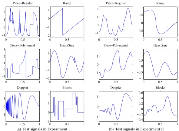
We evaluate different estimation routines on several 1D signals, introduced by Donoho and John-stone (1994, 1995) and considered as benchmark in literature on signal processing. The six signals we retained for our experiments because of their diversity are depicted in Figure 1. Since all these sig-nals are non-smooth, we have also carried out experiments on their smoothed versions obtained by taking an antiderivative, see Figure 1. In what follows, the experiment on non-smooth signals will be referred to as Experiment I, whereas the experiment on their smoothed counterparts will be referred to as Experiment II. In both cases, prior to applying estimation routines, we normalize the (true) sampled signal to have an empirical norm equal to one and use the Discrete Sine Transform (DST) denoted by θ(Y ) = ¡θ1(Y ), . . . ,θn(Y )
¢> .
The four estimation routines—including EWA—used in our experiments are detailed below:
Soft Thresholding (ST), Donoho and Johnstone (1994): For a given threshold parameter t , the soft
thresh-olding estimator of the vector of DST coefficientsθk( f ) is defined by
b θk= sgn ¡ θk(Y )¢¡|θk(Y )| − σt ¢ +. (21)
In our experiments, we use the threshold minimizing the estimated unbiased risk defined via Stein’s lemma. This procedure is referred to as SURE-shrink in Donoho and Johnstone (1995).
Blockwise James-Stein (BJS) shrinkage, Cai (1999): The set of indices {1, ··· ,n} is partitioned into N =
[n/ log(n)] non-overlapping blocks B1, B2, ···BN of equal size L. (If n is not a multiple of N , the
last block may be of smaller size than all the others.) The corresponding blocks of true coefficients
θBk( f ) =
¡
θj( f )¢j ∈B
k are estimated by shrinking the blocks of noisy coefficientsθBk(Y ):
b θBk= Ã 1 −λLσ 2 Sk2(Y )σ ! + θBk(Y ), k = 1,··· , N (22) where S2k(Y ) = kθBk(Y )k 2 2andλ = 4.50524 as in Cai (1999). 1see (Tsybakov, 2009, Definition 3.8)
0 0.5 1 −1 0 1 2 Piece−Regular 0 0.5 1 −2 −1 0 1 Ramp 0 0.5 1 −1 0 1 2 3 Piece−Polynomial 0 0.5 1 −2 −1 0 1 HeaviSine 0 0.5 1 −1 0 1 Doppler 0 0.5 1 −1 0 1 2 Blocks
(a) Test signals in Experiment I
0 0.5 1 −1 0 1 2 Piece−Regular 0 0.5 1 −0.5 0 0.5 1 Ramp 0 0.5 1 −1 0 1 Piece−Polynomial 0 0.5 1 −1 −0.5 0 0.5 1 HeaviSine 0 0.5 1 −1 0 1 Doppler 0 0.5 1 −0.4 −0.2 0 0.2 0.4 0.6 Blocks
(b) Test signals in Experiment II
Figure 1: Test signals used in our experiment: Piece-Regular, Ramp, Piece-Polynomial, HeaviSine, Doppler and Blocks. (a) non-smooth (Experiment I) and (b) smooth (Experiment II).
Unbiased risk estimate (URE) minimization, Golubev (1992), Cavalier et al. (2002): it consists in using
a Pinsker filter, as defined in Section 4, with a data-driven choice of parametersα and w. This
choice is done by minimizing an unbiased estimate of the risk over a suitably chosen grid for the
values ofα and w. Here, we use geometric grids ranging from 0.1 to 100 for α and from 1 to n for
w . The bi-dimensional grid used in all the experiments has 100×100 elements. We refer to Cavalier
et al. (2002) for the closed-form formula of the unbiased risk estimator.
EWA on Pinsker’s filters: We consider the same finite family of linear smoothers—defined by Pinsker’s
filters—as in the URE routine described above. According to Proposition 1, this leads to an estima-tor which is nearly as accurate as the best Pinsker’s estimaestima-tor in the given finite family.
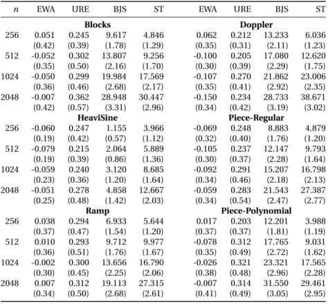
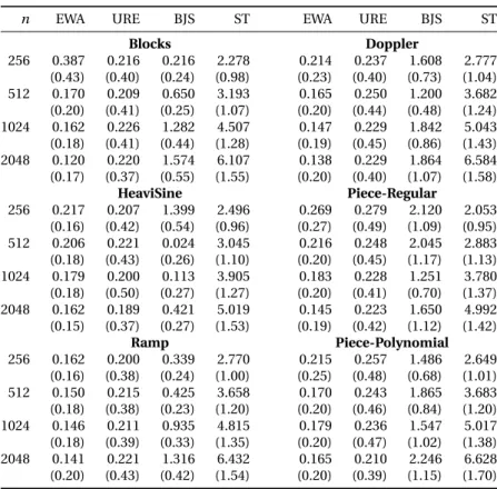
To report the result of our experiments, we have also computed the best linear smoother based on a Pinsker filter chosen among the candidates that we used for defining URE and EWA routines. By best smoother we mean the one minimizing the squared error, which can be computed since we know the ground truth. This pseudo-estimator will be referred to as oracle. The results summarized in Table 1 for Experiment I and Table 2 for Experiment II correspond to the average over 1000 trials of the mean squared error (MSE) from which we subtract the MSE of the oracle and multiply the resulting difference by the sample size. We report the results forσ = 0.33 and for n ∈ {28, 29, 210, 211}.
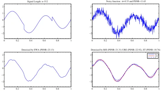
Simulations show that EWA and URE have very comparable performances and are significantly more accurate than Soft Thresholding and Block James-Stein (see Table 1) for every size n of signals consid-ered. The improvement is particularly important when the signal has large peaks (cf. Figure 2) or dis-continuities (cf. Figure 3). In most cases, the EWA method also outperforms URE, but this difference is much less pronounced. One can also observe that in the case of smooth signals, the difference of the MSEs between EWA and the oracle, multiplied by n, remains nearly constant when n varies. This is in perfect agreement with our theoretical results in which the residual term decreases to zero inversely proportionally to the sample size.
Of course, soft thresholding and blockwise James-Stein procedures have been designed for being applied to the wavelet transform of a Besov smooth function, rather than to the Fourier transform of a Sobolev-smooth function. However, the point here is not to demonstrate the superiority of EWA as com-pared to ST and BJS procedures. The point is to stress the importance of having sharp adaptivity up to
0 0.2 0.4 0.6 0.8 1 −2 −1 0 1 2 Signal Length: n=512 0 0.2 0.4 0.6 0.8 1 −2 −1 0 1 2
Noisy function : σ=0.33 and PSNR=11.63
0 0.2 0.4 0.6 0.8 1 −2 −1 0 1 2 Denoised by EWA (PSNR=23.13) 0 0.2 0.4 0.6 0.8 1 −2 −1 0 1 2 Denoised by BJS (PSNR=21.31) URE (PSNR=22.92), ST (PSNR=18.76) BJS URE ST
Figure 2: Heavisine. The first row is the true signal (left) and a noisy version corrupted by Gaussian noise
with standard deviationσ = 0.33 (right). The second row gives denoised version obtained by EWA (left),
BJS, ST and URE (right). The PSNR is computed by the formula PSNR = 10log10¡max(f )2/MSE¢.
0 0.2 0.4 0.6 0.8 1 −1 0 1 2 3 Signal Length: n=1024 0 0.2 0.4 0.6 0.8 1 −1 0 1 2 3
Noisy function : σ=0.33 and PSNR=17.44
0 0.2 0.4 0.6 0.8 1 −1 0 1 2 3 Denoised by EWA (PSNR=24.84) 0 0.2 0.4 0.6 0.8 1 −1 0 1 2 3 Denoised by BJS (PSNR=22.91) URE (PSNR=24.75), ST (PSNR=20.38) BJS URE ST
Figure 3: Piece-Regular. The first row is the true signal (left) and a noisy version corrupted by
Gaus-sian noise with standard deviation σ = 0.33 (right). The second row gives denoised version
ob-tained by EWA (left) and by BJS, ST and URE (right). The PSNR is computed by the formula PSNR = 10 log10¡max(f )2/MSE¢.
optimal constant and not simply adaptivity in the sense of rate of convergence. Indeed, the procedures ST and BJS are provably rate-adaptive when applied to Fourier transform of a Sobolev-smooth function, but they are not sharp adaptive—they do not attain the optimal constant—whereas EWA and URE do attain.
6 Summary and future work
In this paper, we have addressed the problem of aggregating a set of affine estimators in the context of regression with fixed design and heteroscedastic noise. Under some assumptions on the constituent
0 0.2 0.4 0.6 0.8 1 −2 0 2 4 Signal Length: n=1024 0 0.2 0.4 0.6 0.8 1 −2 0 2 4
Noisy function : σ=1 and PSNR=8
0 0.2 0.4 0.6 0.8 1 −2 0 2 4 Denoised by EWA (PSNR=19.64) 0 0.2 0.4 0.6 0.8 1 −2 0 2 4 Denoised by BJS (PSNR=16.8) URE (PSNR=19.59), ST (PSNR=15.16) BJS URE ST
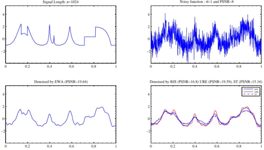
Figure 4: Piece-Regular. The first row is the true signal (left) and a noisy version corrupted by
Gaus-sian noise with standard deviation σ = 1 (right). The second row gives denoised version obtained
by EWA (left) and by BJS, ST and URE (right). The PSNR is computed by the formula PSNR =
10 log10¡max(f )2/MSE¢.
estimators, we have proven that the EWA with a suitably chosen temperature parameter satisfies PAC-Bayesian type inequality, from which different types of oracle inequalities have been deduced. All these inequalities are with leading constant one and with rate-optimal residual term. As a by-product of our results, we have shown that EWA applied to the family of Pinsker’s estimators produces an estimator, which is adaptive in the exact minimax sense. Next in our agenda is carrying out an experimental evalu-ation of the proposed aggregate using the approximevalu-ation schemes described by Dalalyan and Tsybakov (2009), Rigollet and Tsybakov (2011) and Alquier and Lounici (2010). It will also be interesting to extend the results of this work to the case of the unknown noise variance in the same vein as in Giraud (2008).
Acknowledgments
The authors acknowledge the support of the French Agence Nationale de la Recherche (ANR) under the grant PARCIMONIE.
References
P. Alquier and K. Lounici. Pac-bayesian bounds for sparse regression estimation with exponential
weights. Electron. J. Statist., 5:127–145, 2010.
Y. Amit and D. Geman. Shape quantization and recognition with randomized trees. Neural Comput., 9: 1545–1588, October 1997.
S. Arlot and F. Bach. Data-driven calibration of linear estimators with minimal penalties. In NIPS, pages 46–54, 2009.
J-Y. Audibert. Fast learning rates in statistical inference through aggregation. Ann. Statist., 37(4):1591– 1646, 2009.
F. Bach. Consistency of the group lasso and multiple kernel learning. J. Mach. Learn. Res., 9:1179–1225, 2008.
Y. Baraud, Ch. Giraud, and S. Huet. Estimator selection in the gaussian setting. submitted, 2010. A. R. Barron, L. Birgé, and P. Massart. Risk bounds for model selection via penalization. Probab. Theory
Related Fields, 113(3):301–413, 1999.
n EWA URE BJS ST EWA URE BJS ST Blocks Doppler 256 0.051 0.245 9.617 4.846 0.062 0.212 13.233 6.036 (0.42) (0.39) (1.78) (1.29) (0.35) (0.31) (2.11) (1.23) 512 -0.052 0.302 13.807 9.256 -0.100 0.205 17.080 12.620 (0.35) (0.50) (2.16) (1.70) (0.30) (0.39) (2.29) (1.75) 1024 -0.050 0.299 19.984 17.569 -0.107 0.270 21.862 23.006 (0.36) (0.46) (2.68) (2.17) (0.35) (0.41) (2.92) (2.35) 2048 -0.007 0.362 28.948 30.447 -0.150 0.234 28.733 38.671 (0.42) (0.57) (3.31) (2.96) (0.34) (0.42) (3.19) (3.02) HeaviSine Piece-Regular 256 -0.060 0.247 1.155 3.966 -0.069 0.248 8.883 4.879 (0.19) (0.42) (0.57) (1.12) (0.32) (0.40) (1.76) (1.20) 512 -0.079 0.215 2.064 5.889 -0.105 0.237 12.147 9.793 (0.19) (0.39) (0.86) (1.36) (0.30) (0.37) (2.28) (1.64) 1024 -0.059 0.240 3.120 8.685 -0.092 0.291 15.207 16.798 (0.23) (0.36) (1.20) (1.64) (0.34) (0.46) (2.18) (2.13) 2048 -0.051 0.278 4.858 12.667 -0.059 0.283 21.543 27.387 (0.25) (0.48) (1.42) (2.03) (0.34) (0.54) (2.47) (2.77) Ramp Piece-Polynomial 256 0.038 0.294 6.933 5.644 0.017 0.203 12.201 3.988 (0.37) (0.47) (1.54) (1.20) (0.37) (0.37) (1.81) (1.19) 512 0.010 0.293 9.712 9.977 -0.078 0.312 17.765 9.031 (0.36) (0.51) (1.76) (1.67) (0.35) (0.49) (2.72) (1.62) 1024 -0.002 0.300 13.656 16.790 -0.026 0.321 23.321 17.565 (0.30) (0.45) (2.25) (2.06) (0.38) (0.48) (2.96) (2.28) 2048 0.007 0.312 19.113 27.315 -0.007 0.314 31.550 29.461 (0.34) (0.50) (2.68) (2.61) (0.41) (0.49) (3.05) (2.95)
Table 1: Comparison of several adaptive methods on the six (non-smooth) signals of interest. For each
signal length n and each method, we give the average value of n×(MSE−MSEOracle) and the
correspond-ing standard deviation below, for 1000 replications of the experiment. Negative values indicate that in some cases the EWA procedure has a smaller risk than that of the best linear estimator used for the aggregation, which is possible since the EWA itself is not a linear estimator.
A. Buades, B. Coll, and J-M. Morel. A review of image denoising algorithms, with a new one. Multiscale
Model. Simul., 4(2):490–530, 2005.
F. Bunea, A. B. Tsybakov, and M. H. Wegkamp. Aggregation for Gaussian regression. Ann. Statist., 35(4): 1674–1697, 2007.
T. T. Cai. Adaptive wavelet estimation: a block thresholding and oracle inequality approach. Ann. Statist., 27(3):898–924, 1999.
O. Catoni. Statistical learning theory and stochastic optimization, volume 1851 of Lecture Notes in
Math-ematics. Springer-Verlag, Berlin, 2004.
L. Cavalier, G. K. Golubev, D. Picard, and A. B. Tsybakov. Oracle inequalities for inverse problems. Ann.
Statist., 30(3):843–874, 2002.
A. Cohen. All admissible linear estimates of the mean vector. The Annals of Mathematical Statistics, 37 (2):458–463, 1966.
A. S. Dalalyan and J. Salmon. Sharp oracle inequalities for aggregation of affine estimators. Technical Report arXiv:1104.3969v2 [math.ST], April 2011.
A. S. Dalalyan and A. B. Tsybakov. Aggregation by exponential weighting and sharp oracle inequalities. In Learning theory, volume 4539 of Lecture Notes in Comput. Sci., pages 97–111. Springer, Berlin, 2007. A. S. Dalalyan and A. B. Tsybakov. Aggregation by exponential weighting, sharp pac-bayesian bounds
and sparsity. Mach. Learn., 72(1-2):39–61, 2008.
A. S. Dalalyan and A. B. Tsybakov. Sparse regression learning by aggregation and Langevin Monte-Carlo. In COLT, 2009.
n EWA URE BJS ST EWA URE BJS ST Blocks Doppler 256 0.387 0.216 0.216 2.278 0.214 0.237 1.608 2.777 (0.43) (0.40) (0.24) (0.98) (0.23) (0.40) (0.73) (1.04) 512 0.170 0.209 0.650 3.193 0.165 0.250 1.200 3.682 (0.20) (0.41) (0.25) (1.07) (0.20) (0.44) (0.48) (1.24) 1024 0.162 0.226 1.282 4.507 0.147 0.229 1.842 5.043 (0.18) (0.41) (0.44) (1.28) (0.19) (0.45) (0.86) (1.43) 2048 0.120 0.220 1.574 6.107 0.138 0.229 1.864 6.584 (0.17) (0.37) (0.55) (1.55) (0.20) (0.40) (1.07) (1.58) HeaviSine Piece-Regular 256 0.217 0.207 1.399 2.496 0.269 0.279 2.120 2.053 (0.16) (0.42) (0.54) (0.96) (0.27) (0.49) (1.09) (0.95) 512 0.206 0.221 0.024 3.045 0.216 0.248 2.045 2.883 (0.18) (0.43) (0.26) (1.10) (0.20) (0.45) (1.17) (1.13) 1024 0.179 0.200 0.113 3.905 0.183 0.228 1.251 3.780 (0.18) (0.50) (0.27) (1.27) (0.20) (0.41) (0.70) (1.37) 2048 0.162 0.189 0.421 5.019 0.145 0.223 1.650 4.992 (0.15) (0.37) (0.27) (1.53) (0.19) (0.42) (1.12) (1.42) Ramp Piece-Polynomial 256 0.162 0.200 0.339 2.770 0.215 0.257 1.486 2.649 (0.16) (0.38) (0.24) (1.00) (0.25) (0.48) (0.68) (1.01) 512 0.150 0.215 0.425 3.658 0.170 0.243 1.865 3.683 (0.18) (0.38) (0.23) (1.20) (0.20) (0.46) (0.84) (1.20) 1024 0.146 0.211 0.935 4.815 0.179 0.236 1.547 5.017 (0.18) (0.39) (0.33) (1.35) (0.20) (0.47) (1.02) (1.38) 2048 0.141 0.221 1.316 6.432 0.165 0.210 2.246 6.628 (0.20) (0.43) (0.42) (1.54) (0.20) (0.39) (1.15) (1.70)
Table 2: Comparison of several adaptive methods on the six smoothed signals of interest. For each
sig-nal length n and each method, we give the average value of n(MSE −MSEOracle) and the corresponding
standard deviation below, for 1000 replications of the experiment.
D. L. Donoho and I. M. Johnstone. Ideal spatial adaptation by wavelet shrinkage. Biometrika, 81(3): 425–455, 1994.
D. L. Donoho and I. M. Johnstone. Adapting to unknown smoothness via wavelet shrinkage. J. Amer.
Statist. Assoc., 90(432):1200–1224, 1995.
S. Y. Efromovich. On nonparametric regression for IID observations in a general setting. Ann. Statist., 24 (3):1125–1144, 1996.
S. Y. Efromovich and M. S. Pinsker. A self-training algorithm for nonparametric filtering. Avtomat. i
Telemekh., 1(11):58–65, 1984.
S. Y. Efromovich and M. S. Pinsker. Sharp-optimal and adaptive estimation for heteroscedastic nonpara-metric regression. Statist. Sinica, 6(4):925–942, 1996.
Y. Freund. Boosting a weak learning algorithm by majority. In Proceedings of the third annual workshop
on Computational learning theory, COLT, pages 202–216, 1990.
E. I. George. Minimax multiple shrinkage estimation. Ann. Statist., 14(1):188–205, 1986.
Ch. Giraud. Mixing least-squares estimators when the variance is unknown. Bernoulli, 14(4):1089–1107, 2008.
G. K. Golubev. Nonparametric estimation of smooth densities of a distribution in L_2. Problemy
Peredachi Informatsii, 28(1):52–62, 1992.
Yuri Golubev. On universal oracle inequalities related to high-dimensional linear models. Ann. Statist., 38(5):2751–2780, 2010.
A. B. Juditsky and A. S. Nemirovski. Functional aggregation for nonparametric regression. Ann. Statist., 28(3):681–712, 2000.
A. B. Juditsky and A. S. Nemirovski. Nonparametric denoising of signals with unknown local structure. I. Oracle inequalities. Appl. Comput. Harmon. Anal., 27(2):157–179, 2009.
G. R. G. Lanckriet, N. Cristianini, P. Bartlett, L. El Ghaoui, and M. Jordan. Learning the kernel matrix with semidefinite programming. J. Mach. Learn. Res., 5:27–72 (electronic), 2003/04.
G. Lecué. Optimal rates of aggregation in classification under low noise assumption. Bernoulli, 13(4): 1000–1022, 2007.
G. Leung. Information Theory and Mixing Least Squares Regression. PhD thesis, Yale University, 2004. G. Leung and A. R. Barron. Information theory and mixing least-squares regressions. IEEE Trans. Inf.
Theory, 52(8):3396–3410, 2006.
K. Lounici. Generalized mirror averaging and D-convex aggregation. Math. Methods Statist., 16(3):246– 259, 2007.
A. S. Nemirovski. Topics in non-parametric statistics, volume 1738 of Lecture Notes in Math. Springer, Berlin, 2000.
M. S. Pinsker. Optimal filtration of square-integrable signals in Gaussian noise. Probl. Peredachi Inf., 16 (2):52–68, 1980.
Ph. Rigollet and A. B. Tsybakov. Linear and convex aggregation of density estimators. Math. Methods
Statist., 16(3):260–280, 2007.
Ph. Rigollet and A. B. Tsybakov. Exponential screening and optimal rates of sparse estimation. Ann.
Statist., 39(2):731–471, 2011.
J. Salmon and E. Le Pennec. NL-Means and aggregation procedures. In ICIP, pages 2977–2980, 2009. J. Shawe-Taylor and N. Cristianini. An introduction to support vector machines : and other kernel-based
learning methods. Cambridge University Press, 2000.
C. M. Stein. Estimation of the mean of a multivariate normal distribution. Ann. Statist., 9(6):1135–1151, 1981.
A. B. Tsybakov. Optimal rates of aggregation. In COLT, pages 303–313, 2003.
A. B. Tsybakov. Introduction to nonparametric estimation. Springer, New York, 2009.
Y. Yang. Combining different procedures for adaptive regression. J. Multivariate Anal., 74(1):135–161, 2000.
Y. Yang. Regression with multiple candidate models: selecting or mixing? Statist. Sinica, 13(3):783–809, 2003.
Y. Yang. Aggregating regression procedures to improve performance. Bernoulli, 10(1):25–47, 2004. M. Yuan and Y. Lin. Model selection and estimation in regression with grouped variables. J. R. Stat. Soc.
Ser. B Stat. Methodol., 68(1):49–67, 2006.
T. Zhang. Information-theoretic upper and lower bounds for statistical estimation. IEEE Trans. Inform.
Theory, 52(4):1307–1321, 2006.
Appendix
A Stein’s Lemma with heteroscedastic noise
To define the EWA estimator, we first need to determine an unbiased risk estimate for any of the con-stituent estimators. We adapt a systematic method based on Stein’s Lemma to the heteroscedastic framework. We recall this lemma given in Stein (1981), for our setting:
Stein’s Lemma 1 With the model (1), if the estimator ˆf is almost everywhere differentiable in Y and if
each∂yifˆi has finite first moment, then
ˆ r = kY − ˆf k2n+ 2 n n X i =1 σ2 i∂yifˆi− 1 n n X i =1 σ2 i, (23)
is an unbiased estimate of r , ie.Eˆr = r .
Proof: For any i = 1,··· ,n, one has
E(Yi− ˆfi)2= E(Yi− fi)2+ E( fi− ˆfi)2+ 2E£(Yi− fi)( fi− ˆfi)¤,
The following identity is the classical Stein Lemma (cf. Tsybakov (2009) p.157), based on integration by parts:
E£(Yi− fi) ˆfi¤ = σ2iE£∂yifi¤ . (24)
where the differentiation is according to Yi. Using the last two displays, one has:
EkY − ˆf k2 n= EkY − f k2n+ Ek f − ˆf k2n− 2 nE n X i =1 σ2 i∂yifi, (25)
leading to the announced unbiased risk estimate.
B Main Result
Now, we can apply Stein’s Lemma for any estimator ˆfλ, so that we can build ˆrλfor anyλ ∈ Λ. In this
paper, we only focus on affine estimators ˆfλ, i.e., estimators that can be written as affine transforms of
the data Y = (y1, ··· , yn)>∈ Rn. Affine estimators can be defined by
ˆ
fλ= AλY + bλ, (26)
where the n × n real matrix Aλand the vector bλ∈ Rn are deterministic. This means that the entries of
Aλand bλmay depend on the design points x1, ··· , xn but not on the data vector Y . It is easy to check
that the the divergence termPn
i =1σ2i∂yifˆiin Stein’s Lemma is simply Tr(ΣAλ) for affine estimators. Then
ˆ rλ, defined by ˆ rλ=° °Y − ˆfλ ° ° 2 n+ 2 nTr(ΣAλ) − 1 n n X i =1 σ2 i (27) is an unbiased estimator of rλ.
In order to state our main result, we denote byPΛthe set of all probability measures onΛ and by
K (p,p0) the Kullback-Leibler divergence between two probability measures p, p0∈ P
Λ. K (p,p0) = ( R Λlog ³d p d p0(λ) ´ p(dλ) if p ¿ p0, +∞ otherwise.
Theorem 1 If either one of the following conditions is satisfied:
C1: The matrices Aλare orthogonal projections (i.e., symmetric and idempotent) and the vectors bλ
sat-isfy Aλbλ= 0, for all λ ∈ Λ.
C2: The matrices Aλare all symmetric, positive semidefinite and satisfy AλAλ0= Aλ0Aλ, AλΣ = ΣAλfor
allλ,λ0∈ Λ. All the vectors b
λare zero.
Then, the aggregate ˆfEWAdefined by Equations (7), (8) and (4) satisfies the inequality E(k ˆfEWA− f k 2 n) ≤ inf p∈PΛ µZ ΛEk ˆfλ− f k 2 np(dλ) + β nK (p,π) 
Proof:[when C2is satisfied] According to Stein’s lemma, the quantity ˆ rEWA= kY − ˆfEWAk 2 n+ 2 n n X i =1 σ2 i∂yifˆEWA,i− 1 n n X i =1 σ2 i (28)
is an unbiased estimate of the risk rEWA= E(k ˆfEWA− f k
2
n). Using simple algebra, one checks that
kY − ˆfEWAk 2 n= Z Λ ³ kY − ˆfλk2n− k ˆfλ− ˆfEWAk 2 n ´ θ(λ)π(dλ). (29)
By interchanging the integral and differential operators, we get the following expression for the deriva-tives of ˆfEWA,i: ∂yifˆEWA,i= Z Λ ¡ ∂yifˆλ,i ¢ θ(λ)π(dλ) + Z Λ ˆ fλ,i¡ ∂yiθ(λ)¢π(dλ). (30)
Let us defined AEWA,
R
ΛAλθ(λ)π(dλ). With this notation, the last equality, combined with Equations
(4), (28), (29) and the fact thatPn
i =1σ
2
i∂yifˆλ,i= Tr(ΣAλ), implies that
ˆ rEWA= Z Λ¡ ˆrλ− k ˆfλ− ˆfEWAk 2 n ¢ θ(λ)π(dλ) +2 n n X i =1 σ2 i Z Λ ˆ fλ,i¡ ∂yiθ(λ)¢π(dλ).
Taking into account thatR
ΛfˆEWA,i
¡
∂yiθ(λ)¢π(dλ) = ˆfEWA,i∂yi
¡ R
Λθ(λ)π(dλ)¢ = 0, we come up with the
fol-lowing expression for the unbiased risk estimate: ˆ rEWA= Z Λ ³ ˆ rλ− k ˆfλ− ˆfEWAk 2 n+ 2∇Ylogθ(λ)|Σ( ˆfλ− ˆfEWA) ® n ´ θ(λ)π(dλ) (31) = Z Λ ³ ˆ rλ− k ˆfλ− ˆfEWAk 2 n− 2nβ−1∇Yrˆλ|Σ( ˆfλ− ˆfEWA) ® n ´ θ(λ)π(dλ). (32)
Note that, so far, the precise form of the constituent estimators has not been exploited. This form is
important for computing ∇Yrˆλ. In view of Equations (26) and (4), as well as the assumptions A>λ= Aλ
and bλ≡ 0 (holding thanks to C2), we get
∇Yrˆλ=2 n(In×n− Aλ) >(I n×n− Aλ)Y −2 n(In×n− Aλ) >b λ=2 n(In×n− Aλ) 2Y . (33)
In what follows, we use the shorthand I = In×n. Using this notation and Eq. (33), we get
ˆ rEWA= Z Λ µ ˆ rλ− k ˆfλ− ˆfEWAk 2 n− 4 β(I − Aλ) 2Y |Σ(A λ− AEWA)Y ® n ¶ θ(λ)π(dλ). (34)
Recall now that for any pair of commuting matrices P and Q the identity (I −P)2= (I −Q)2+2¡I −P +Q2 ¢(Q−
P ) holds true. Applying this formula to P = Aλ and Q = AEWA we get the following expression: (I −
Aλ)2Y |Σ(Aλ− AEWA)Y ®
n=(I − AEWA)2Y |Σ(Aλ− AEWA)Y ®
n− 2¡I −
ˆ
A+Aλ
2 ¢(AEWA− Aλ)Y |Σ(AEWA− Aλ)Y ®
n.
When one integrates overΛ with respect to the measure θ · π, the term of the first scalar product in the
RHS of the last equation vanishes. On the other hand, positive semidefiniteness of matrices Aλimplies
that of the matrix AEWAand, therefore,¡I −
ˆ
A+Aλ
2 ¢(AEWA− Aλ)Y |Σ(AEWA− Aλ)Y ®
n≤ 〈(AEWA− Aλ)Y |Σ(AEWA−
Aλ)Y®
n. This inequality, in conjunction with (34) implies that
ˆ rEWA≤ Z Λ µ ˆ rλ− k ˆfλ− ˆfEWAk 2 n+ 8
β〈(AEWA− Aλ)Y |Σ(AEWA− Aλ)Y ® n ¶ θ(λ)π(dλ) = Z Λ µ ˆ rλ− k ˆfλ− ˆfEWAk 2 n+ 8 β〈 ˆfEWA− ˆfλ|Σ( ˆfEWA− ˆfλ) ® n ¶ θ(λ)π(dλ) ≤ Z Λ Ã ˆ rλ−³1 −8 maxiσ 2 i β ´ k ˆfλ− ˆfEWAk 2 n ! θ(λ)π(dλ).
Taking into account the fact thatβ ≥ 8maxiσ2i, we get ˆrEWA≤ R
Λrˆλθ(λ)π(dλ) ≤ RΛrˆλπ(dλ)+ˆ βnK ( ˆπ,π). To
conclude, it suffices to remark that ˆπ is the probability measure minimizing the criterion RΛrˆλp(dλ) +
β
nK (p,π) among all p ∈ PΛ(see for instance Catoni (2004) p.160). Thus, for every p ∈ PΛ, it holds that
ˆ rEWA≤ Z Λrˆλp(dλ) + β nK (p,π).
Taking the expectation of both sides, the desired result follows with Fatou’s lemma.
Proof:[ when C1is satisfied] We can do the same calculation as when C2is satisfied until (32). In view
of Equations (2) and (4), as well as the assumptions A2λ= A>
λ= Aλand A>λbλ≡ 0, we get ∇Yrˆλ=2 n(In×n− Aλ) >(I n×n− Aλ)Y −n2(In×n− Aλ)>bλ= 2 n(In×n− Aλ)Y − 2 nbλ. (35)
Using the same shorthand I = In×nwith Eq. (35) we come up with
ˆ rEWA= Z Λ µ ˆ rλ− k ˆfλ− ˆfEWAk 2 n− 4 βY − ˆfλ|Σ( ˆfλ− ˆfEWA) ® n ¶ θ(λ)π(dλ). (36)
Now, since ˆf is the expectation of ˆfλwith respect to the measureθ · π, we have
ˆ rEWA= Z Λ µ ˆ rλ− k ˆfλ− ˆfEWAk 2 n+ 4
β〈Y − ˆfEWA+ ˆfEWA− ˆfλ|Σ( ˆfλ− ˆfEWA) ® n ¶ θ(λ)π(dλ) = Z Λ µ ˆ rλ− k ˆfλ− ˆfEWAk 2 n+ 4 β〈 ˆfEWA− ˆfλ|Σ( ˆfEWA− ˆfλ) ® n ¶ θ(λ)π(dλ) ≤ Z Λ Ã ˆ rλ−³1 −4 maxiσ 2 i β ´ k ˆfλ− ˆfEWAk 2 n ! θ(λ)π(dλ).
Taking into account the fact thatβ ≥ 4maxiσ2i, we get the same results as with condition C2: ˆrEWA≤
R
Λrˆλθ(λ)π(dλ) ≤ RΛrˆλπ(dλ) +ˆ βnK ( ˆπ,π). The end of the proof is unchanged and leads to the same
general result as with condition C2, except for the choice ofα.
C Continuous oracle inequality
Proposition 2 LetΛ ⊂ RM be an open and bounded set and letπ be the uniform probability on Λ. As-sume that the mappingλ 7→ rλis Lipschitz continuous, i.e., |rλ0− rλ| ≤ Lrkλ0− λk2, ∀λ,λ0∈ Λ. Under the
conditions C1or C1aggregate ˆfEWAsatisfies the inequality Ek ˆfEWA− f k 2 n≤inf λ∈Λ n Ek ˆfλ− f k2n+ βM n log ³ p M 2 min(n−1, d2(λ,Λ)) ´o +Lr+ β log¡Leb(Λ)¢ n .
for everyβ ≥ αk|Σk| where α = 4 if C1holds true andα = 8 if C2holds true.
Proof: It suffices to apply Theorem 1 and to bound from above the RHS of inequality (9)
E(k ˆfEWA− f k 2 n) ≤ inf p∈PΛ µZ Λrλp(dλ) + β n K (p,π) ¶ E(k ˆfEWA− f k 2 n) ≤ inf p∈PΛ µZ Λ£|rλ− rλ0| + rλ0¤ p(dλ) + β nK (p,π) 
Then, the RHS of the last inequality can be bounded from above by the minimum over all measures having as density pλ0,τ0(λ) = 1lBλ0(τ0)(λ)/Leb(Bλ0(τ0)), withλ0∈ Λ and τ0= min(1/n, d2(λ0,Λ)) (hence
Bλ0(τ0) ⊂ Λ). Using the Lipschitz condition on rλ, the bound on the risk becomes
E(k ˆfEWA− f k 2 n) ≤ Z Λ£|rλ− rλ0| + rλ0¤ pλ0,τ0(dλ) + β n K (pλ0,τ0,π) E(k ˆfEWA− f k 2 n) ≤ rλ0+ Lr Z Λkλ − λ0k2pλ0,τ0(dλ) + β nK (pλ0,τ0,π) E(k ˆfEWA− f k 2 n) ≤ rλ0+ Lrτ0+ β nK (pλ0,τ0,π) (37)
Now, sinceλ0is such that Bλ0(τ0) ⊂ Λ, the measure pλ0,τ0(λ)dλ is absolutely continuous w.r.t. π and the
Kullback-Leibler divergence between these measures equals log©Leb(Λ)/Leb¡Bλ0(τ0)¢ª. By the simple
inequality kxk22≤ Mkxk2∞for any x ∈ RM, one can see that the Euclidean ball of radiusτ0contains the
hypercube of width p2τ0
M. So we have the following lower bound for the volume Bλ0: Leb¡Bλ0(τ0)¢ ≥
(2τ0/
p
D Sparsity oracle inequality
Let us choose a priorπ that promotes the sparsity of λ. This can be done in the same vein as in Dalalyan
and Tsybakov Dalalyan and Tsybakov (2007, 2008), by means of the heavy tailed prior (Student t (3) dis-tribution): π(dλ) ∝YM j =1 1 (1 + |λj/τ|2)2 1lΛ(λ), (38)
whereτ > 0 is a tuning parameter, that takes small values.
Proposition 3 LetΛ = RM and letπ be defined by (12). Assume that the mapping λ 7→ rλis continuously differentiable and, for some M × M matrix M , satisfies:
rλ− rλ0− ∇rλ>0(λ − λ0) ≤ (λ − λ0)>M (λ − λ0), ∀λ, λ0∈ Λ.
If either one of the conditions C1and C2 (cf. Theorem 1) is fulfilled, then the aggregate ˆfEWAdefined by
Equations (7) and (4) satisfies the inequality
E¡k ˆfEWA− f k 2 n¢ ≤ inf λ∈RM n Ek ˆfλ− f k2n+ 4β n M X j =1 log³1 +|λj| τ ´o + Tr(M )τ2
provided thatβ ≥ αmaxi =1,...,nσ2
i, whereα = 4 if C1holds true andα = 8 if C2holds true.
Proof: The proof is a simplified version of proofs given in Dalalyan and Tsybakov (2007, 2008), sinceΛ
is the whole space,Λ = RMinstead of a bounded subset ofRM.
We begin the proof as for the previous proposition, but pushing the development of the function
λ → rλup to second order. So, for anyλ∗∈ RM, we have
E(k ˆfEWA− f k 2 n) ≤ inf λ∗∈RM µ rλ∗+ Z Λ¡∇r > λ∗(λ − λ∗) + (λ − λ∗)>M (λ − λ∗)¢ pλ∗(dλ) +β n K (pλ∗,π) 
By choosing pλ∗(λ) = π(λ − λ∗) for anyλ ∈ RM, the second term in the last display vanishes since the
distributionπ is symmetric. The third term is computed thanks to the moment of order 2 of a scaled
Student t (3) distribution. Recall that if T is drawn from the scaled Student t (3) distribution, its
distribu-tion funcdistribu-tion is u → 2/[π(1 + u2)2], and thatET2= 1. Thus, we have thatR
Λλ21π(λ)dλ = τ2. We can then
bound the risk of the EWA estimator by E(k ˆfEWA− f k 2 n) ≤ inf λ∗∈RM µ rλ∗+ Tr(M )τ2+β nK (pλ∗,π) ¶ (39) So far, the particular choice of heavy tailed prior has not been used. This choice is important to control the Kullback-Leibler divergence between two translated versions of the same distribution
K (pλ∗,π) = Z Λlog "M Y j =1 (τ2+ λ2j)2 (τ2+ (λ j− λ∗j)2)2 # pλ∗(dλ) K (pλ∗,π) = 2 M X j =1 Z Λlog " τ2 + λ2j τ2+ (λ j− λ∗j)2 # pλ∗(dλ). We bound the quotient in the above equality by
τ2+ λ2 j τ2+ (λ j− λ∗j)2= 1 + 2τ(λj− λ∗j) τ2+ (λ j− λ∗j)2 λ∗ j τ + (λ∗j)2 τ2+ (λ j− λ∗j)2 τ2+ λ2 j τ2+ (λ j− λ∗j)2≤ 1 + ¯ ¯ ¯ ¯ ¯ λ∗ j τ ¯ ¯ ¯ ¯ ¯ + Ãλ∗ j τ !2 ≤ Ã 1 + ¯ ¯ ¯ ¯ ¯ λ∗ j τ ¯ ¯ ¯ ¯ ¯ !2 .
Since the last inequality is independent ofλ, the integral disappears (pλ∗ is a probability measure) in
the previous bound on the Kullback-Leibler divergence, so we eventually get K (pλ∗,π) ≤ 4 M X j =1 log à 1 + ¯ ¯ ¯ ¯ ¯ λ∗ j τ ¯ ¯ ¯ ¯ ¯ ! , and combine with Inequality (39), this ends the proof of the proposition.