HAL Id: hal-01430737
https://hal.archives-ouvertes.fr/hal-01430737
Submitted on 10 Jan 2017
HAL is a multi-disciplinary open access
archive for the deposit and dissemination of
sci-entific research documents, whether they are
pub-lished or not. The documents may come from
teaching and research institutions in France or
abroad, or from public or private research centers.
L’archive ouverte pluridisciplinaire HAL, est
destinée au dépôt et à la diffusion de documents
scientifiques de niveau recherche, publiés ou non,
émanant des établissements d’enseignement et de
recherche français ou étrangers, des laboratoires
publics ou privés.
Constructive completeness for the linear-time µ-calculus
Amina Doumane
To cite this version:
Amina Doumane. Constructive completeness for the linear-time µ-calculus. Conference on Logic in
Computer Science 2017, Jun 2017, Reykjavik, Iceland. �hal-01430737�
Constructive completeness
for the linear-time
µ
-calculus
Amina Doumane
IRIF, Universit´e Paris Diderot & CNRS
[email protected]
Abstract—Modal µ-calculus is one of the central logics for verification. In his seminal paper, Kozen proposed an axiomati-zation for this logic, which was proved to be complete, 13 years later, by Kaivola for the linear-time case and by Walukiewicz for the branching-time one. These proofs are based on complex, non-constructive arguments, yielding no reasonable algorithm to construct proofs for valid formulas. The problematic of constructiveness becomes central when we consider proofs as certificates, supporting the answers of verification tools. In our paper, we provide a new completeness argument for the linear-time µ-calculus which is constructive, i.e. it builds a proof for every valid formula. To achieve this, we decompose this difficult problem into several easier ones, taking advantage of the correspondence between the µ-calculus and automata theory. More precisely, we lift the well-known automata transformations (non-determinization for instance) to the logical level. To solve each of these smaller problems, we perform first a proof-search in a circular proof system, then we transform the obtained circular proofs into proofs of Kozen’s axiomatization.
I. INTRODUCTION
The linear-time µ-calculus [1] is a temporal logic that ex-tends Pnueli’s Linear Temporal Logic (LTL) [2] with least and greatest fixed points. This increases considerably its expressive power while keeping the decidability properties of LTL, which makes it a very suitable logic for verification. The linear-time µ-calculus has infinite words as models, thus it can be used to express trace properties of reactive systems. There exist, among others, two approaches to verification using temporal logics [3]. The first one, called “model theoretic”, describes both the system S and the property P to check as formulas
ϕS and ϕP; then verifying whether S satisfies P is reduced
to checking the validity of the formula ϕS → ϕP. The other
approach, called “proof theoretic” reduces the verification
problem to the provability of the formula ϕS → ϕP. The
advantage of the second approach is that it gives, besides the boolean answer to the verification problem, a certificate that supports the decision of the verification tool, which is
the proof of the formula ϕS → ϕP. To make this approach
work with the linear-time µ-calculus, two conditions should be satisfied: the first is the existence of a sound and complete deductive system for the linear-time µ-calculus; the second is the existence of algorithms that produce proofs for valid formulas. The first condition is satisfied, since the linear-time µ-calculus enjoys a deductive system, that we call µLK, which is the restriction of Kozen’s axiomatization for the modal µ-calculus to the linear time. This system was proved to be sound and complete by Kaivola ([4]). But the second condition is not
really met, since the only existing algorithm is the naive one, that enumerates all µLK proofs.
A proof of completeness is a mathematical argument show-ing that every valid formula is provable, but it is not always possible to extract from such argument an algorithm that pro-duces proofs for valid formulas. Indeed, completeness proofs may involve complex, non-constructive arguments yielding no method for actually constructing a proof. On the contrary, a constructive proof of completeness, specifying a proof search method, readily provides a “realistic” algorithm.
None of the existing proofs of completeness for the µ-calculus w.r.t. Kozen’s axiomatization ([4], [5]) is constructive in this sense. All the attempts to get constructive proofs were either partial (Kozen provided a constructive completeness proof for the fragment of aconjunctive formulas [6]); or fall out of Kozen’s axiomatization. Indeed, in his first completeness result [7], Walukiewicz had to modify Kozen’s axiomatization to get a constructive proof for an ad-hoc proof system.
In this paper, we provide a constructive proof for the full linear-time µ-calculus w.r.t. µLK. To do so, we go back to the earlier proofs of completeness, and try to understand where constructiveness is lost, to better solve this problem.
Earlier proofs of completeness for the µ-calculus rely
schematically on the following idea. Find a subset C2 of the
set of µ-calculus formulas C1 such that:
1) For every valid formula ϕ1in C1, there is a valid formula
ϕ2 in C2 such that ϕ2` ϕ1 is provable.
2) Every valid formula of C2 is provable. This is the
completeness result restricted to C2.
Completeness is proved by combining 1) and 2) via a cut rule:
2) ` ϕ2 1) ϕ2` ϕ1 (Cut) ` ϕ1 C1 C2
The complexity of problems 1) and 2) depends on the class C2:
the larger it is, the more difficult problem 2) becomes, since it gets close to the original completeness problem. On the
contrary, when C2 gets smaller, the problem 1) becomes
diffi-cult. Kaivola’s proofs uses the class of banan form formulas; and Walukiewicz’ one uses the class of disjunctive formulas
negations. These classes are very small and problem 2) is easy to prove, but problem 1) is much more involved, and this is where constructiveness is lost in both proofs.
Instead of splitting the difficulty in two by introducing one
intermediate class, we introduce several classes Cn⊆ · · · ⊆ C1
and generalize the proof scheme used earlier:
1) For all i ∈ [1, n[ and for every valid formula ϕi ∈
Ci, there is a valid formula ϕi+1 ∈ Ci+1 such that
ϕi+1`µLKϕi.
2) Every valid formula of Cn is provable.
As before, we combine these results to get completeness. The interest of this approach is to split the difficult problem of completeness into several easier problems, for which we can hope to construct effectively a proof.
` ϕn ϕn` ϕn−1 . . . ϕ2` ϕ1 (Cut) ` ϕ1 C1 C2 . . . Cn
Now the question is how to find these classes. For that, we identified three sources of complexity that make a valid formula hard to prove: i) The alternation of disjunctions and conjunctions, ii) The interleaving of least and greatest fixed points, iii) The presence of disjunctions. In automata theory, these sources of complexity also exist with different names: i) Alternation (of universal and existential non-determinism), ii) The use of parity conditions, and iii) Non-determinism. In automata over infinite words, all these difficulties can be reduced through effective algorithms, transforming automata with one of these difficulties into others without. For example, one has algorithms to eliminate alternation, to reduce the number of priorities for a parity condition or to get rid of non-determinism. The correspondence between linear-time µ-calculus formulas and alternating parity word automata (APW) over infinite words is now very well established. This is fortunate since our idea was to import these techniques from the automata side to the logical one. Concretely, it is known that we can encode every APW A by a formula [A] such that the language of A equals the set of models of [A]. The intermediate classes we will use are the following: The largest class, denoted [APW], is the image of APW by this encoding; this class embodies all the difficulties indicated above. The next class is [NPW], the image of non-deterministic parity automata (NPW) by this encoding. The formulas of this class do not contain the first level of complexity which is the alternation ∨, ∧. The third class is [NBW], the encoding of non-deterministic B¨uchi automata (NBW). B¨uchi automata are particular cases of parity automata where only the two priorities 0 and 1 are allowed. We can say then that in this class we simplified the two difficulties i) and ii). The smallest class is [DBW], the image of deterministic B¨uchi automata,
where the three difficulties are eliminated. The proof will be carried out in the following 5 steps:
I ∀ϕ ∈ C0, ∃A ∈ APW such that:
L(A) = M(ϕ) and [A] `µLKϕ.
II ∀A ∈ APW, ∃P ∈ NPW such that:
L(P) = L(A) and [P] `µLK[A].
III ∀P ∈ NPW, ∃B ∈ NBW such that:
L(B) = L(P) and [B] `µLK[P]. IV ∀B ∈ NBW, if L(B) = Σω then ∃D ∈ DBW s.t.: L(D) = Σω and [D] ` µLK[B]. V ∀D ∈ DBW, if L(D) = Σω then ` µLK[D].
Step IV is a bit special because in general NBW cannot be determinized into DBW. But if a NBW B recognizes the
universal language Σω, there is obviously a DBW D with the
same language: the complete B¨uchi automaton with exactly one (accepting) state for instance. This is enough for our needs, since we start in the proof of completeness from a
valid formula ϕ (i.e., M(ϕ) = Σω), hence the automata A, P
and B constructed in steps I-III all recognize the language Σω.
To show that [D] `µLK[B] in step IV, we use a more general
result from [8], which shows that for every B¨uchi automata
B1, B2 such that L(B2) ⊆ L(B1) one has [B2] `µLK[B1].
We now give an idea of how to prove the sequents of the other steps. Actually, what makes the proof search difficult in µLK, is the rule (ν) shown below, where S should be guessed.
Γ ` ∆, S S ` F [S/X]
(ν)
Γ ` ∆, νX.F
To circumvent this problem, we go through an intermediate proof system where the rule (ν) just unfolds the ν-formula:
Γ ` ∆, F [νX.F/X]
(ν)
Γ ` ∆, νX.F
Two examples of such proof systems are the one introduced
in [9] which we call µLKωDHL, and the one introduced in
[8], called µLKω. The proofs of µLKω and µLKωDHL, which
have the shape of graphs, are called circular proofs. The idea is to find a circular proof for the sequent to prove, then to transform this circular proof into a µLK one. The advantage
of µLKωDHL is that it is competely invertible and the proof
search is a trivial task. However, the algorithms known to
transform effectively µLKωDHL proofs into µLK ones are very
restrictive. In contrast, we have given a strong translation result
for µLKω ([8]), based on a general geometric condition on
proofs. Building on this, we shall work with µLKω. To get
this stronger translatability criterion, µLKω uses sequents of
a particular shape. Indeed, sequents are not sets of formulas,
as it is the case for µLKωDHL; but are rather sets of formula
occurrences. The difficulty of using such sequents is that the proof system is not invertible and proving the sequents of steps
I-V in µLKω is not immediate.
Let us finally emphasize that the implications appearing in steps I-V are well known at the semantical level, but lifting them to the provability level is not immediate and strongly de-pends on the encoding [ ] and the shape of automata obtained
by the different automata transformations. To illustrate this by an extremal example, any valid formula ϕ is semantically equivalent to > and to itself, but proving > ` ϕ is as difficult as proving ` ϕ, while proving ϕ ` ϕ is immediate. In general, given a formula ψ semantically equivalent to ϕ, closer ψ is to ϕ, the easier ψ ` ϕ will be to prove. That is why we will provide for our development an encoding of automata that follows closely their structure; and automata transformations that do not change brutally the input automaton (or the input formula for step I). That is also why we cannot treat these transformations as black boxes and will recall them in detail.
Organization of the paper In Section II we introduce the
linear-time µ-calculus and its semantics together with µLK
and µLKω. Then we state a sufficient condition that ensures the
translatability of µLKω proofs into µLK ones. In Section III,
we present the model of APW and their encoding [ ] in the linear-time µ-calculus. Conversely, we give a way to build for
every µ-calculus formula ϕ an APW Aϕthat recognizes the set
of its models. The main result of this section is [Aϕ] `µLKϕ.
In Section IV, we recall the automata transformations that turn an APW A into an NPW P, and P into an NBW B, all having the same language. The main results of this section
are [B] `µLK [P] and [P] `µLK [A]. In Section V, we show
that for every NBW B recognizing the language Σω, there
is a DBW D recrognizing also Σω, such that [D] `
µLK [B]
and `µLK [D]. We finally bring these pieces together to get a
constructive proof of completeness.
II. LINEAR-TIMEµ-CALCULUS AND ITS PROOF SYSTEMS
In this section we introduce the linear-time µ-calculus and its semantics, together with two proof systems. The first is µLK, the target of our completeness result. The second is
µLKω, which will serve as an intermediate proof system. At
the end of this section, we show a sufficient condition that
ensures the translatabilty of µLKω proofs into µLK ones.
A. Syntax and semantics
Definition 1. Let V = {X, Y, . . . } be a set of variables and P = {p, q, . . . } a set of atoms. The linear-time µ-calculus formulas ϕ, ψ, . . ., called simply formulas, are given by:
ϕ ::= p | ¬p | X | ϕ ∨ ϕ | ϕ ∧ ϕ | ϕ | µX.ϕ | νX.ϕ The connectives µ and ν bind the variable X in ϕ. From there, bound variables, free variables and capture-avoiding substitution are defined in a standard way. The subformula ordering is denoted ≤ and fv(•) denotes free variables. Atoms and their negations are called litterals. We shall use σ to denote either µ or ν.
Note that we do not allow negations on variables. This is not a restriction since we are mostly interested in closed formulas. All the results presented here extend to the general case, where negations are allowed under a positivity condition on bound variables. We do not consider the boolean constants >, ⊥ as they can be encoded by > := νX. X and ⊥ := µX. X.
The models of our formulas are the ω-words over the
alphabet Σ := 2P. Intuitively, every position of such a word
corresponds to an instant of time, and a letter at some position represents the set of atoms true at the corresponding instant of time. In the example below, atoms p, q are true at instant 0, atoms q, r are true at instant 1, etc.
p, q q, r p . . .
We define the semantics of a formula w.r.t. a model to be the set of instants of time where the formula holds in this model.
Definition 2. The semantics kϕkuρ of a formula F w.r.t.
u ∈ Σω and a valuation ρ : V 7→ 2ω is a subset of natural
numbers inductively defined as follows:
kpkuρ = {i ∈ ω | p ∈ ui} k¬pk u ρ = {i ∈ ω | p /∈ ui} kXkuρ = ρ(X) k ϕkuρ = {i ∈ ω | i + 1 ∈ kϕkuρ} kϕ ∨ ψkuρ = kϕkuρ ∪ kψkuρ kϕ ∧ ψkuρ = kϕkuρ∩ kψkuρ kνX.ϕkuρ =S{ W ⊆ ω | W ⊆ kϕkuρ[X←W ] } kµX.ϕkuρ =T{ W ⊆ ω | kϕku ρ[X←W ]⊆ W }
Suppose that ϕ is a closed formula. We write kϕkuinstead of
kϕku
ρ, since the semantics of ϕ do not depend on ρ. We say
that ϕ is true in u, and we write u |= ϕ, if 0 ∈ kϕku. The set
of models of ϕ is defined by M(ϕ) = {u ∈ Σω| u |= ϕ}. A
formula is valid if it is true in every model, ie. M(ϕ) = Σω.
B. Proof systems for linear-timeµ-calculus
There are many possible presentations of sequent calculus, which differ by the way sequents are defined. Sometimes sequents are presented as sets or multisets of formulas, but most proof-theoretical observations, in particular the proofs-as-programs correspondence, hold in a setting where sequents are sets of formula occurrences. We choose to work with the latter presentation because this viewpoint was necessary in a previous work [8], which is an essential building block for our completeness proof, and for technical reasons that will be clear later in the paper. We present below the notion of occurrence
and use it to build µLK and µLKω.
1) Occurrences:
Definition 3. An address is a word over {l, r, i}, which stands for left, right and inside. We denote by ε the empty address.
We say that α0 is a sub-address of α when α is a prefix of
α0, written α v α0. We say that α and β are disjoint when α
and β have no upper bound w.r.t. v.
Definition 4. An occurrence (denoted by F , G, H) is given
by a formula ϕ and an address α, and written ϕα. We say
that two occurrences are disjoint when their addresses are.
Let F = ϕα be an occurrence and β an address. We define
Fβto be ϕβ. We say that we relocated F in β. We define F
to be ϕ. We write F ≡ G if F = G, we say that F and G are equal up to renaming. Operations on formulas are extended to
occurrences as follows: for any ? ∈ {∨, ∧}, F ? G = (ϕ ? ψ)α
if F = ϕαl and G = ψαr; σX.F = (σX.ϕ)α and F =
( ϕ)α if F = ϕαi; we also allow ourselves to write litterals
as occurrences without specifying their address. Substitution
Formulas with fixed points support two notions of subfor-mula. The first is the usual one: ψ ≤ ϕ if the syntactic tree of ψ is a sub-tree of the syntactic tree of ϕ. In general, the subformula of a closed formula may contain free variables. The second one is specific to formulas with fixed points, it is a sort of subformula up to unfolding, so that the subformulas of a closed formula w.r.t. this notion are also closed; we call it Fischer-Ladner subformula and introduce it below.
Definition 5. We define the relation → on occurrences as follows, where ? ∈ {∨, ∧}:
(ϕ ? ψ)α → ϕαl (ϕ ? ψ)α → ψαr
( ϕ)α → ϕαi (σX.ϕ)α → (ϕ[σX.ϕ/X])αi
A FL-suboccurrence of F is any G such that F →∗ G,
where →∗ is the reflexive transitive closure of →. The
FL-subformulas of F are obtained by forgetting the adresses of its FL-suboccurrences. The Fischer-Ladner closure of a formula occurrence, denoted FL(F ), is the set of its FL-subformulas. Example 1. Let Φ = µX.νY. X ∧ Y and Ψ = νY. Φ ∨ Y . We have for instance:
Φε→ Ψi→ ( Φ ∨ Ψ)ii → ( Φ)iil→ Φiili→ Ψiilii
We have FL(Φε) = {Φ, Ψ, Φ ∨ Ψ, Ψ, Φ}.
It is well-known that FL(F ) is finite. The FL-suboccurrences of F are induced by traversals of the graph of F , i.e., the graph obtained from the tree of F , by adding the possibility of jump-ing from a variable to the fixed-point combinator introducjump-ing it. This observation is made precise in the following.
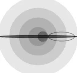
Definition 6. The tree of a formula ϕ, denoted τ (ϕ), is obtained from the syntactic tree of ϕ by labelling every edge e as follows: if e is the right (resp. left) outgoing edge of a binary connective, then it is labelled r (resp. l); otherwise it is labelled i. The graph of a formula ϕ, denoted G(ϕ), is the rooted graph obtained from τ (ϕ) by identifying the nodes of bound variables with their binders.
Example 2. Let Φ be the formula of Example 1. The tree and the graph of Φ are the following:
τ (Φ) = µX νY ∧ Y X i i r l i i G(Φ) = µX νY ∧ i i r l i i
Proposition 1. Let F = ϕα be an occurrence. Ifψβ is a
FL-suboccurrence ofF , then β = α.p, where p is a path of G(ϕ)
from the root to some noden, denoted NF(ψβ).
While defining the circular proof system, we will deal with sequences of occurrences related by →, that we call threads.
Γ, F ` ∆ Γ ` F, ∆ (Cut) Γ ` ∆ Γ ` ∆ ( ) Σ Γ ` Θ, ∆ F ≡ G (Ax) F ` G Γ ` ∆ (Wl) Γ, F ` ∆ Γ ` ∆ (Wr) Γ ` F, ∆ Γ, F ` ∆ Γ, G ` ∆ (∨l) Γ, F ∨ G ` ∆ Γ ` F, G, ∆ (∨r) Γ ` F ∨ G, ∆ Γ, F, G ` ∆ (∧l) Γ, F ∧ G ` ∆ Γ ` F, ∆ Γ ` G, ∆ (∧r) Γ ` F ∧ G, ∆
Fig. 1: Inference rules for propositional connectives. Γ, F [σX.F/X] ` ∆ (σl) Γ, σX.F ` ∆ Γ ` F [σX.F/X], ∆ (σr) Γ ` σX.F, ∆
Fig. 2: Fixed point rules for the µLK∞ proof system.
Definition 7. A thread of F is a sequence t = (Fi)i∈o, where
o ∈ ω + 1 s.t. F0= F and ∀i ∈ o, Fi→ Fi+1 or Fi= Fi+1.
Let t be the sequence (Fi)i∈o i.e., the sequence obtained by
forgetting the adresses of the formula occurrences of t. We denote by Inf(t) the elements of t that appear infinitely often in t.
A thread t starting from F can be seen as a path in the graph G(F ). Since t ⊆ FL(F ), Inf(t) is finite. The following proposition shows that Inf(t) admits a minimum.
Proposition 2. Let t = (Fi)i∈ω be a thread of F . The set
Inf(t) admits a minimum w.r.t. ≤, we denote it min(Inf(t)).
Example 3. Let t be the thread of Φε (from Example 1) that
goes to the right: t = Φε→ Ψi→?Ψiiri→?Ψiiriiri. . . We
have Inf(t) = {Ψ, Φ ∧ Ψ, Ψ} and min(Inf(t)) = Ψ. We are now ready to introduce our sequent calculus. 2) Circular proof system:
Definition 8. A sequent, written ∆ ` Γ, is pair of two finite
sets of pairwise disjoint occurrences. A pre-proof of µLK∞
is a possibly infinite tree, coinductively generated by the rules of Figures 1 and 2.
The disjointness condition on sequents ensures that two occurrences from the same side of a given sequent will never engender a common sub-occurrence. Note that if the disjointness condition is satisfied for the conclusion sequent of a pre-proof, then all its sequents satisfy it, as soon as occurrences of cut-formulas are appropriately chosen [11].
We sometimes write sequents of the form ϕε` ψεas ϕ ` ψ.
Pre-proofs are unsound: it is easy to derive the formula µX. X, which is semantically equivalent to ⊥, by applying
coinductively (µr) rule followed by ( ) rule. In order to obtain
proper proofs from pre-proofs, we add a validity condition that reflects the nature of our two fixed points.
Definition 9. A thread t is said to be a µ-thread (resp.
ν-thread) if min(Inf(t)) is a µ (resp. ν) formula. Let γ = (∆i`
t = (Fi)i∈ω is a right (resp. left) thread of γ if ∀i ∈ ω, Fi∈
Γi (resp. Fi∈ ∆i). The branch γ is said valid if it contains a
right ν-thread or a left µ-thread which is not stationary.
Definition 10. The proofs of µLK∞ are those pre-proofs in
which every infinite branch is valid.
This validity condition has its roots in parity games and is very natural for infinitary proof systems with fixed points. It is commonly found in deductive systems for modal µ-calculi: see [9] for a closely related presentation, which yields a sound and complete sequent calculus for linear-time µ-calculus.
In this work, we will be interested in a subsystem of µLK∞
whose proofs are finitely representable, we call it µLKω.
Definition 11. Two µLK∞ proofs Π, Θ are said to be equal
up to renaming, if there is a bijection b on adresses such that
the proof obtained from Π by replacing every occurrence ϕα
by ϕb(α) is Θ. A µLK
ω
proof is said to be circular if it has only finitely many sub-derivations up to renaming.
Definition 12. The circular proof system µLKωis the
restric-tion of µLK∞ to circular proofs.
The proofs of µLKωcan be represented by trees with loops.
For instance, the µLKωproof of > = νX. X is below, where
we indicated the loop using a symbol (?): (?) ` >ii ( ) ` ( >)i (νr) ` >ε (?)
The proof system µLKωis very close to the one in [9], that we
call µLKωDHL. The sequents of µLKωDHL are sets of formulas,
thus the proof search is trivial. This is not the case for µLKω.
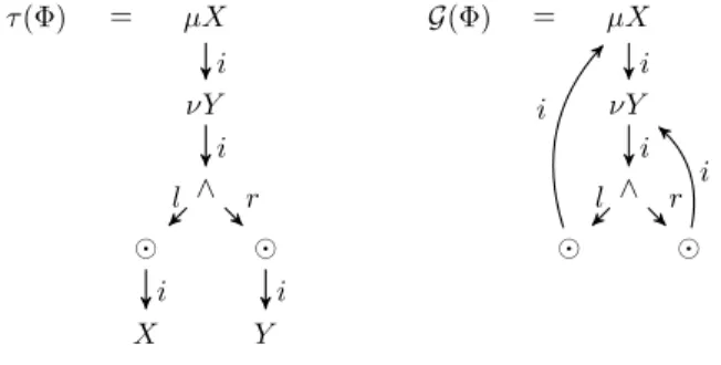
For instance, let ϕ = µX.νY.X ∨ Y and ψ = νY.ϕ ∨ Y its
unfolding. The µLKωDHLproof π of ϕ ∨ ψ (Fig. 3) is obtained
by applying bottom up all the possible logical rules. If we
apply the same rules in µLKω, we get the µLK∞ proof θ
(Fig. 3), which is not circular since the size of its sequents is unbounded. To get a circular proof, we have to apply some weakenings. But the choice of which formula to weaken is crucial, since a bad choice may lead to a non valid proof. For
instance, if we weaken the formula ψr, the obtained derivation
θ1(Fig. 3) is circular but does not satisfy the validity condition.
The good choice of weakening is the one that fires ϕl, yielding
the proof θ2 (Fig. 3). Proving a valid sequent in µLKω is
not trivial, since we have to do some clever choices to get derivations which are circular and valid.
3) Finitary proof system: We present now µLK, the
restric-tion of Kozen’s axiomatizarestric-tion for the modal µ-calculus to the linear time, written in a sequent calculus fashion.
Definition 13. The proofs of µLK are finite trees inductively generated from the rules of Figures 1 and 4.
In µLKω, µ and ν have the same rules, but their difference in
nature is reflected by the validity condition. In µLK, the rules for µ and ν are distinct; they are derived from the
Knaster-π = (?) ` ϕ ∨ ψ (µ),(ν),(ν) ` ϕ, ψ (∨) ` ϕ ∨ ψ (?) θ = .. . ` (ϕ ∨ ψ)lii, (ϕ ∨ ψ)ri (µ),(ν),(ν) ` ϕl, ψr (∨) ` (ϕ ∨ ψ)ε θ1= (?) ` (ϕ ∨ ψ)lii (µ),(ν) ` ϕl (W) ` ϕl, ψr (∨) ` (ϕ ∨ ψ)ε(?) θ2= (?) ` (ϕ ∨ ψ)ri (ν) ` ψr (W) ` ϕl, ψr (∨) ` (ϕ ∨ ψ)ε(?) Fig. 3: µLKωDHL, µLK ∞ and µLKω derivations of ϕ ∨ ψ F [S/X] ` S S ` Γ (µl) µX.F ` Γ Γ ` F [µX.F/X], ∆ (µr) Γ ` µX.F, ∆ Γ, F [νX.F/X] ` ∆ (νl) Γ, νX.F ` ∆ Γ ` S S ` F [S/X] (νr) Γ ` νX.F
Fig. 4: Fixed point rules for the µLK proof system.
Tarski characterization of µX.F as the least pre-fixed point of X 7→ F , and dually for νX.F .
Definition 14. A formula F is guarded if every bound variable of F appear under the scope of a connective.
In [6], it is shown that every formula if provably equivalent
to a guarded formula in µLKω, and this proof is constructive.
Proviso: If not otherwise stated all formulas are assumed
to be closed, guarded, > and ⊥ free. By earlier observations, this is not a restriction.
4) Relating the infinitary and the finitary proof systems: Finitary proofs can be easily transformed into circular ones, but giving an effective transformation from circular to finitary proofs is still an open problem. However, in [8] a condition
on µLKωproofs is given, which is sufficient to translate them
effectively into µLK ones. This condition is much involved and we do not need it here in all its generality. A weaker condition, presented below, will be used instead.
Definition 15. A µLKωderivation is thin if all the occurrences
of (σr) and (σl) are of the following form, i.e., there is no
context around the unfolded formulas: F [σX.F/X] ` ∆ (σl) σX.F ` ∆ Γ ` F [σX.F/X] (σr) Γ ` σX.F
Thin derivations are very close to thin refutations [6]. Proposition 3. If π is a thin proof of a sequent s, then it can
be transformed effectively into aµLK proof of s.
Proof. It suffices to notice that in a thin derivation every
valid branch is strongly valid (Definition 29 of [8]). Hence every thin proof is translatable (Definition 29 of [8]), by Proposition 30 of [8], it can be transformed effectively into a µLK proof of the same sequent.
III. ALTERNATING PARITY AUTOMATA ANDµ-CALCULUS
There is a fruitful relationship between µ-calculus and automata theory, at the core of which lies the equivalence between linear-time µ-calculus formulas and alternating parity automata (APW). This equivalence is always shown at a se-mantical level: every APW A can be encoded by a formula [A] such that M([A]) = L(A), and conversely for every formula
ϕ, there is an APW Aϕsuch that M(ϕ) = L(Aϕ). We show
in this section that beyond this semantical equivalence, there is also an equivalence at the level of provability, that is, ϕ and
[Aϕ] are provably equivalent in µLK. Lifting this semantical
equivalence to the provability level relies very precisely on
the encoding and the shape of the automaton Aϕ. That is
why we introduce our own encoding of automata in the µ-calculus, that respects the shape of the input automaton; and
our construction of Aϕ, which yields an automaton that sticks
the most to the structure of ϕ. This section is organized as follows: In III-A, we recall the model of APW and define in III-B our encoding of APW int the µ-calculus. Conversely, we construct in III-D for every µ-calculus formula an APW, and show that the encoding of this automaton is provably equivalent to the original formula in µLK. To do so, we need a technical tool, which is an alternative definition of µ-calculus semantics introduced in [12], that we recall in III-C.
A. Alternating parity word automata
Alternating parity automata over words (APW) are finite-state machines designed to accept or reject infinite words. The computation of an APW over an infinite word proceeds in rounds. At the beginning of every round, there are several copies of the APW in some position of the word, each of them in its own state. During a round, each copy splits up in several new copies, which are sent to the successor of the current position, and change their states, according to the transition function. Initially, there is only one copy of the APW, which is in the initial state; and which resides in the first position of the word. Every computation induces a tree, labelled with the states through which the copies of the automaton went during the computation; this tree is called a run and it witnesses the causality between a copy of the automaton and the new copies its yields. The acceptance or rejectance of a computation is defined via path conditions for the infinite branches of the run. Namely, every state is assigned a priority and an infinite branch of the run is accepting if the minimal priority occurring infinitely often is even; a run is accepting if all its infinite branches are accepting. We can see then the branching of runs as a universal non-determinism,; but APW support also existential non-determinism, in the sens that an automaton may have many possible computations over a single word. Formally APW are defined as follows.
Definition 16. An APW A is a tuple (Σ, Q, ∆, qI, c), where
Σ is an alphabet, Q is a finite set of states, ∆ ⊆ Q×Σ×2Qis
the transition relation, qI ∈ Q is the initial state and c : Q → ω
is the priority function, which assigns a priority to each state.
A run of A on a word u = (ai)i∈ω ∈ Σω is a labelled tree
such that: the label of the root is qI; and for every node v at
level n, if q is the label of v and if E is the set of labels of
the sons of v, then (q, an, E) ∈ ∆.
Example 4. Let A = ({a}, Q, ∆, p, c) be the APW where
Q = {p, q}, ∆ = {t1, t2, t3} where t1 = (p, a, {p}), t2 =
(p, a, {p, q}), t3 = (q, a, {p, q}) and c(p) = 1, c(q) = 2. ρ1
and ρ2are the beginning of two runs of A over aω.
ρ1= p p q p p q q p p p .. . .. . .. . .. . ρ2= p p q p p q p p q p q .. . .. . .. . .. . .. .
Definition 17. Let A = (Σ, Q, ∆, qI, c) and ρ be an infinite
word over Q. The word ρ is accepting if min { c(q) | q ∈ Inf(ρ) } is even. A run of A is accepting if all its branches (seen as words over Q) are. We say that A accepts the word u if there exists an accepting run of A on u. The language
of A is L(A) = { u ∈ Σω | A accepts u }. A language L
is recognized by A if L = L(A).
Non-deterministic automata are particular cases of alternat-ing automata where the existential non-determinism is allowed but not the universal one. We present below two classes of deterministic automata which are subclasses of APW: non-deterministic parity automata (NPW) and non-non-deterministic B¨uchi automata (NBW).
Definition 18. A NPW is an APW where the elements of the transition relation are of the form (p, a, {q}). A NBW is a
NPW (Σ, Q, ∆, qI, c) where the domain of c is {0, 1}. A state
q of a NBW is said to be accepting if c(q) = 0. We present
sometimes NBW as tuples of the form (Σ, Q, ∆, qI, F ) where
F is the set of accepting states.
For a non-deterministic automaton A = (Σ, Q, ∆, qI, c) we
can consider that ∆ is a subset of Q × Σ × Q and that the runs are infinite words over Q.
B. Encoding APW in theµ-calculus
The linear-time µ-calculus contains all the ingredients to encode APW : disjunction and conjunction to simulate exis-tential and universal non-determinism; least and greatest fixed points to encode odd and even states. To get a match between the language of an automaton and the models of the formula encoding it, we will consider automata over the alphabet
Σ = 2P where P is the set of atoms, whose elements will
simply be denoted by a, b, etc.
1) The encoding: We first show our encoding of the letters
of Σ in the µ-calculus.
Definition 19. Let a ∈ Σ. The encoding of a, denoted [a], is
Definition 20. Let A = (Σ, Q, ∆, qI, c) be an APW . A
run-section is a sequence Γ = ((qi, ti))0≤i≤n of pairs in Q × ∆
s.t. q0 = qI and ∀i ≤ n, ∃ai, Ei st. ti = (qi, ai, Ei) and
∀i < n, qi+1 ∈ Ei. We say that Γ enables a state q if q ∈ En.
Definition 21. Let A = (Q, qI, ∆, c) be an APW . We assume
a collection of variables (Xq)q∈Q. We define the formula [q]Γ
encoding the state q ∈ Q under the run-section Γ, as follows:
[q]Γ = X q if (1) Γ = Γ0, (q, t), (q1, t1), . . . , (qn, tn) and (2) qi6= q, c(qi) ≥ c(q) for all 1 ≤ i ≤ n, [q]Γ = σX q. W a∈Σ,t=(q,a,E)∈∆ [a] ∧ V p∈E [p]Γ,(q,t) otherwise
with σ = ν iff c(q) is even.
We finally set [A] = [qI]∅.
The encoding starts from the initial state and traverses the
automaton, encoding every state q by a fixed point µXq, if
q is a state with an odd priority and νXq otherwise. The
environment Γ remembers the states that have been visited from the initial state to the current state. If the current state q has been seen before (and if the states seen since the last time q was visited have bigger priorities) then we encode it by its
corresponding variable Xq, which ensures that the algorithm
of encoding will halt at some point.
Example 5. The encoding of A of Example 4 is the formula:
[A] = µXp.([a]∧ Xp)∨([a]∧ (νXq.[a]∧ Xq∧ Xp)∧ Xp)
A key ingredient in this encoding is the side condition of the first case of the definition. The aim of this condition is to bridge the gap between the acceptance condition on runs of the automaton and the validity condition on threads. The latter is almost a parity condition, but with a parity ordering corresponding to the subformula ordering. To obtain a match between the two orderings, we need to control the formation of cycles (see Example 16 in [8]).
Although not necessary for the completeness proof, we prove the following proposition, which shows that the lan-guage of an automaton and the models of its encoding are equal.
Proposition 4. For any APW A, M([A]) = L(A)
Proof. For this proof we use definitions and result from
Section III-C. We show that the automaton A and the formula [A] have the same language ie. L(A) = L([A]).
We show first that L([A]) ⊆ L(A). Let u ∈ L([A]) and let β be an accepting branch of Π([A]) that induces u. Let
s1s2. . . be the sequence of conclusions of rules in β. Every
si is of the from Ci, {JqkK
Γk}
i0≤k≤ili where Ci = C(ui).
This branch induces easily a run ρ of A over u, where at
every level i of ρ, the set of nodes labels is {qk}i0≤k≤ili.
Every branch of ρ is a run-branch of a thread t of β. Since
β is accepting, every thread t of β is a ν-thread, thus by Proposition 7 every branch of ρ is valid, hence ρ is valid.
We show the other direction L(A) ⊆ L([A]) by using a
similar argument: to every valid run of Aϕ over a word u,
one can find an accepting branch of Π(ϕ) that induces the word u.
By Proposition 8, L(ϕ) = M(ϕ), which concludes the proof.
2) FL-suboccurrences of the encoding: The µLKω proofs
involving a formula [A], that we will deal with later, will decompose [A] into its FL-suboccurrences. To simplify the manipulation of these FL-suboccurrences, we introduce in this section same handy notation, then we relate the threads of [A] , which are sequences of FL-suboccurrences of [A], to the runs of the automaton A.
Definition 22. Let Γ = ((qi, ti))0≤i≤nbe a run-section of the
APW A, and q a state enabled by Γ. Let p be the path in the
graph of [A] that visits successively the nodes labelled σXqi,
according to the transitions ti, and ends with the node labelled
σXq. The address of (Γ, q), denoted αΓ,q, is the label of p.
Example 6. Let A be the APW of Example 4. To simplify the presentation of the formula graphs, we merge the chain of nodes of the following shape into one node labelled [a] ∧ :
∧ ∧ [a] n0 n1 r l r l i i [a] ∧ n1 n0 lri ri
The graph of the encoding of A is the following: νXp ∨ [a] ∧ [a] ∧ µXq [a] ∧ i l r ri lri ri i lri ri
The run-section Γ = (p, t2), (q, t3) enables the state q, its path
is the dashed one. The address αΓ,q is irlriilri.
Definition 23. Let Γ be a run-section of A, and q a state
enabled by Γ. We denote by JqK
Γ the FL-suboccurrence of
[A] at the address αΓ,q, i.e., the occurrence ϕαΓ,q such that:
[A]ε→?ϕαΓ,q.
Example 7. Let Γ be the run-section of Example 6. We have JqK
Γ= (µX
q.[b] ∧ Xq∧ [A])αΓ,q.
Remark 1. We have chosen the notationJqK
Γ because of the
[q]Γ. Indeed, one can show that
JqK
Γis obtained by substituting
iteratively the free variables of [q]Γ by their binders in [A].
Remark 2. The formulas JqK
Γ are fixed point formulas.
Conversely, all the fixed point FL-subformulas of [A] are of
the formJqKΓ where Γ, q is a run-section.
The following proposition will be very useful for further
proofs. It shows that contrarily to [q]Γ, no case analysis on Γ
and q is required to figure out the shape of JqKΓ.
Proposition 5. Let A be an APW and JqKΓ a
FL-suboccurrence of[A]. The top-level connective ofJqKΓisσXq.
and we have: JqK Γ → _ t=(q,a,E)∈∆ [a] ∧ ^ p∈E JpKΓ,(q,t)
Using Proposition 5, we can derive the following rule, which
mimics automata transitions in the proof system µLK∞.
Proposition 6. Let A be an APW of transition relation ∆, q
be state ofA and Γ a run-section. For every set of occurrences
Θ, the following rule is derivable using a thin derivation:
{[a], {JpKΓ,(q,t)} p∈E` Θ}t=(q,a,E)∈∆ JqK Γ` Θ Proof. Since JqK Γ → W t=(q,a,E)∈∆ [a] ∧ V p∈E JpK Γ,(q,t) , one
can derive the following: [a], { JpKΓ,(q,t)} p∈E` Θ (∧l) [a] ∧ V p∈E JpKΓ,(q,t)` Θ t=(q,a,E)∈∆ (∨l) W t=(q,a,E)∈∆ [a] ∧ V p∈E JpKΓ,(q,t)` Θ (σl) JqK Γ` Θ
Notice that this is a thin derivation.
Now we relate the threads of the formula encoding an automaton A to the run branches of A. For that, we define the run-branch corresponding to a thread of [A] as follows: Definition 24. Let A be an APW and t be a thread of [A]. Let (JqiK
Γi)
i∈ω be the sequence of fixed point occurrences
appearing in t. The run-branch of t is ρ(t) := (qi)i∈ω.
It is easy to see that the run-branch of a thread is indeed a branch in a run of A.
Proposition 7. Let A be an APW , c be its priority function.
A thread t of [A] is a ν-thread iff ρ(t) is a valid.
C. Operational semantics
Our goal now is to extract an APW from every µ-calculus formula. In [12], an alternative definition of formulas se-mantics is presented, equivalent to Definition 2, but with the advantage that it makes formulas look like automata, checking whether words over Σ are models or not. This is exactly what we need to achieve our goal. Their definition being introduced
for the modal µ-calculus, we specialize it to the linear time case.
Definition 25. We call constraint any set of literals. The constraint of a letter a ∈ Σ, denoted c(a), is the constraint
a ∪ {p⊥ | p /∈ a}. A letter a satisfies a constraint c, and we
write a |= c, iff c ⊆ c(a).
Definition 26. Let F be an occurrence. The F -derivation is a
µLK∞ derivation of conclusion F ` obtained by applying all
the possible logical rules (µ, ν, ∨, ∧), except for the rule, to F and its sub-occurrences, until reaching sequents of the form C, ∆ `, where the set C obtained by forgetting the addresses of C, is a constraint. The set of successors of F , denoted S(F ), is the set of premises of the F -derivation.
Notice that the F -derivation is finite, because F is guarded. Remark 3. There are many possible F -derivations for a given occurrence F , differing only by the order of application of the logical rules. They all share the same set of premises and the same structure of threads. We choose any representative of this class of derivations to be the F -derivation.
Example 8. Let F = νX.p ∧ (( X)α∨ G) ∧ ( X)β, where
G = µY.q ∧ ( Y )γ. The F -derivation is the following:
p, ( F )α, ( F )β` p, q, ( G)γ, ( F )β` (µ),(∧l) p, G, ( F )β` (∨) p, ( F )α∨ G, ( F )β` (ν),(∧),(∧) F `
We sometimes write an F -derivation as a rule named F : p, ( F )α, ( F )β` p, q, ( G)γ, ( F )β`
(F )
F `
Recall that if F is an occurrence and β an address, Fβ is the
relocation of F in β (Definition 4). Recall also that we made the choice not write explicitly the addresses of atoms.
Definition 27. Let ∆ := {Fi}1≤i≤n be a set of occurrences.
The ∆-derivation is a µLK∞ open derivation of conclusion
∆ ` obtained by applying successively, and for all 1 ≤ i ≤ n,
the Fi-derivations until reaching sequents of the form C, ∆ `
where C is a constraint. The set of successors of ∆, denoted S(∆), is the set of premises of the ∆-derivation.
Remark 4. Here again, there are many possible ∆-derivations
but they differ only by the order where Fi -derivations are
applied. They all share the same structure of threads and the same set of premises.
Example 9. Let F be the occurrence of Example 8 and H =
νX.r ∧ ( X)δ. The {F, H}-derivation is the following:
p, r, ( F )α, ( F )β, ( H)δ` (H) p, ( F )α, ( F )β, H ` p, q, r, ( G)γ, ( F )β, ( H)δ` (H) p, q, ( G)γ, ( F )β, H ` (F ) F, H `
p, r, ( F )α, ( F )β, ( H)δ` p, q, r, ( G)γ, ( F )β, ( H)δ` ({F, H})
F, H `
Definition 28. We define Π(∆) to be the µLK∞ pre-proof
of conclusion ∆ `, obtained by applying coinductively the following scheme: Π(∆) = Π(∆1) ( ) C1, ∆1` . . . Π(∆n) ( ) Cn, ∆n` (∆) ∆ `
Example 10. Let ϕ = µX.νY. ((p ∧ Y ) ∨ X), ψ = νY. ((p ∧ Y ) ∨ ϕ) and δ = (p ∧ ψ) ∨ ϕ. The derivation Π(` δ) is:
(†) δlii` ( ) p, ( δ)li` (†) δriii` ( ) ( δ)rii` (δε) (†) δε`
Notice that Π(` F ) is not a µLK∞proof in general, because
it dos not always satisfy the validity condition. This is not a problem, since the goal is to use it only as a support to compute the set of models of F .
Definition 29. Let β be a branch of Π(` F ) and
((Ci, ∆i))i∈ω be the sequence of the conclusions of the
rules in β. A word u = (ai)i∈ωis said to be induced by β iff
∀i, ai|= Ci. The branch β is said to be accepting if it contains
no µ-thread. The language of F , denoted L(F ), is the set of words induced by the accepting branches of Π(` F ). Example 11. If P = {p} then Σ = {a, b} where a = ∅ and
b = {p}. The language of δ from Example 10 is {a, b}?.bω.
The use of automata-theoretic vocabulary is due to the fact that we can see an occurrence F as a sort of APW. Indeed, when we put F in the left hand-side of the sequent, the left disjunction rules become branching, and we can see each branch as a non-deterministic choice of a run, while the conjuction rule is non branching and we can see the application of conjuction rule as constructing an alternating run. Hence, every infinite branch of Π(` F ) can be seen as a run of an alternating automaton. Moreover, the acceptance condition of a branch of Π(` F ) recalls the parity condition for APW. We will make this remark more precise in the next sections. Proposition 8 ([12]). For every formula F , L(F ) = M(F ). D. From Formulas to APW
In this section, we exploit the intuitions and tools developed in Section III-C to extract from every µ-calculus formula ϕ an
APW Aϕ. We show not only that ϕ and [Aϕ] are semantically
equivalent, but also that [Aϕ] ` ϕ is provable in µLK.
1) APW of a formula: Let us give an outline of the
construction of the APW Aϕ corresponding to a formula ϕ.
Definition 29 suggests that we can see the FL-suboccurrences of ϕ as the states of an APW, whose transitions are given by the F -derivations. For instance, the derivation Π(δ) of
Example 10 suggests that the set of states of Aδ is {δ} and its
transition relation is {(δ, a, δ), (δ, b, δ)}. To assign a priority to
the state of Aδ, we have to look at the formulas hidden in the
δ-derivation. Indeed, what makes the leftmost branch of Π(δ) accepting is the formula ψ hidden in the δ-derivation. Hence we want the priority of δ to be that of ψ, thus to be even. But
if we do so, the word aω, induced by the rightmost branch
of Π(δ), will be accepted also by Aδ. The rightmost branch
of Π(δ) is not accepting because the minimum of its thread is ϕ. To get an automaton that accepts exactly the models of δ, one should have two copies of the state δ, one with
an odd priority corresponding to ϕ, we denote it δϕ and the
other with an even priority corresponding to ψ, we denote
it δψ. More generally, the states of the alternating automaton
corresponding to a formula will be pairs of formulas, written as
δψ, where δ is morally the state and ψ is a formula containing
the priority information.
To generalize this idea, we have to ensure that in an F -derivation, every thread linking F to an occurrence appearing in a premise of this F -derivation admits a minimal formula: Proposition 9. Let s be a successor of F and G ∈ s. The
thread of the F -derivation, linking F to G, has a minimal
formula ψ wrt. the subformula ordering.
We writeF s,ψ→ G as a shortcut for: “The minimum of the
thread linkingF to G in the F -derivation is ψ”.
To show this result, we need the notion of straight threads:
Definition 30. Let F be an occurrence and t = (Fi)1≤i≤k be
a thread. For all 1 ≤ i ≤ k, let ni= NF(Fi) (Proposition 1).
Recall that ni are also nodes of τ (F ). The thread t is said to
be a straight thread if the node ni+1is the son of niin τ (F ).
It is not difficult to show, by induction on k the following: Proposition 10. If t is a straight thread then t admits a
minimumw.r.t. ≤.
Proof of Proposition 9. It suffices to notice that the thread t
linking F to G is a straight thread. By Proposition 10 it admits a minimal formula wrt. the subformula ordering.
The following proposition is traightforward. It shows that the minimum of the thread linking F to a formula occurrence G appearing in one of its successors does not change if we relocate F .
Proposition 11. Let ϕαbe an occurrence ands ∈ S(ϕα). We
have:
• The sequent s is of the form s = {(ϕi)α.αi}0≤i≤n.
• For every address β, s0:= {(ϕi)β.αi}0≤i≤n∈ S(ϕβ),
• and ∀i ≤ n if ϕα
s,ψ
→ (ϕi)α.αi thenϕβ
s,ψ
→ (ϕi)β.αi.
We define in the following, for every formula ϕ, a function
pϕ that assigns to every FL-subformula of ϕ an integer,
in a way that respects the subformula ordering and that is compatible with the nature of fixed-point formulas.
Definition 31. Let ϕ be a formula and let pϕ : F L(ϕ) → ω
be a function such that:
• If ψ ≤ δ then pϕ(ψ) ≤ pϕ(δ).
The function pϕ is not unique but we can fix one arbitrarily.
The function pϕwill be used to assign priorities to the states
of the APW corresponding to the formula ϕ.
Definition 32. The APW associated to ϕ, denoted Aϕ, is
the tuple (Σ, Q, qI, ∆ϕ, c) where the set of states is Q =
{δγ | δ, γ ∈ F L(ϕ)}, the initial state is q
I = ϕϕ, the
priority function is defined by c(δγ) = pϕ(γ) and the transition
relation ∆ϕ is defined as follows: (ψδ, a, E) ∈ ∆ϕ iff there
is s = (C, ∆) ∈ S(ψε) such that a |= C and:
γσ∈ E ↔ ∃( γβ) ∈ s such that ψε
s,σ
→ γβ
Notice that the choice of qI as ϕϕ is arbitrary, one could
choose any state of the form ϕδ.
Proposition 12. We have L(Aϕ) = M(ϕ).
We show that the automaton Aϕ and the formula ϕ have
the same language ie. L(Aϕ) = L(ϕ).
We first show that L(ϕ) ⊆ L(Aϕ). Let u ∈ L(ϕ) and let β
be an accepting branch of Π(` ϕ) that induces u. Let (si)i∈ω
be the sequence of conclusions of rules in β. For every
i ∈ ω, si is of the from Ci, ∆i where Ci is a constraint.
We construct in the following a run ρ of Aϕ over u, level by
level, starting from the root. In this construction, we keep the
following invariant: for every i ∈ ω, if ∆i= {(δj)αj}1≤j≤n,
then there exists a set of formula {ψj}1≤j≤nsuch that the set
of nodes labels at level i in ρ is {δψj
j }1≤j≤n.
Level 1: We label the root of ρ by ϕϕ. The sequent ∆
1
is of the form {(δj)αj}1≤j≤n. For every j ≤ n, there exists
ψj such that ϕε
s1,ψj
→ ( δj)αj, we add then to the root a son
labelled δψj
j . Our invariant is satisfied for level 1.
Level i → Level i+1: If ∆i = ((δk)αk)1≤k≤n then si+1
is of the form si+1 = ∪
1≤k≤nvk, where vk ∈ S((δk)αk), for
every k ≤ n. Let w be a node of level i, labelled δψk
k . For
every occurrence ( γ)α in vk, there exists a formula ψ such
that (δk)αk
vk,ψ
→ ( γ)α, we add to w a son labelled γψ. Here
again, our invariant is satisfied for level i + 1.
The run ρ is valid. Indeed, let b = (δψi
i )i∈ω be a branch
of ρ. We will show that b is valid using the validity of the
branch β of Π(` ϕ). By construction one has that δψ0
0 = ϕϕ
and there exists a sequence of addresses (αi)i∈ω such that for
every i ∈ ω we have (δi)αi ∈ ∆i. Moreover, the thread linking
(δi)αi to (δi+1)αi+1 in Π(` ϕ), that we denote ti, satisfies the
following property: min(ti) = ψi+1. Let t = t0t1. . . be the
thread of Π(` ϕ) obtained by the concatenation of the threads
{ti}i∈ω. Let k, l ∈ ω such that the subthread tk. . . tl of t
contains all the elements of Inf (t). One has also that the
subsequence δψk
k , . . . , δ ψl+1
l+1 of b contains all the elements of
Inf (b). One has:
min(Inf (t)) = min(tk. . . tl)
= min(min(ti))k≤i≤l
= min(ψi)k≤i≤l
Since the branch β is accepting, min(ψi)k≤i≤lis a ν-formula.
Moreover, if c is the priority function of Aϕ and pϕ the
auxiliary function used to define it (Definition 31), then we have: min(c(Inf (b))) = min(c(δψk k ), . . . , c(δ ψl+1 l+1 )) = min(pϕ(ψk), . . . , pϕ(ψl+1)) † = pϕ(min(ψi)k≤i≤l)
(†) Since the function pϕ is monotonic
Since min(ψi)k≤i≤l is a ν-formula, one has that
pϕ(min(ψi)k≤i≤l) is even, hence the branch b is valid. We
conclude that ρ is valid and u ∈ L(Aϕ).
We show the other direction L(Aϕ) ⊆ L(ϕ) using a similar
argument: to every valid run of Aϕ over a word u, we can
find an accepting branch of Π(ϕ) that induces u.
By proposition 8, L(ϕ) = M(ϕ), which concludes the proof.
2) [Aϕ] ` ϕ in µLK: We show that there is a proof of
[Aϕ] ` ϕ in µLK. The idea is to construct a thin proof of
this sequent in µLKω, and using Proposition 3, to transform
it into a proof in µLK. Since ϕϕis the initial state of Aϕ, we
have that [Aϕ]ε=Jϕ
ϕ
K
∅, hence our goal is to show that the
sequentJϕϕ
K
∅` ϕ
εhas a thin µLKωproof. To get this result,
we need to generalize our statement and to look for proofs of
sequents having the formJψδ
K
Θ` ψ
α, where ψδ is a state of
Aϕ, Θ a run-section and α an address. Using Proposition 6,
we decompose the left-hand side of such sequents and get the following derivation: {[a], { Jγσ K Θ,(ψδ,t)} γσ∈E ` ψα}t=(ψδ,a,E)∈∆ ϕ Jψ δ K Θ` ψ α
Each premise of this derivation corresponds to a transition
in ∆ϕ, and by construction of ∆ϕ, every such transition
corresponds to a successor s ∈ S(ψε). To get a proof of
such premise which is thin, we have to apply weakenings at some points, so that when unfolding the fixed points, their context will be empty. The choice of these weakenings will be guided by this successor s in a sense that we will clarify in the following. But first, let us look closely into the notion of the successor of a formula.
If s is the successor of ψε, then for every F ∈ s, the address
of F induces a path in the tree of ψ. When we collect all the paths induced by the formula occurrences of s, we get a sub-tree τ (s) of τ (ψ), as illustrated by the following example. Example 12. Let ψ = µX.(( X ∧ p) ∨ δ) ∧ (q ∨ δ) where
δ = νY. Y . Let s = p, ( ψ)α, ( δ)β be the successor of
ψε where α = illl and β = irr. The paths of τ (ψ) induced
by the formula occurrences of s form a tree τ (s) indicated by the dashed lines below:
τ (ψ) = µX ∧ ∨ ∨ ∧ p X τ (δ) q τ (δ) i l r l r l r i r l i i
Any node n of τ (s) satisfies the following properties:
• If n is labelled , the son of n does not belong to τ (s).
• If n is labelled ∧, the two sons of n belong also to τ (s).
• If n is labelled ∨, exactly one son of n belongs to τ (s).
A successor s ∈ S(F ) induces a function that chooses, for every suboccurrence of F which is a disjunction, one of its
disjuncts; we call this function Cs.
Definition 33. Let s = {(δi)αi}1≤i≤n be the successor of an
occurrence F = ϕα. For all αi, there is pi st. αi= α.pi.
The choice of s is a partial function on occurrences defined
as follows. For all i, and for every address a v pi such that
the node of τ (ϕ) at the address a is labelled ∨, we set:
Cs((ϕ ∨ ψ)a) = ϕa.l if a.l v pi,
= ψa.r otherwise.
Example 13. In Example 12, we have: Cs(( ψ∧p)∨ δ)il) =
( X ∧ p)ill and Cs((q ∨ δ)ir) = ( δ)irr.
Using this function, we define the derivation Πs(Γ ` F ). In
this derivation of conclusion Γ ` F , we apply only right rules, and whenever we meet a right formula which is a disjunction,
we apply (∨r) rule followed immediately by a weakening, that
keeps only the formula chosen by Cs. Doing so, we obtain a
derivation which is thin, since we keep the invariant that we have exactly one right formula along the derivation.
Definition 34. Let F be an occurrence, s ∈ S(F ) and Γ be
a set of occurrences. The derivation Πs(Γ ` F ) is the µLKω
derivation of conclusion Γ ` F obtained by applying only the following rules: Γ ` F Γ ` G (∧r) Γ ` F ∧ G Γ ` F [σX.F/X] (σr) Γ ` σX.F Γ ` Cs(F ∨ G) (Wr) Γ ` F, G (∨r) Γ ` F ∨ G
Example 14. We show in the following the derivation Πs(`
ψε), where s and ψ are defined in Example 12.
` ( ψ)illl ` p (∧r) ` ( ψ ∧ p)ill (∨r),(Wr) ` (( ψ ∧ p) ∨ δ))il ` ( δ)irr (∨r),(Wr) ` (q ∨ δ)ir (∧r) ` (( ψ ∧ p) ∨ δ) ∧ (q ∨ δ))i (µr) ` ψε
The following proposition is traightforward.
Proposition 13. Let F be an occurrence, s ∈ S(F ) and Γ be a set of occurrences.
• Πs(Γ ` F ) is a thin derivation.
• The premises ofΠs(Γ ` F ) are {Γ ` G | G ∈ s}.
• IfΓ ` G is a premise of Πs(Γ ` F ) and if F
s,ψ
→ G then
the minimum of the thread linkingF to G in Πs(Γ ` F )
isψ.
Proposition 14. Let ϕ be a formula and ψδ be a state of
Aϕ. The following rule is derivable in µLKω using a thin
derivation: {Jγσ K Θ,(ψδ,t) ` γα.β}s∈S(ψ ε),γβ∈s,ψε s,σ → (γ)β (◦) Jψ δ K Θ` ψ α
And the minimum of the thread linkingψα toγα.β isσ.
Proof. We already noticed that the following rule is derivable:
{[a], { Jγσ K Θ,(ψδ,t) }γσ∈E` ψα}t=(ψδ,a,E)∈∆ ϕ Jψ δ K Θ` ψ α
By definition of ∆ϕ, we have that (ψδ, a, E) ∈ ∆ϕiff there is
s = (C, ∆) ∈ S(ψε) s.t. a |= C and if the following holds:
γσ∈ E ↔ ∃( γβ) ∈ s such that ψε
s,σ
→ γβ
To justify a premise corresponding to a transition t =
(ψδ, a, E), we set Γ = [a], {
Jγ
σ
K
Θ,(ψδ,t)}
γσ∈E and apply
the derivation Πs(Γ ` ψα):
{Γ ` pη}pη∈C {Γ ` (γ)α.β} (γ)β∈s
(Πs(Γ ` ψα))
Γ ` ψα
To justify a premise Γ ` pη, we notice that since a |= C, we
have C ⊆ a, thus [a] is of the form [a] = p ∧ G. We then apply the following derivation:
(∧l), (Ax)
[a] ` F
(Wl)
Γ ` F
Now we want to justify a premise Γ ` (γ)α.β. If ψε
s,σ
→
γβ, then γσ∈ E, we can thus apply the following:
Jγ σ K Θ,(ψδ,t) ` γα.β ( ) Jγ σ K Θ,(ψδ,t) ` (γ)α.β (Wl) Γ ` (γ)α.β
The obtained derivation is thin and by Proposition 13, the
minimum of the thread linking ψα to γα.β is σ.
The premises of the derived rule (◦) have the same shape as its conclusion. If we iterate this derivation starting from
[Aϕ] ` ϕ (which is Jϕ ϕ K ∅ ` ϕ ε) we obtain a thin µLKω pre-proof.
We show that this pre-proof is actually a proof. Using Proposition 3, we can transform this thin proof into a µLK
proof of [Aϕ] ` ϕ.
Theorem 1. We can construct a µLK proof of [Aϕ] ` ϕ.
Proof. Let c be the priority function of Aϕ and pϕ
Jϕ
ϕ
K
∅. Let π be the µLK∞ pre-proof obtained by applying
coinductively the derivation (◦) of Proposition 14. It is not
dif-ficult to see that π is a thin µLKωpre-proof. We show now that
π is µLKω proof, i.e., that is satisfies the validity condition.
Let γ be an infinite branch of π and (Jψδi
i K
Θi ` (ψ
i)αi)i∈ω
be the sequence made of the conclusions of the derivation ◦.
In γ, there is exactly one right thread tr and one left thread
tl. The thread tl is a thread of [A]. Let ρ(tl) be the
run-branch of tl (Definition 24). Let v = (δi)i∈ω. we have that
ψδ∈ Inf (ρ(t
l)) ⇔ δ ∈ Inf (v). Hence we have that:
(?)
min({c(ψδ) | ψδ ∈ Inf (ρ(t
l))})
= min({pϕ(δ) | ψδ ∈ Inf (ρ(tl))})
= min({pϕ(δ) | δ ∈ Inf (v)})
In another hand, since the minimum of the thread linking ψi
to ψi+1 in γ is δi, we have:
(†) min({ψ | ψ ∈ Inf (tr)})
= min({δ | δ ∈ Inf (v)})
There is two possible cases: either tl is a µ-thread, thus γ is
valid; or tl is a ν-thread then by Proposition 7 the run-branch
ρ(tl) is accepting, then, by (?), min({pϕ(δ) | δ ∈ Inf (v)})
is even. By definition of pϕ, min({δ | δ ∈ Inf (v)}) is a
ν-formula, thus by (†), tr is a ν-thread, which means that γ is
valid.
Theorem 1 is the step I of our proof of completeness.
Actually, we can show also that ϕ `µLK [Aϕ] in the same
way.
IV. REFLECTING AUTOMATA EQUIVALENCES IN THE LOGIC
It is well known that APW, NPW and NBW are three equivalent models of automata This result is usually shown by exhibiting automata transformations that convert an automaton of a given model into an automaton in the other models, by preserving the language. In this section, we recall the automata transformations that will be used for the proof of completeness, and show that the transformations provide, via the encoding, provably equivalent formulas.
A. From APW to NPW
We recall the construction that transforms an APW A into an NPW P such that L(P) = L(A). In a second step, we show that the sequent [P] ` [A] in provable µLK.
1) Non-determinization: We recall in this section the
op-eration of non-determinization, that transforms an APW into a NPW with the same language. In [13] this construction is presented for automata over trees, we specialize it here for
automata over words. We fix an APW A = (Σ, Q, ∆, qI, c).
The key ingredient to non-determinize APW is to simplify their runs. Runs of APW may be non-uniform in the sense that two nodes at the same level and labelled with the same state, may have different sets of successors. For instance, in the
run ρ2 of Example 4, the two nodes at level 2 and labelled p
have as sets of successors {p} and {p, q} respectively. On the contrary, we call uniform a run such that: all nodes at the same level and with the same labels have the same set of successors.
Uniform runs are sufficient to compute the languages of APW [13]: u ∈ L(A) iff there is a valid uniform run of A over u.
In a uniform run, every level can be described by a func-tion that maps a state to the set of its successors: uniform runs can be described by sequences of such functions. For
instance, the run ρ1 of Example 4 can be seen as a sequence
f0f1f2. . . where f0(p) = {p, q}, f1(p) = {p, q}, f1(q) = q,
f2(p) = {p, q}, f2(q) = q, etc. We call these functions
choice functions. The interest of using uniform runs instead of arbitrary runs is that we went from runs having a tree structure to runs with a structure of words (sequences of choice functions), that we will be able to synchronize with Σ-words.
Definition 35. A choice function is a function σ : Q → 2Q.
The set of choice functions is denoted S. Notice that S is
finite.The auxiliary alphabet of A is Σaux = {(a, σ) ∈ Σ ×
S | (p, a, σ(p)) ∈ ∆}.
Two sequences can be extracted from a word U over Σaux:
the first is a word u over Σ obtained by projection on the first components of U , and the second is a sequence of choice functions obtained by projection on the second components of U . This latter sequence describes a uniform run of A over u.
Definition 36. Let U = ((ai, σi))i∈ω ∈ (Σaux)ω. The run
associated to U is a labelled tree such that: the root is labelled
qI; and for every node v at level n, if q is the label of v then
each son of v is labelled with one of the sates of σn(q). Notice
that τ is a uniform run of U over the word (ai)i∈ω.
Definition 37. The language L ⊆ (Σaux)ω is the auxiliary
language of A iff ∀U ∈ L, the run associated to U is accepting (w.r.t. the acceptance condition of A). We denoted
it by Laux(A).
The idea of the non-determinization is to exhibit a deter-ministic parity automaton (DPW) recognizing the auxiliary language of A. Intuitively, this is possible since all the
information of alternation is explicit in the Σaux-words, hence
we do not need an alternating automaton to recognize it. One this is done, we erase the choice functions from the transition structure of this automaton, to get an NPW recognizing the language of A.
Proposition 15. For very APW we can construct effectively a NPW recognizing the same language.
Proof sketch. Let A = (Σ, Q, ∆, qI, c) be an APW. We
construct a NPW recognizing the language of A in two steps.
I. Construct a DPW D = (Σaux, Qd, qd
I, ∆
d, cd) such that
L(D) = Laux(A). This is done in 4 steps:
a) Construct anAP W recognizing Laux(A): Let A
1=
(Γ, Q, ∆1, qI, c) be the APW where:
∆1= {(p, (a, σ), E) | (p, a, E) ∈ ∆ and σ(p) = E}
The language of A1 is Laux(A). Notice that for every
Σaux-word, there is only one possible run over A
b) Construct a N P W recognizing the complement of
Laux(A): Let A
2 = (Γ, Q, ∆2, qI, c2) be the APW
where c2(q) = c(q) + 1 and:
∆2= {(p, A, q) | ∃E, (p, A, E ∪ {q}) ∈ ∆1}.
The language of A2 is the complement of Laux(A).
Indeed, R is a run of A2 over U iff R is a path in the
unique run of A1over U . Since we shifted the priorities
in A2, R is a valid run of A2over U iff R seen as a path
in the run of A1 over U is not valid. Thus, U ∈ L(A2)
iff U /∈ L(A1).
c) A DP W recognizing the complement of
Laux(A): Determinize A
2 to get a DP W
A3 = (Γ, Q3, ∆3, pI, c3), using a determinisation
technique (Safra construction for example).
d) A DP W recognizing Laux(A): Let A
4 =
(Γ, Q3, ∆3, pI, c4) where c4(q) = c3(q) + 1. One has
L(A4) = Laux(A).
II. Let P = (Σ, Qd, qId, ∆0, cd) where ∆0 =
{(d, a, d0) | ∃σ, (d, (a, σ), d0) ∈ ∆d}. One has
L(P) = L(A).
2) [P] `µLK [A]: Let A be an APW automaton and P
be the NPW obtained in the proof of Proposition 15. In this section we show that [P] ` [A] has a proof in µLK. For that
purpose, we build a thin µLKω proof of this sequent, which
gives us a µLK proof by Proposition 3. We use in this section
the notations of the proof sketch of Proposition 15. Since qI
and qdI are the initial states of A and P respectively, we have
that [A]ε=JqIK
∅and [P]
ε=Jq
d IK
∅. Our goal is then to show
that Jq
d IK
∅ `
JqIK
∅ is provable with a thin µLKω
proof. To do so, we need to generalize this statement, and to look for
proofs of sequents having the formJdKΘ`
JqK
Υ, where d and
Θ (resp. q and Υ) are a state and a run-section for P (resp. A). We show the following lemma:
Lemma 1. The following rule is derivable in µLKω using a
thin derivation: {Jd 0 K Θ,(d,t)` Jq 0 K Υ,(q,T )} (d,(a,σ),d0)∈∆d,q0∈σ(q) (→) JdK Θ` JqK Υ Where t = (d, a, d0) and T = (q, a, σ(q)).
Proof. We have t = (d, a, d0) ∈ ∆0 iff ∃(a, σ) ∈ Σaux such
that (d, (a, σ), d0) ∈ ∆d. Using Proposition 6, we can derive
the following, where t = (d, a, d0):
{[a], Jd 0 K Θ,(d,t)` JqK Υ} (q,(a,σ),d0)∈∆d JdK Θ` JqK Υ
Now we have to justify every premise of this derivation
corre-sponding to a transition (q, (a, σ), d0) ∈ ∆d. By Proposition 5:
JqK Υ → W a∈Σ,(q,a,E)∈∆ [a] ∧ V q0∈E Jq0 K Υ,q
Since (a, σ) ∈ Σaux, then T := (q, a, σ(q)) ∈ ∆. If we set
Γ := [a], Jd0KΘ,(d,t), we can the derive the following:
( Jd 0 K Θ,(d,t)` Jq 0 K Υ,(q,T ) ( ) Γ ` Jq0KΥ,(q,T ) ) q0∈σ(q) (Ax) Γ ` [a] (∧r) Γ ` [a] ∧ V q0∈σ(q) Jq0 K Υ,(q,T ) (σr), (∨r),(Wr) Γ `JqKΥ
The premisses of the derivation (→) have the same shape as its conclusion. If we iterate coinductively (→) starting from
[P] ` [A], which is Jq d IK ∅ ` JqIK ∅, we get a thin µLKω
pre-proof. We show that this pre-proof is actually a µLKω proof.
Proposition 16. Let π be the µLKω pre-proof of conclusion
[P] ` [A] obtained by applying coinductively the rule (→).
We have thatπ is a µLKω proof.
Proof. Let β be a branch of π and (JdiK
Θi `
JqiK
Υi)
i∈ω be
the sequence made of the conclusions of the derivation (→) in
β. The branch β has only one infinite right thread trand one
infinite left thread tl. The run-branch of tl (Definition 24) is
ρl= (di)i∈ωand the run-branch of tris ρr= (qi)i∈ω. For all
i ∈ ω, ∃(ai, σi) ∈ Σaux such that (di, (ai, σi), di+1) ∈ ∆d,
we set U = ((ai, σi))i∈ωand u = (ai)i∈ω. The sequence ρlis
a run of P over u; and it is also the run of the DPW D (proof of Proposition 15) over U , since P and D have the same set
of states. Let R be the run of A associated to the Σaux word
U . The sequence ρr is a branch of R. There are two possible
cases:
• If U /∈ Laux(A). Then the run ρ
l of D is not accepting.
Hence ρlseen as a run of P is also not accepting, since P
and D have the same priority function. By Proposition 7,
tl is a µ-thread, hence β is valid.
• If U ∈ Laux(A). Then the run R associated to U is
accepting. In particular, its branch ρr is accepting. By
Proposition 7, tr is a ν-thread, hence β is valid.
Using Proposition 3, we get the following theorem, which is
step II of our completeness proof. [A] `µLK[P] can be shown
in the same way.
Theorem 2. One can construct a µLK proof of [P] ` [A]. B. From NPW to NBW
We recall the construction that transforms an NPW P into an NBW B such that L(B) = L(P). In a second step, we show that the sequent [B] ` [P] is provable in µLK.
1) Parity simplification:
Proposition 17. For very NPW we can construct effectively a NBW recognizing the same language.
Proof. Let P = (Σ, Q, ∆, qI, c) be a NPW and let Qev be
the set of its even states. The idea is to create for every even state p, a copy of the automaton P where the state p will be accepting and where all the states with smaller priority will be dropped. We keep also a copy of P where no state is accepting. A run will stay in this copy for some time and will choose one of the copies where an even state is accepting. Formally, let
![Fig. 3: µLK ω DHL , µLK ∞ and µLK ω derivations of ϕ ∨ ψ F [S/X] ` S S ` Γ (µ l ) µX.F ` Γ Γ ` F[µX.F/X], ∆ (µ r )Γ`µX.F,∆ Γ, F[νX.F/X] ` ∆ (ν l ) Γ, νX.F ` ∆ Γ ` S S ` F [S/X ] (ν r ) Γ ` νX.F](https://thumb-eu.123doks.com/thumbv2/123doknet/15015150.680770/6.918.476.846.80.282/fig-µlk-dhl-µlk-µlk-derivations-γ-µx.webp)