Extension of the match-mismatch hypothesis to predator-controlled systems

HAL Id: hal-00929051

https://hal.archives-ouvertes.fr/hal-00929051

Submitted on 10 May 2021

HAL is a multi-disciplinary open access

archive for the deposit and dissemination of

sci-entific research documents, whether they are

pub-lished or not. The documents may come from

teaching and research institutions in France or

abroad, or from public or private research centers.

L’archive ouverte pluridisciplinaire HAL, est

destinée au dépôt et à la diffusion de documents

scientifiques de niveau recherche, publiés ou non,

émanant des établissements d’enseignement et de

recherche français ou étrangers, des laboratoires

publics ou privés.

Distributed under a Creative Commons Attribution| 4.0 International License

predator-controlled systems

Joël Durant, D.O. Hjermann, T. Falkenhaug, Dian J Gifford, Lars Johan

Naustvoll, Barbara K Sullivan, Gregory Beaugrand, Nils C Stenseth

To cite this version:

Joël Durant, D.O. Hjermann, T. Falkenhaug, Dian J Gifford, Lars Johan Naustvoll, et al.. Extension

of the match-mismatch hypothesis to predator-controlled systems. Marine Ecology Progress Series,

Inter Research, 2013, 474, pp.43-52. �10.3354/meps10089�. �hal-00929051�

MARINE ECOLOGY PROGRESS SERIES Mar Ecol Prog Ser

Vol. 474: 43–52, 2013

doi: 10.3354/meps10089 Published January 31

INTRODUCTION

Aquatic trophic webs have been studied inten-sively with respect to how interactions between con-sumers and their food resources affect species com-position and abundance. Different types of control have been suggested (reviewed by Cury et al. 2008). Because biological populations fundamentally depend on food, it is expected that regulation will occur pri-marily by bottom-up control, that is, regulation of higher trophic levels by lower trophic levels. How-ever, top-down control by upper level predators can

compensate for, or locally override, bottom-up con-trol (Sinclair & Krebs 2002). The match-mismatch hypo thesis (MMH) (Cushing 1969, 1990) states that the system, or at least important components of it such as fish stocks, is controlled by the availability of prey during the critical life-history phase prior to when fish recruit to the population (Fig. 1a). The MMH as originally formulated posits that if the most food-limited stage of predator development occurs at the same time as the peak availability of prey, recruitment will be high. In contrast, if there is a mis-match between food requirement and prey

availabil-© Inter-Research 2013 · www.int-res.com *Email: j.m.durant@ibv.uio.no

Extension of the match-mismatch hypothesis to

predator-controlled systems

Joël M. Durant

*, Dag Ø. Hjermann

_{, Tone Falkenhaug}

_{, Dian J. Gifford}

_,

Lars-Johan Naustvoll

_{, Barbara K. Sullivan}

_{, Grégory Beaugrand}

_,

Nils Chr. Stenseth

1_{Centre for Ecological and Evolutionary Synthesis (CEES), Department of Biosciences, University of Oslo, PO Box 1066} Blindern, 0316 Oslo, Norway

2_{Institute of Marine Research, Flødevigen Marine Research Station, 4817 His, Norway}

3_{Graduate School of Oceanography, University of Rhode Island, Narragansett, Rhode Island 02882, USA}

4_{Centre National de la Recherche Scientifique (CNRS), Laboratoire d’Océanologie et de Géosciences, UMR LOG CNRS 8187,} Université des Sciences et Technologies Lille, 1 BP 80, 62930 Wimereux, France

5_{Sir Alister Hardy Foundation for Ocean Science, The Laboratory, Citadel Hill, Plymouth PL12PB, UK} 6_{University of Agder, 4604 Kristiansand, Norway}

7_{Present address: Norwegian Institute for Water Research (NIVA) Gaustadalléen 21, 0349 Oslo, Norway}

ABSTRACT: Differential change in the phenology of predators and prey is a potentially important climate-mediated mechanism influencing populations. The match-mismatch hypothesis describes the effect of predator-prey population synchrony on predator development and survival and is used to describe climate effects on ecological patterns and processes in prey-controlled terrestrial and marine ecosystems. We evaluated the hypothesis by considering the broader effects of pred-ator-prey synchrony on prey standing stock and survival in addition to its well documented effects on the predator. Specifically, we suggest that an increase in asynchrony between predator and prey peak abundance can lead to increased survival and potentially increased recruitment of the prey in some systems. Using generalized additive models, we demonstrated that the match mismatch hypothesis can be used not only for preycontrolled systems, but also for predator -controlled systems.

KEY WORDS: Predator-prey interaction · Recruitment · Trophic control · Top-down · Bottom-up · Narrangansett Bay · Skagerrak · North Sea

ity, predator survival and recruitment are likely to be low (Durant et al. 2007).

While the assumption of bottom-up control appears to be valid for the original setting — zooplankton prey are abundant and available to larval fish for a limited period — applying the MMH more broadly requires examination of the direction of the effects. If the trophic interactions between predators and prey are symmetric, a high degree of match between the two

implies negative effects on prey and positive effects on the predator. In this case, we would expect prey populations to be selected for a timing of their spawning/reproduction that minimizes exposure of the resulting young to predators (Bollens et al. 1992), while the predators have an opposing selection pres-sure. In some cases, timing of reproduction may be locked in by environmental factors such as day length and is thus fixed inter-annually, as suggested for fish spawning time. One can also envision cases where bottom-up and top-down forces vary between years or seasons, e.g. due to time lags between pre-dation events and the numerical response of preda-tors (Sinclair & Krebs 2002).

Our objective is to extend the original prey-con-trolled MMH to predator-conprey-con-trolled systems. Here, we do this by investigating the effect of the syn-chrony between predator and prey on both predator abundance and prey abundance in 3 different mar-ine ecosystems. First, we model the predator-prey relationship as prey-controlled systems and secondly as predator-controlled systems. We then systemati-cally examine model scenarios for the effects of bot-tom-up and top-down ecosystem processes on preda-tor/prey pairs (Fig. 1). To do this, we apply statistical models to predator-prey interaction data from 3 north Atlantic marine ecosystems: an estuary, a shelf sea, and a coastal ecosystem.

MATERIALS AND METHODS Marine ecosystems

The predator-prey pairs used as examples are known to be linked and come from 3 very different marine pelagic environments. Narragansett Bay, Rhode Island, USA, is a shallow, well-mixed estuary located on the northwest side of Rhode Island Sound in the northwest Atlantic. It covers 324 km2at mean low water and has an average depth of <10 m. The Skagerrak is a transitional area between the saline North Sea and the more brackish Kattegat. The Skagerrak has an area of 32 000 km2 _{and a mean}

depth of 210 m. The North Sea is a marginal sea of the Atlantic Ocean located on the European conti-nental shelf that has been the location of economi-cally important fisheries for centuries. It has an area of ~750 000 km2 _{and a mean depth of 90 m. The 3}

regions are characterized by strong seasonal gradi-ents in light, nutrigradi-ents and temperature that combine to force the seasonal patterns in plankton abundance characteristic of temperate and boreal waters.

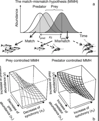
Fig. 1. The match-mismatch hypothesis (MMH) for the 2 models evaluated. (a) Cushing’s (1969, 1990) MMH based on time synchrony between predator (pred) and prey (prey)

(tpred− tprey= x2, the peaks time difference, Peaks T diff).

Arrows indicate opposite results for predators (solid arrows) and prey (dashed arrows). (b) MMHs with prey (left) and predator (right) control. In addition to the time component

(x2= Peaks T diff) prey abundance (x1, left, similar to Durant

et al. 2005) and predator abundance (x1, right) was added.

(c) The 2 statistical representations of the MMH, y = f (x1, x2).

f can be either a linear function or a nonparametric

Durant et al.: Match-mismatch hypothesis in predator-controlled systems 45

Predator-prey pairs

The pairs were chosen for their known relation-ships and for accessibility of data. The Narragansett Bay system is near the northern distribution limit of the ctenophore Mnemiopsis leidyi, which is not an invasive species in this region, in contrast to Euro-pean waters. The calanoid copepod Acartia tonsa is its major prey (Costello et al. 2006a, Costello et al. 2006b). In Skagerrak, the calanoid copepods

Calanus finmarchicus and C. helgolandicus

domi-nate the dry weight of the mesozooplankton and are known to graze on phytoplankton. C. helgo -landicus is the dominant large copepod in the

northern Skagerrak/North Sea. In the North Sea system, larval and juvenile Atlantic cod, Gadus

morhua, feed primarily on the calanoid copepods C. finmarchicus and Pseudocalanus spp. (Heath &

Lough 2007).

Data sources

In the Narragansett Bay estuary, data on the stand-ing stocks of Mnemiopsis leidyi and Acartia tonsa were collected at 2 locations in 2001−2003 and at 1 location in 2001−2004 (Costello et al. 2006a, Costello et al. 2006b). In the Skagerrak system, chlorophyll a (chl a) was sampled 3 times weekly during 1994− 2008 at the Flødevigen station (on the Norwegian Skagerrak coast), which is representative of the coastal waters of Northern Skagerrak (Dahl & Johan-nessen 1998), while the copepods Calanus

finmarchi-cus and C. helgolandifinmarchi-cus were sampled twice

monthly 1 nautical mile offshore from the station (for details of both sampling programs, see Johannessen et al. 2011). In the North Sea system, estimates of lar-val and juvenile cod abundances during 1988−2006, derived from virtual population analysis (see method in Lassen & Medley 2001), were obtained from ICES (www.ices.dk) and log-transformed. North Sea cope-pod data are from the Continuous Plankton Recorder Survey, an upper layer monitoring program that has operated on a monthly basis since 1946 (Reid et al. 2003).

Calculation of peaks time difference

The time coordinate of the centre of gravity was estimated for each variable and each year (Durant et al. 2005) in the 3 systems. The peaks time differ-ence (Peaks T diff), expressed in days, was then

calculated as the difference between the dates of maxi -mum predator and prey abundance (i.e. predator peak time − prey peak time or x2 = tpred − tprey in

Fig. 1a). When Peaks T diff = 0, the 2 peaks were synchronous, and when Peaks T diff = < 0, the prey appeared in the system after the predator (see also Fig. 2). Note that 0 indicates full synchrony but not necessarily a full match situation, because several days may be necessary to reach it — e.g. time is needed for a larval fish to exhaust its yolk sac (see Laurel et al. 2011). For the Skagerrak system, we calculated the Peaks T diff between the peak of

Calanus (separately for C. finmarchicus and C. hel-golandicus) and the first peak of chl a. Because it

was not possible to obtain exact dates for North Sea cod, we assumed that they spawned in March (Brander 1994) and that hatching occurred a month later (Laurel et al. 2011).

Fig. 2. Calculation of the peaks time difference (Peaks T diff tpred– tprey) between predator and prey. (a) 2 situ ations

of prey phenology related to a predator phenology. Red: a case when prey appear before predators (Peaks T diff > 0). Blue: a case when prey appear after predators (Peaks T diff < 0). (b) Changes in Peaks T diff for a prey-con-trolled model. When the 2 peaks are synchronous (Peaks T diff = 0) the predator recruitment (‘Success’ in the plot)

Predator-prey models

We examined 2 statistical representations of the predator-prey relationship (Fig. 1c) following the general structure Yt= α + si(Xt) + εt, where s is a

non-parametric smoothing function specifying the effect of the covariates Xion the dependent variable Y in

year t, α is the intercept, and ε is a stochastic noise term. In the generalized additive model (GAM) for-mulation (see below) X can be either x1, x2 or an

interaction term (x1,x2). The interaction between x1

and x2defines a space where x1cannot affect Y

with-out x2and the converse.

The controlled model is the bottom-up, prey-controlled MMH where Y = predator recruitment,

x1= prey abundance, and x2= Peaks T diff.

The predator-controlled model is the top-down, predator-controlled MMH where Y = prey recruit-ment, x1 = predator abundance, and x2 = Peaks T

diff. A. tonsa (ind. m −3 ) 100 150 200 250 300 350 35 135 M. leidyi conc. (ind. m −3 ) a 0 100 200 300 Chl a (µg l −1 ) Chl a (µg l −1 ) b C. finnmarchicus (ind. m −2 ) 0 5 4 3 1 2 0 25 30 20 15 5 10 0 1000 600 200 0 1500 1000 500 0 3.0 1.0 2.0 0.0 1 –1 0 –2 3.0 1.0 2.0 0.0 100 200 300

Day of the year

Day of the year

Day of the year

c C. helgolandicus (ind. m −3 ) 2 4 6 8 10 12 Months Copepod abundance index d

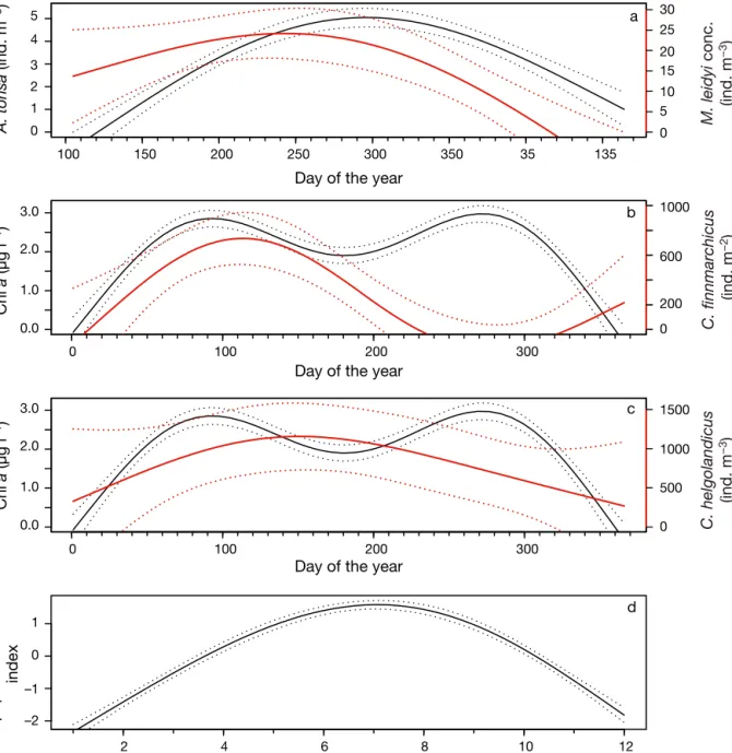
Fig. 3. Phenologies of the 3 systems. Solid lines: averages; dotted lines: SD. Red lines: prey; black lines: predators. (a) Narra-gansett Bay system, (b) and (c) Skagerrak system, (d) North Sea system (the North Sea cod eggs are assumed to hatch in April)

Durant et al.: Match-mismatch hypothesis in predator-controlled systems

Time series of predator abundance, prey abun-dance and the Peaks T diff between predator and prey (as individual species or species groups) were used to test both models in the 3 study systems.

Model testing

We tested the 2 models (prey-controlled and pred-ator-controlled) using a GAM (Wood & Augustin 2002, R Development Core Team 2010), as imple-mented in the mgcv library of R 2.11.1, correcting for overdispersion. The model selection was based on minimization of the generalized cross validation (GCV) score, and a measure of the model predictive squared error, the adjusted R2_{. Generalized cross}

validation is a proxy for the model’s out-of-sample predictive performance, analogous to the Akaike’s Information Criterion. This is the model selection pro cedure that is most appropriate for GAM analysis approaches (Wood & Augustin 2002, Wood 2011). The GAM procedure automatically chooses the degrees of freedom of the smoothing function s (i.e. the degree of linearity of the curve) based on the GCV score. However, to avoid spurious and ecolog-ically implausible relationships, we constrained the model to be at maximum a quadratic relationship. There was no temporal autocorrelation (using auto-correlation function ACF) in the residuals of the models.

The Narragansett Bay system

The abundance of Acartia tonsa and Mnemiopsis

leidyi (number of individuals m−3_{) was expressed in}

the models as the annual maximum value observed. A factor variable (Spot) was added to account for the potential effect of the 3 locations where the data were collected (i.e. Yt= α + s(Xt) + Spott+ εt).

The Skagerrak system

There are 2 chl a blooms per year in the bay (Fig. 3b,c): the first is dominated by diatoms and the second by dinoflagellates. Here we consider only the spring bloom occurring between January and July (days of the year between 0 and 180) because it occurs closer to the peaks of both Calanus species. Because the abundance data for C. finmarchicus and

C. helgolandicus exhibited a number of brief peaks

during its season, we used the average of the 5

high-est abundance values to minimize this variability in the models.

The North Sea system

For the prey-controlled model, recruitment was taken as the number of 1-year-old cod in the following year (CodRecr); for the predator-controlled model, recruitment was the sum of 1- and 2-year-old cod (CodAbun). One- to 2-year-old cod correspond to the age classes that prey on copepods, while the older cod feed on other species such as small fish and adult decapods. Both CodRecr and CodAbun were log-transformed. The plankton index of Beaugrand et al. (2003) was used to describe larval cod survival. This index is the first principal component calculated from a principal component analysis performed on long-term monthly abundance of Calanus finmarchicus, C.

helgolandicus, Pseudocalanus spp., euphausiids, total

biomass of calanoids and mean size of calanoid cope-pods between March and September. For the preda-tor-controlled model, we used the maximum plankton index value recorded between March and September (CopeIndMax) as an index of copepod abundance to estimate the annual copepod maximum. For the prey-controlled model, the annual average of the plankton index (CopeIndAv, cod consuming copepods through-out the entire annual cycle) was used.

RESULTS

The Narragansett Bay system

Prey-controlled model

The abundance of ctenophore Mnemiopsis leidyi was affected by the time between the ctenophore maximum and maxima of Acartia tonsa (Fig. 4a, Table 1). However, this model is suspicious because the quadratic shape is due to only 2 data points (Fig. 4a). This model was also significant when the abundance of A. tonsa was included in the analysis.

Predator-controlled model

The abundance of Acartia tonsa was positively affected by an increased time difference between the peaks of the ctenophore and A. tonsa (Fig. 4b, Table 1). The model was not significantly improved by including the abundance of the ctenophore.

● ● ● ● ● ● ● ● −80 −60 −40 −20 0 20 40 −80 −60 −40 −20 0 20 140 120 100 80 60 20 15 10 5 20 15 10 5 5 4 3 2 1 40 80 60 −40 −20 0 1400 1000 600 200 150 100 50 20 15 10 14 13 12 5 0 0 20 40 80 100 120 60 20 40 0 20 40 60 80 100 120 −40 −20 0 20 40 −4 −6 −2 0 2 4 12.0 12.5 13.0 13.5 14.0 14.5 15.0

Peaks T diff (d) Peaks T diff (d)

Peaks T diff (d) Peaks T diff (d)

Peaks T diff (d) Peaks T diff (d)

M. leidyi (ind. m −3 ) Prey-controlled models a ● ● ● ● ● ● ● ● A. tonsa (ind. m −3 ) Predator-controlled models b ● ● ● ● ● ● ● ● ● ● ● ● ● ● ● C. finmarchicus (10 3 ind. m −2 ) c ● ● ● ● ● ● ● ● ● ● ● ● ● ● d ● ● ● ● ● ● ● ● ● ● ● ● ● ● C. helgolandicus (10 3 ind. m −2 ) e ● ● ● ● ● ● ● ● ● ● ● ● ● ● ● Chl a (µg l −1 ) C hl a (µg l −1 ) f ● ● ● ● ● ● ● ● ● ● ● ● ● ● ● ● ● ● ● ● ● ● ● ● ● ● ● ● ● ● ● ● ● ● ● ● ● ● ● ● ● ● ● ● CopeIndAv CodRecr g ● ● ● ● ● ● ● ● ● ● ● ● ● ● ● ● ● ● ● ● ● ● ● ● ● ● ● ● ● ● ● ● ● ● ● ● ● ● ● ● ● ● ● ● CodAbun CopeIndMax h

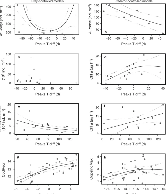
Fig. 4. Results from generalized additive models (GAMs) of the 4 prey/predator pairs. (a, b) Narragansett Bay, (c–f) Skagerrak, (g, h) the North Sea. Plots with a bold outline correspond to the most significant fit of the GAM models. For all peaks time difference (Peaks T diff) axes, 0 indicates full synchrony and a high absolute value indicates high asynchrony (see Fig. 2 and ‘Materials and methods’). (a) Ctenophore/copepodite pair where y-axis is Mnemiopsis leidyi abundance and x-axis is Peaks T diff with copepod prey. (b) Copepod/ctenophore pair where y-axis is Acartia tonsa abundance. (c) Copepod/chl a pair where

y-axis is Calanus finmarchicus abundance and x-axis is Peaks T diff with the first bloom of chl a. (d) Chl a/copepod pair where y-axis is chl a concentration of the first chl a bloom. (e) Copepod/chl a pair where y-axis is C. helgolandicus abundance

and x-axis is Peaks T diff with the first bloom of chl a. (f) Chl a/copepod pair where y-axis is chl a concentration of the second chl a bloom. (g) Cod/copepod pair where y-axis is log-transformed cod recruitment (CodRecr) and x-axis is the CopeIndAv. (h) Copepod/cod pair where y-axis is the CopeIndMax index and x-axis is log -transformed cod abundance (CodAbun). For (g) CopeIndAv: average maximum plankton index value and for (h) CopeIndMax: maximum plankton index value. Note that (e) and (f) present only the Peaks T diff effect of the most significant models; a complete figure would include a third axis

Durant et al.: Match-mismatch hypothesis in predator-controlled systems

The Skagerrak system

Prey-controlled models

No significant model explained the changes of

Calanus finmarchicus abundance (Table 1). The best

model selected by GCV was the null model (Fig. 4c).

The abundance of Calanus helgolandicus was explained by the interaction between Peaks T diff and the magnitude of the chl a bloom (Table 1). The increase of the time between the 2 peaks led to a lower abundance of C. helgolandicus (Fig. 4e) while the increase of chl a had a positive effect on the abundance of C. helgolandicus.

49

System Yt Explanatory variables, Xt n Fig. 4 p Adjusted R2 GCV

Narragansett Prey-controlled

Bay Mnemiopsis leidyit Peaks T difft −,+ 8 a 0.024 0.87 127

(Acartia tonsat, Peaks T difft) 8 0.063 0.94 112

A. tonsat + 8 0.401 0.35 574

NULL 8 0.04 518

Predator-controlled A. tonsat Peaks T difft − 8 b 0.020 0.91 2.5 M. leidyit + 8 0.472 0.28 15.6 (M. leidyit, Peaks T difft) 8 0.672 0.18 24.1 NULL 8 0.15 13.0 Skagerrak Prey-controlled Calanus finmarchicust Peaks T difft − 15 0.522 0 33937

Chl at +/− 15 0.377 0 34481

(Chl at,Peaks T difft) 15 0.660 0 40688

NULL 15 c 0 32462

Predator-controlled Chl at Peaks T difft + 14 d 0.036 0.38 1.224 (C. finmarchicust,Peaks T difft) 14 0.145 0.19 1.623 C. finmarchicust + 14 0.761 0.08 2.084 NULL 14 0 1.790 Skagerrak Prey-controlled Calanus helgolandicust (Chl at, Peaks T difft) 14 e 0.008 0.63 1700

Peaks T diff_t − 14 0.070 0.14 2518

Chl at + 14 0.098 0.13 2666

NULL 14 0 2869 Predator-controlled

Chl at (C. helgolandicust,Peaks T difft) 15 f 0.109 0.25 25.64

Peaks T difft + 15 0.400 0.02 27.40

C. helgolandicust +/− 15 0.666 0.01 30.03

NULL 15 0 30.27 North Sea Prey-controlled

CodRecrt+1 CopeIndAvt + 45 g < 0.001 0.55 0.031

(CopeIndAvt,Peaks T difft) 45 < 0.001 0.54 0.032

Peaks T difft + 45 0.006 0.15 0.059

NULL 45 0 0.067 Predator-controlled

CopeIndMaxt CodAbunt + 44 h 0.015 0.15 0.393

(CodAbunt,Peaks T difft) 44 0.037 0.09 0.424

Peaks T difft + 45 0.205 0.01 0.461

NULL 45 0 0.457 Table 1. Results of the generalized additive models of the relationship between predator-prey abundances and peaks time dif-ference. Models are written Yt= α + s (Xt) + εt, with s, a nonparametric smoothing function specifying the effect of the

covari-ates X on the dependent variable Y for year t; α, intercept; and ε, stochastic noise term. Xt= (Acartia tonsat, Peaks T difft) cor

-responds to an interaction term. For the models without interaction (e.g. Xt = Peaks T difft), the general sense of the

relationship is indicated with + or − (where both symbols are used, this indicates a quadratic relationship) as is the p-value and the generalized cross validation (GCV) score. Significant p-values are shown in bold. The plot of Fig. 4 is given for the selected models. Peaks T diff: peaks time difference; chl a: chlorophyll a concentration; CodRecr: ln(cod recruitment); CopeIndAv: average maximum plankton index value; CopeIndMax: maximum plankton index value; CodAbun: ln(cod abundance)

Predator-controlled model

The concentration of chl a was affected by the interaction between Peaks T diff and maximum abundance of Calanus finmarchicus (Table 1): greater abundance of C. finmarchicus led to a lower chl a bloom. The Peaks T diff spanned between −40 and + 40 d. The chl a bloom was smallest when C.

fin-marchicus reached maximum abundance 40 d before

the chl a maximum (Fig. 4d).

When considering Calanus helgolandicus, no sig-nificant model explained chl a changes (Table 1). The best model selected by GCV used the interaction between Peaks T diff and the maximum abundance of C. helgolandicus, with a positive effect of an increase in Peaks T diff (Fig. 4f).

The North Sea system

Prey-controlled model

Cod recruitment (CodRecr) was influenced posi-tively by the indicator CopeIndAv (Fig. 4g, Table 1). The model was not significantly improved by adding the time component. The Peaks T diff alone affected cod recruitment positively, but not strongly.

Predator-controlled model

Copepod abundance (CopeIndMax) was affected positively by cod abundance (CodAbun) (Fig. 4h, Table 1). The model was not improved significantly by adding the Peaks T diff. The Peaks T diff alone did not affect copepod abundance significantly.

DISCUSSION

The MMH assumes that variations in marine fish year-class strength are rooted in the fixity of the fish spawning time in relation to variable zooplank-ton abundance, i.e. predator (larval fish) abundance depends on prey abundance. Thus, the MMH makes sense only if prey biomass controls predator biomass, a relationship controlled from the bottom-up. In predator-controlled, top-down trophic rela-tionships, changes in prey biomass should not sta-tistically affect the predator biomass. Hence, the MMH cannot be applied to a predator-controlled trophic relationship without considering the more general version of the hypothesis, that the

abun-dance of individual species depends on synchrony with adjacent trophic levels, including synchrony with prey increases (prey-controlled MMH) as well as synchrony with predator decreases (predator-controlled MMH).

In this study, we statistically tested whether the MMH can be applied in different marine systems characterized by bottom-up or top-down control, or both. In the Narragansett Bay estuary, where it is well documented that the abundance of Acartia

tonsa is controlled by Mnemiopsis leidyi (Deason &

Smayda 1982, Sullivan et al. 2007, Sullivan et al. 2008), we found that the predator-controlled MMH model (Table 1) explained changes in prey abun-dance. The significance of the predator-controlled model was expected, because M. leidyi is widely associated with top-down control of plankton dynam-ics in systems where it is native as well as invasive (Purcell et al. 2001, Costello et al. 2006a, Condon & Steinberg 2008, Kideys et al. 2008). In a sense, our results illustrate the control of population dynamics by predation with the addition of a time component to the analysis (Bollens et al. 1992). The prey -controlled model was also statistically significant, but presents 2 challenges. First, the relationship shows a U shape, which would be expected for a predator-controlled relationship; however, the U shape is due to only 2 data points associated with a very wide con-fidence interval, rendering the model unrealistic (Fig. 4a). Second, the model shows an increase in ctenophore abundance associated with an increase in the time separating the 2 abundance maxima (i.e. the peak of M. leidyi occurring earlier and earlier than the peak of A. tonsa). Such a pattern is expected for a predator-controlled relationship, i.e. A. tonsa preying on M. leidyi, which is not the case. This result may thus be an artefact of using the prey -controlled model in a case where a strong predator-controlled model applies.

In the Skagerrak system, the chl a bloom depended on the level of synchrony between peaks of abun-dance of chl a and Calanus finmarchicus (predator-controlled model) (Fig. 4d). This result suggests that

C. finmarchicus limited the phytoplankton bloom in a

typical top-down control relationship. In contrast, the abundance of C. helgo landicus was higher when its peak of abundance was synchronous with the chl a bloom (prey-controlled model) (Fig. 4e), indicating a bottom-up controlled relationship. Thus, the 2 cope-pod species appeared to have very different relation-ships to their prey during the spring bloom, which in turn may have a large effect on the entire ecosystem (Beaugrand et al. 2003, Johannessen et al. 2011)

Durant et al.: Match-mismatch hypothesis in predator-controlled systems

For North Sea cod larvae and juveniles, which are well documented to be prey-controlled (Beaugrand et al. 2003, Durant et al. 2005, Olsen et al. 2011), we found that the prey-controlled model (Table 1, Fig. 4g) explained the change in abundance. The time difference between the peaks of abundance had a significant but minor effect, most likely because alternative prey may be available to cod over the entire annual cycle. The predator controlled model was significant, but the effect of cod abundance on plankton was opposite to what was expected (i.e. a positive effect) (Fig. 4h). This positive effect of cod may be explained by the negative effect of cod pre-dation on another copepod grazer, such as the her-ring Clupea harengus. However, the second best, and also significant, model selected by GCV (Table 1) indicated that the highest copepod abundances were associated with both high cod abundances and high time difference between the peaks of abundance. In other words, cod had a stronger positive effect on copepods when the copepod peak occurred late in the season. This result may thus be an artefact of using the predator controlled model in a case where a strong prey controlled model applies.

The results for Narragansett Bay and the North Sea systems illustrate the limitation of our analyses: when a strong relationship exists between predator and prey, both formulations (i.e. prey = f[predator] and predator = f[prey]) are significant when evaluated using the same data. Consequently, it is difficult to determine whether the predator or the prey controls the interaction without knowing the structure and function of the entire system. In the North Sea sys-tem, the discrepancy between the synchrony effect and abundance prompts us to select the prey -controlled model as most appropriate. In the case of Narragansett Bay system, we based our conclusions on the observation that Mnemiopsis leidyi can nearly extirpate Acartia tonsa from the bay when it colo-nizes the system during periods of increased temper-atures (Costello et al. 2006a,b, Sullivan et al. 2007).

There is now evidence that climate change can lead to differential changes in the occurrence of predators and their prey in marine pelagic systems (Platt et al. 2003), with the potential to increase phe-nological mismatch (Cury et al. 2008). In some cases this may modify the structure of the system, e.g. by changing the dominant species. For example, Acartia

tonsa was historically the dominant secondary

pro-ducer in the Narragansett Bay system (e.g. Hulsizer 1976) because its period of highest production in July occurred prior to the seasonal appearance of

Mne-miopsis leidyi in late summer (Durbin & Durbin

1981). Recent warmer spring temperatures have advanced the seasonal appearance of M. leidyi in the bay, but not that of A. tonsa (Costello et al. 2006a), leading to a temporal match and the copepod’s near extirpation from the system.

Both our theoretical arguments and empirical analyses extend discussion of the match-mismatch hypothesis and of predator control of lower trophic levels by upper trophic levels. An advantage of our approach is that the match-mismatch models can be applied to evaluate the relative strength of predator or prey control in a predator-prey pair. However, doing so requires relatively long-term series data of good quality. The models also have the ability to sep-arate within-season temporal shifts of trophic syn-chrony from an annual component linked to total predator/ prey abundance. In our view, this improves our ability to predict the negative effects of predation in a changing environment.

Acknowledgements. The Norwegian Research Council

sup-ported this research through the MICO project. The Norwe-gian Pollution Control Authority funded the Skagerrak data collection (the Coastal Water Monitoring Program). The US National Science Foundation funded the Narragansett Bay study. We thank 2 anonymous referees for their comments on our manuscript.

LITERATURE CITED

Beaugrand G, Brander KM, Lindley JA, Souissi S, Reid PR (2003) Plankton effect on cod recruitment in the North Sea. Nature 426: 661−664

Bollens SM, Frost BW, Schwaninger HR, Davis CS, Way KJ, Landsteiner MC (1992) Seasonal plankton cycles in a temperate fjord and comments on the match-mismatch hypothesis. J Plankton Res 14: 1279−1305

Brander KM (1994) The location and timing of cod spawning around the British isles. ICES J Mar Sci 51: 71−89 Condon RH, Steinberg DK (2008) Development, biological

regulation, and fate of ctenophore blooms in the York River estuary, Chesapeake Bay. Mar Ecol Prog Ser 369: 153−168

Costello JH, Sullivan BK, Gifford DJ (2006a) A physical-bio-logical interaction underlying variable phenophysical-bio-logical responses to climate change by coastal zooplankton. J Plankton Res 28: 1099−1105

Costello JH, Sullivan BK, Gifford DJ, Van Keuren D, Sulli-van LJ (2006b) Seasonal refugia, shoreward thermal amplification, and metapopulation dynamics of the ctenophore Mnemiopsis leidyi in Narragansett Bay, Rhode Island. Limnol Oceanogr 51: 1819−1831

Cury PM, Shin YJ, Planque B, Durant JM and others (2008) Ecosystem oceanography for global change in fisheries. Trends Ecol Evol 23: 338−346

Cushing DH (1969) The regularity of the spawning season of some fishes. J Cons Int Explor Mer 33: 81−92

Cushing DH (1990) Plankton production and year-class 51

➤

➤

➤

➤

➤

➤

➤

➤

➤

➤

strength in fish populations: an update of the match/mis-match hypothesis. Adv Mar Biol 26: 249−293

Dahl E, Johannessen T (1998) Temporal and spatial variabil-ity of phytoplankton and chlorophyll a: lessons from the south coast of Norway and the Skagerrak. ICES J Mar Sci 55: 680−687

Deason EE, Smayda TJ (1982) Experimental evaluation of herbivory in the ctenophore Mnemiopsis leidyi relevant to ctenophore-zooplankton-phytoplankton interactions in Narragansett Bay, Rhode Island, USA. J Plankton Res 4: 219−236

Durant JM, Hjermann DØ, Anker-Nilssen T, Beaugrand G, Mysterud A, Pettorelli N, Stenseth NC (2005) Timing and abundance as key mechanisms affecting trophic interactions in variable environments. Ecol Lett 8: 952−958

Durant JM, Hjermann DØ, Ottersen G, Stenseth NC (2007) Climate and the match or mismatch between predator requirements and resource availability. Clim Res 33: 271−283

Durbin AG, Durbin EG (1981) Standing stock and estimated production rates of phytoplankton and zooplankton in Narragansett Bay, Rhode Island. Estuaries 4: 24−41 Heath MR, Lough RG (2007) A synthesis of large-scale

pat-terns in the planktonic prey of larval and juvenile cod

(Gadus morhua). Fish Oceanogr 16: 169−185

Hulsizer EE (1976) Zooplankton of lower Narragansett Bay, 1972−1973. Chesap Sci 17: 260−270

Johannessen T, Dahl E, Falkenhaug T, Naustvoll LJ (2011) Concurrent recruitment failure in gadoids and changes in the plankton community along the Norwegian Skager-rak coast after 2002. ICES J Mar Sci 69: 795−801 Kideys AE, Roohi A, Eker-Develi E, Mélin F, Beare D (2008)

Increased chlorophyll levels in the southern Caspian Sea following an invasion of jellyfish. Res Lett Ecol 2008: Article ID 185642

Lassen H, Medley P (2001) Virtual population analysis — a practical manual for stock assessment. FAO Fish Tech Pap 400. FAO, Rome

Laurel BJ, Hurst TP, Ciannelli L (2011) An experimental examination of temperature interactions in the

match-mismatch hypothesis for Pacific cod larvae. Can J Fish Aquat Sci 68: 51−61

Olsen EM, Ottersen G, Llope M, Chan KS, Beaugrand G, Stenseth NC (2011) Spawning stock and recruitment in North Sea cod shaped by food and climate. Proc R Soc Lond B Biol Sci 278: 504−510

Platt T, Fuentes-Yaco C, Frank KT (2003) Spring algal bloom and larval fish survival. Nature 423: 398−399

Purcell JE, Shiganova TA, Decker MB, Houde ED (2001) The ctenophore Mnemiopsis in native and exotic habi-tats: U.S. estuaries versus the Black Sea basin. Hydrobi-ologia 451: 145−176

R Development Core Team (2010) R: A language and envi-ronment for statistical computing. R Foundation for Statis-tical Computing, Vienna, available at www. R-project.org Reid PC, Colebrook JM, Matthews JBL, Aiken J, Continu-ous Plankton Recorder Team (2003) The continuContinu-ous plankton recorder: concepts and history, from plankton indicator to undulating recorders. Prog Oceanogr 58: 117−173

Sinclair ARE, Krebs CJ (2002) Complex numerical responses to top-down and bottom-up processes in vertebrate pop-ulations. Philos Trans R Soc B 357: 1221−1231

Sullivan BK, Costello JH, Van Keuren D (2007) Seasonality of the copepods Acartia hudsonica and Acartia tonsa in Narragansett Bay, RI, USA during a period of climate change. Estuar Coast Shelf Sci 73: 259−267

Sullivan BK, Gifford DJ, Costello JH, Graff JR (2008) Narragansett Bay ctenophore-zooplankton-phytoplank-ton dy namics in a changing climate. In: Desbonnet A, Costa-Pierce B (eds) Science for ecosystem-based management: Narragansett Bay in the 21st century. Springer Series on Environmental Management, Springer, New York, NY, p 485–490

Wood SN (2011) Fast stable restricted maximum likelihood and marginal likelihood estimation of semiparametric generalized linear models. J R Stat Soc B 73: 3−36 Wood SN, Augustin NH (2002) GAMs with integrated model

selection using penalized regression splines and applica-tions to environmental modelling. Ecol Model 157: 157−177

Editorial responsibility: Kenneth Sherman, Narragansett, Rhode Island, USA

Submitted: April 16, 2012; Accepted: October 3, 2012 Proofs received from author(s): January 18, 2013

➤

➤

➤

➤

➤

➤

➤

➤

➤

➤

➤

➤

➤

➤

➤

➤

➤

➤

➤

➤

➤