HAL Id: hal-00304780
https://hal.archives-ouvertes.fr/hal-00304780
Submitted on 1 Jan 2003HAL is a multi-disciplinary open access archive for the deposit and dissemination of sci-entific research documents, whether they are pub-lished or not. The documents may come from teaching and research institutions in France or abroad, or from public or private research centers.
L’archive ouverte pluridisciplinaire HAL, est destinée au dépôt et à la diffusion de documents scientifiques de niveau recherche, publiés ou non, émanant des établissements d’enseignement et de recherche français ou étrangers, des laboratoires publics ou privés.
precipitation-runoff model for Norway
S. Beldring, K. Engeland, L. A. Roald, N. R. Sælthun, A. Voksø
To cite this version:
S. Beldring, K. Engeland, L. A. Roald, N. R. Sælthun, A. Voksø. Estimation of parameters in a distributed precipitation-runoff model for Norway. Hydrology and Earth System Sciences Discussions, European Geosciences Union, 2003, 7 (3), pp.304-316. �hal-00304780�
Estimation of parameters in a distributed precipitation-runoff
model for Norway
Stein Beldring
1, Kolbjørn Engeland
1, Lars A. Roald
1, Nils Roar Sælthun
2and Astrid Voksø
11Norwegian Water Resources and Energy Directorate, P.O. Box 5091 Majorstua, 0301 Oslo, Norway 2Norwegian Institute for Water Research, P.O. Box 173 Kjelsås, 0411 Oslo, Norway
Email for corresponding author: [email protected]
Abstract
A distributed version of the HBV-model using 1 km2 grid cells and daily time step was used to simulate runoff from the entire land surface of
Norway for the period 1961-1990. The model was sensitive to changes in small scale properties of the land surface and the climatic input data, through explicit representation of differences between model elements, and by implicit consideration of sub-grid variations in moisture status. A geographically transferable set of model parameters was determined by a multi-criteria calibration strategy, which simultaneously minimised the residuals between model simulated and observed runoff from 141 Norwegian catchments located in areas with different runoff regimes and landscape characteristics. Model discretisation units with identical landscape classification were assigned similar parameter values. Model performance was evaluated by simulating discharge from 43 independent catchments. Finally, a river routing procedure using a kinematic wave approximation to open channel flow was introduced in the model, and discharges from three additional catchments were calculated and compared with observations. The model was used to produce a map of average annual runoff for Norway for the period 1961-1990.
Keywords: distributed model, multi-criteria calibration, global parameters, ungauged catchments
Introduction
Regional scale hydrological models, which describe the water balance of the land surface over spatial domains
ranging from approximately 104 km2 to entire continents,
are widely used in water resources assessments; e.g. quantifying flood hazards, sediment transport, hydroelectric potential, water availability for agriculture and the impacts of changes in land use or climate. These models are also input to terrestrial ecosystem models, and represent hydrological processes in regional and global scale atmospheric models (Vörösmarty et al., 1993). Irrespective of the purpose of regional scale hydrological modelling, there is a need to describe the variability of the relevant hydrological variables and fluxes at different spatial scales. Because the data required for calibration are available only at a limited number of sites, regional models must perform well under conditions of geographical transposability and non-stationarity as defined by Kleme (1986).
Hydrological models are often lumped spatially with calibrated effective parameters which are assumed to take into account all of the local heterogeneity of land surface characteristics, meteorological variables and hydrological processes for large areas. In view of the natural variability of the landscape and the non-linearity of the processes involved, this approach is inappropriate for generalising information about hydrological behaviour from gauged catchments to large regions. One solution to this problem is to describe the distribution of properties within the model elements. Ewen et al. (1997) accounted for the effects of sub-grid variations in moisture status and landscape properties by considering the fractions of model grid cells associated with shallow and deep water tables. Alternatively, Becker and Braun (1999) recommended that hydrological models should apply a process-adequate areal discretisation scheme, where individual model elements act as hydrological response units, i.e. patches in the landscape
mosaic having a common climate, land use and pedological, topological and geological conditions controlling their hydrological process dynamics (Flügel, 1995). Motovilov
et al. (1999) addressed the problem of aggregating the
dynamic behaviour of land surface hydrological processes to larger scales in the presence of natural heterogeneity; the landscape was divided into elements large enough to include the different types of hydrological response units in each land use class and the contributions from the individual elements were then integrated. In the general case, this type of subdivision will have to consider variations in geology, soils, topography, vegetation and other landscape characteristics which control the water balance of catchments (Bork and Rohdenburg, 1986; Benosky and Merry, 1995). A physically realistic framework for regional scale modelling of land surface hydrology is, therefore, provided by models which integrate the contributions from several small scale elements. The regional models must also account for the water balance of ungauged areas where no data are available for model calibration. Model parameters must therefore be estimated using information about land surface properties and hydrological data from other parts of the region of interest (Gottschalk et al., 2001). This implies repeated application of the hydrological model everywhere within a region using a geographically transferrable set of parameters (Kleme, 1986). Dunn and Lilly (2001) followed this approach in an investigation of the relationship between a soil classification system and the parameter values of a spatially distributed hydrological model. Landscape elements which could be expected to have similar hydrological behaviour were parameterised in the same way and calibrated parameter sets were transferred from one discretisation unit to another.
The landscape of the Scandinavian countries is dominated by boreal forests and mountains, with distinct topographic features such as valleys, hills, ridges and plateaus shaped beneath great Pleistocene ice sheets. Exposed bedrock and shallow till deposits interspersed with isolated glaciofluvial deposits cover the land surface. Streams, lakes and bogs abound and glaciers occur frequently in western and northern parts. This mosaic of terrain elements creates a heterogeneous lower boundary to the atmosphere with highly differing thermal, roughness and radiative properties. Small scale phenomena influence the exchange processes between the land surface and the atmosphere and the lateral redistribution of water through subsurface and surface flows (Halldin et al., 1999). The objectives of the present study were: (i) to determine a globally applicable set of parameters for distributed hydrological modelling in this environment by including information about physical landscape characteristics in the parameterisation procedure, and (ii)
to model the dynamics of hydrological processes in gauged and ungauged catchments in Norway to produce a map of average annual runoff for the period 19611990. The effects of including a river routing procedure in the model was investigated for a mountainous area in eastern Norway.
Distributed hydrological model
The strategy is a bottom-up approach to construction of hydrological models as described by Kleme (1983), using a spatially distributed version of the HBV-model (Bergström, 1995). The model performs water balance calculations for square grid cell landscape elements characterised by their altitude and land use. Each grid cell may be divided into two land use zones with different vegetations, a lake area and a glacier area. The model is run with daily time step, using measurements of precipitation and air temperatures as input. It has components for accumulation, sub-grid scale distribution and ablation of snow, interception storage, sub-grid scale distribution of soil moisture storage, evapotranspiration, groundwater storage and runoff response, lake evaporation and glacier mass balance. The model considers the effects of seasonally varying vegetative characteristics on potential evaporation. The algorithms of the model were described by Bergström (1995) and Sælthun (1996). The model is spatially distributed because every model element has unique characteristics that determine its parameters, input data are distributed, water balance computations are performed separately for each model element and, finally, only those parts of the model structure that are necessary are used for each element. When water divides are determined, runoff from the individual model grid cells is sent to the respective catchment outlets without delay.
The routing of runoff through the river network is an important component of distributed hydrological models when considering time series of flows from large drainage basins (Naden, 1993). Based on work by Motovilov et al. (1999), a method for describing the hierarchy of the river network and a procedure for modelling flow in rivers and lakes were included in the distributed model. River flow is calculated by a kinematic wave approximation to the governing equations of open channel flow, while outflows from lakes are modelled using the equations for linear reservoirs based on inflows. With the routing procedure included, each discretisation unit of the model is assumed to drain into the nearest river segment or lake element in the river network hierarchy, i.e. no subsurface or overland flow takes place between the landscape elements. The river elements are located between the landscape elements and all have length equal to the size of the grid cells. The lake
elements, modelled as part of the river network hierarchy, cover complete grid cells, i.e. no other land use types may exist within them. A description of lakes is, therefore, included both in the river network hierarchy and as part of the landscape elements.
Multi-criteria calibration
The information in the precipitation-runoff relationship is usually insufficient to allow identification of unique values for the parameters of a hydrological model (Jakeman and Hornberger, 1993). This identifiability problem makes it difficult to determine one consistent, globally applicable parameter set from several individually calibrated catchments (Kuczera and Mroczkowski, 1998). However, use of runoff data from multiple catchments, or of both runoff and additional measurements such as groundwater levels during the calibration process, may enhance model performance and improve the consistency and stability of parameter estimates (Sorooshian and Gupta, 1995; Beldring, 2002a). Motovilov et al. (1999) and Engeland et al. (2001) demonstrated that calibration using runoff from several catchments within a region reduces the uncertainty in the values of the parameters of a distributed hydrological model, provided that model parameters are conditioned on land surface properties. When these multi-criteria calibration strategies are applied, simultaneously objective measures of several aspects of model performance have to be considered (Gupta et al., 1998; Yapo et al., 1998).
In a distributed hydrological model, the approach to finding a globally applicable set of parameters must include information on physical landscape characteristics in the parameterisation procedure and in the model calibration strategy (Gottschalk et al., 2001). The model discretisation units should represent the significant and systematic variations in the properties of the land surface and representative (typical) parameter values must be applied for different classes of soil and vegetation types, lakes and glaciers (Refsgaard, 1997). The globally applicable parameter set is found by calibrating the model with the restriction that the same parameter values are used for all computational elements of the model in the same class of land surface properties (Madsen, 2003). This calibration procedure rests on the hypothesis that model elements with identical landscape characteristics have similar hydrological behaviour, and should consequently be assigned the same parameter values. The model is calibrated using available information on climate and on hydrological processes from all gauged catchments with reliable observations and parameter values are transferred to other catchments based on the classification of landscape characteristics. Global
parameter sets may be used with good results in distributed hydrological models for large regions, provided realistic descriptions of hydrological processes and landscape characteristics are applied (e.g. Motovilov et al., 1999).
Several automatic calibration procedures, which use an optimisation algorithm to find those values of model parameters that minimize or maximize, as appropriate, an objective function or statistic of the residuals between model simulated output and observed catchment output, have been developed (e.g. Yapo et al., 1998). The nonlinear parameter estimation method PEST (Doherty et al., 1998) was used to adjust the parameters of a model within individually specified lower and upper bounds until the sum of squares of residuals between selected model outputs and a complementary set of observed data are minimal. A multi-criteria calibration strategy was applied, where the residuals between model-simulated and observed monthly runoff from several catchments located in areas with different runoff regimes and landscape characteristics were considered simultaneously.
Although the distributed HBV-model operates on a daily time step and has procedures for river and lake routing, monthly runoff data were used during calibration, as the use of daily values would have required a description of the river network in all the larger catchments and this was not available. Furthermore, backwater effects due to ice jamming occur in the winter in many regions in Norway. The procedures for ice reduction are not as reliable as could be desired, and monthly data which are corrected on the basis of total runoff volumes are usually more reliable than daily values which must consider individual runoff events.
Process parameterisation
As a distributed model potentially includes a huge number of parameters, rigorous parameterisation is crucial for proper model calibration (Madsen, 2003), so the recommendations of Gottschalk et al. (2001) were adopted; they argued that effective parameters should take into account all of the local scale heterogeneity of soil and vegetation type, topographic position, surface roughness, water stress and meteorological variables that influence the landscape scale integrated fluxes. With a few exceptions, inputs and state variables are interpreted as averages over the fundamental model units.
An important issue in connection with process parameterisation is identification of the appropriate scale of the computational units. Reggiani et al. (2000) suggested that the discretisation units of a distributed hydrological model should contain all basic hydrological processes, including saturated and unsaturated subsurface zones,
saturated and concentrated overland flow zones, and a river channel. No mass is transferred laterally across the prismatic surface delimiting these units. Hydrological processes with characteristic length scales longer than the computational element size are represented explicitly by element to element variations, whereas processes with length scales shorter than the element size are represented implicitly. The same parameterisation procedure can be used for all computational elements which contain a similar sample of geology, soils, topography, vegetation and other relevant characteristics which determine runoff and evapotranspiration fluxes. For each of these sub-regions, all associated variables and properties are lumped spatially and can vary only with time. The permanent river network including streams and lakes lies within 1 km of almost every point in the Norwegian landscape. The parameterisation procedure, therefore, attempts to link landscape characteristics and conceptual type process descriptions for 1 km2 grid cells, on the assumption that all lateral transfers of water at this spatial scale take place in the river network. Representative process descriptions and parameter values are applied for different land use classes, lakes and glaciers.
The parameter values assigned to the computational elements of the precipitation-runoff model should reflect the fact that hydrological processes are sensitive to spatial variations in soil properties (e.g. Merz and Plate, 1997) and vegetation (e.g. VanShaar et al., 2002). As the Norwegian landscape is dominated by shallow surface deposits overlying a relatively impermeable bedrock, the capacity for subsurface storage of water is small (Beldring, 2002b). Monthly runoff used during model calibration is, therefore, more sensitive to the intensity of evapotranspiration and the occurence of snow accumulation and ablation than to soil properties controlling temporary storage of water and runoff event hydrographs. However, the spatial variability in maximum soil moisture storage must be taken into account Areas with low capacity for soil water storage will be depleted faster and reduced evapotranspiration caused by moisture stress shows up earlier than in areas with high capacity for soil water storage (Zhu and Mackay, 2001).
Vegetative characteristics such as stand height and leaf area index influence the water balance at different time scales through their control on evapotranspiration, snow accumulation and snow melt (Matheussen et al., 2000). The following land use classes were therefore used to describe the properties of the 1 km2 landscape elements of the model: (i) areas above the tree line with extremely sparse vegetation, mostly lichens, mosses and grass; (ii) areas above the tree line with grass, heather, shrubs or dwarfed trees; (iii) areas below the tree line with sub-alpine forests; (iv) lowland areas with coniferous or deciduous forests; and (v) non-forested
areas below the tree line, the upper margin of the sub-alpine forest where trees become dwarfed or are absent. The model was run with specific parameters for each land use class controlling snow processes, interception storage, evapotranspiration processes and maximum soil moisture storage. This classification does not identify, as separate land use classes, bogs or agricultural areas. Bogs were classified according to the characteristics of the vegetation by which they were covered, while agricultural areas are of minor importance in Norway as they constitute less than 3% of the land surface; they were, therefore, included in the non-forested areas below the tree-line. Furthermore, all land use classes were assumed to have identical parameters for groundwater storage and runoff response, as information about the hydrological characteristics of soils was unavailable. Lake evaporation and glacier mass balance were controlled by parameters with the same values for all model elements. Evapotranspiration and runoff from lakes and glaciers were controlled by parameters with global values. The streamflow time series were subject to double mass analysis (Alexandersson, 1986) and Pettitt-test (Pettit, 1979) to ascertain their consistency and quality. Although discharge determined from stage measurements and rating curves for natural conditions has an inherent uncertainty, the streamflow data used in this study are considered the most reliable in Norway. The uncertainty is largest during winter conditions, when ice in river cross sections and at lake outlets invalidate the rating curves that have been established for ice-free conditions. Observed water levels must be corrected by comparison with nearby stations not affected by ice before the rating curves can be applied. Since streamflow is low during periods with air temperatures below the freezing point, this uncertainty has a negligible effect on the annual water balance.
Data
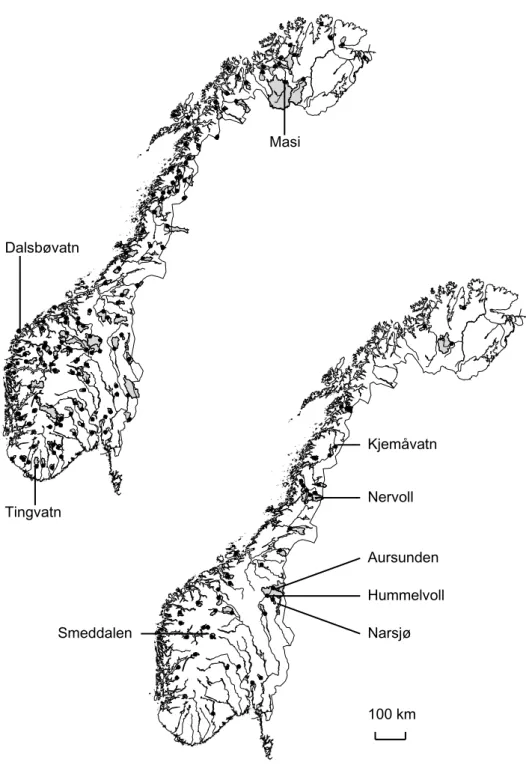
Data from the station network of the Hydrology Department, Norwegian Water Resources and Energy Directorate were used in calibration and validation of the model. Monthly runoffs from 141 catchments for the period 1 January 1968 to 31 December 1984 were used in model calibration; however, daily discharges from the same 141 catchments were also used to evaluate model performance. Monthly runoff and daily discharge from 43 independent catchments for the same period were used during model validation. The records for most of the validation catchments are incomplete, with up to three years data missing. All 184 catchments (Fig. 1) are situated between 58°24' and 70°55' N; they represent different landscape types, including mountains and alpine terrain, sub-alpine and boreal forests, non-forested
Fig. 1. Location of 141 catchments used to calibrate the distributed HBV-model (left) and 46 catchments used
in model validation (right). The names refer to the catchments shown in Figs. 35.
areas below the tree line, lakes, bogs and glaciers. Catchment
areas range from 4.3 to 5693 km2; the total area is 50 294
km2 and the catchments range from sea level to 2469 m.a.s.l. The climate varies from maritime to continental and several runoff regimes are classified according to seasonal variations of runoff (Gottschalk et al., 1979). At one extreme are catchments located in a mountain type regime with low flows in winter and dominant spring and summer high flows
caused by snowmelt; at the other extreme are catchments located in a coastal type regime with dominant autumn and winter high flows caused by rain, and summer low flows. Also, many catchments are in transitional regime types with varying degrees of dominance of spring snowmelt and autumn rain high flows.
To investigate the river routing procedure, daily discharges from three catchments in the upper River Glomma from 1
Tingvatn Dalsbøvatn Masi Smeddalen Nervoll Aursunden Hummelvoll Narsjø Kjemåvatn 100 km
September 1961 to 31 August 2000 were used. Two of these
catchments, Narsjø (119 km2) and Aursunden (835 km2) are
nested within the third, Hummelvoll (2469 km2). The climate in this area is continental and the runoff regime is of the mountain type. Monthly runoff data from the Narsjø catchment were also used during model calibration. Elevations within the Hummelvoll catchment range from 586 to 1595 m a.s.l, yet the landscape is relatively wide and open and the topography is gentle. Of the catchment area, 43% is covered by open mountain terrain without trees, 37% by sub-alpine and boreal forests (birch, spruce and pine), 11% by bogs, 7% by lakes and 2% by agricultural fields and meadows. The tree line within this area varies between 800 and 900 m a.s.l. The locations of all the catchments used in model calibration and validation are shown in Fig. 1. Daily mean values from 400 precipitation stations, corrected for wind and measurements losses and 93 temperature stations from the Norwegian Meteorological Institute were used as model inputs. Førland et al.,(1996) showed that the measured winter precipitation may be lower than 50% of the true amount in wind-exposed coastal and mountain areas, and the summer precipitation may also be underestimated substantially. Although the main errors in Nordic precipitation measurements are caused by aerodynamic effects near the rim of the gauges, significant errors may also be due to evaporation, wetting, drifting of snow, splashing in or out of the gauge, misreadings, leakage etc. The precipitation stations used in this study are classified in five exposure classes with fixed correction factors for rain, snow and mixed type precipitation. The precipitation data, accordingly, are given a simplified precipitation type classification. Precipitation and temperature values for the model grid cells are determined by inverse distance interpolation of observations from the three closest precipitation stations and the two closest temperature stations. Differences because of elevation are corrected by site specific precipitation altitude gradients and fixed temperature lapse rates for days with and without precipitation, respectively. During calibration, uncertainty in regard to the variations of precipitation with altitude in the mountainous terrain of Scandinavia (Johansson, 2000) was addressed by determining, for 29 locations in Norway, precipitation gradients with an exponential increase between 8% and 12% per 100 metres altitude; the values to be used for each grid cell were calculated by inverse distance interpolation using the three closest gradient points. These altitude gradients were reduced by 50% for elevations above 1200 m a.s.l., as drying out of ascending air occurs in high mountain areas due to orographically induced precipitation (Daly et al., 1994). The reduction of 50 % is chosen arbitrarily but the height of 1200 metres is not. This is the
approximate altitude of the coastal mountain ranges in W and N Norway and these mountains ranges release most of the precipitation associated with the eastward-migrating extra-tropical storm tracks that dominate the weather in Norway. The temperature lapse rates for days with and without precipitation were also determined by calibration but the same values were used for all grid cells. The simulations of discharge from the three catchments in the upper parts of the River Glomma used daily mean values from 15 precipitation stations and one temperature station as model input.
Digital map data from the Norwegian Mapping Authority were used to determine land use and elevation for each
model grid cell. Data sets resampled to a 1 km2 model grid
covering Norway were used: a mean elevation was based on a digital elevation model with horizontal resolution 100 m × 100 m and the proportions of grid area covered by forest, by lakes, and by glaciers. The land use proportions were based on vector data at a scale of 1:50 000 (lakes and glaciers) or 1:250 000. All other land use classes were classified as open land or mountain areas. To separate areas
above and below the tree line, a 1 km2 grid describing the
potential tree level was used. The potential tree level can be thought of as a continuous surface cutting through the landscape along the tree line. This information was determined by Strand (1998) by spatial interpolation (kriging) of tree level data from the Norwegian Mapping Authority. Data from a Norwegian vegetation atlas (Moen, 1998) were used to distinguish areas above the tree line with extremely sparse vegetation from areas above the tree line with grass, heather, shrubs or dwarfed trees, and to distinguish between areas below the tree line with sub-alpine forests and lowland areas with coniferous or deciduous forests. River network data in vector format (scale 1:50 000) were used for the routing model of the catchments in the upper parts of River Glomma.
Results
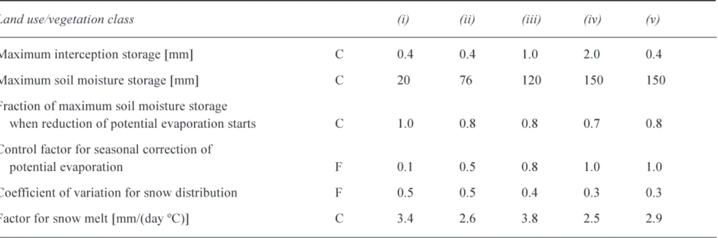
A total of 51 parameter values was optimised; 31 parameters describe the altitude gradients of precipitation and temperature, while four process parameters were assigned different values for each of the five land use classes. Each land use class was assigned different values for two additional process parameters but they were fixed, i.e. they were not determined by the calibration procedure. Table 1 presents the final values of the 30 parameters that were unique for each land use class; they determine the partitioning of rainfall or snowmelt into evapotranspiration and runoff, and control accumulation, sub-grid scale distribution and melting of snow for the different land use
classes. The remaining model parameters were fixed and equal for all land use classes. The parameter values were based on previous experience with the HBV-model in Sweden (Bergström, 1990) and Norway (Sælthun, 1996). Initial spin-up periods of three months were used to adjust the model before the calibration and validation procedures were started.
To have confidence in a hydrological model, its operational performance with regard to the relevant aspects of model behaviour must be validated (Sorooshian and Gupta, 1995). Model performance is usually evaluated by considering one or more objective statistics or functions of the residuals between model simulated output and observed catchment output. The objective functions used in this study were the Nash-Sutcliffe and bias statistics of the residuals, which are poorly correlated. The Nash-Sutcliffe efficiency criterion measures the fraction of the variance of the observations explained by the model, while bias (relative volume error) measures the tendency of the model-simulated values to be larger or smaller than their observed counterpart (Weglarczyk, 1998). The Nash-Sutcliffe efficiency criterion ranges from minus infinity to 1.0 with higher values indicating better agreement. It measures the fraction of the variance of observed values explained by the model:
(
)
(
)
2 1 2 1 1∑
∑
= = − − − = n t mean obs t n t sim t obs t q q q q NS(1)
where qtobs is observed catchment output at discrete
times t, qtsim is the corresponding model simulations,
qmean is the mean of the observed values, and n is the
Table 1. Values of model parameters which were unique for each land use/vegetation class
C = calibrated parameter, F = fixed parameter
The land use classes are: (i) areas above the tree line with extremely sparse vegetation, mostly lichens, mosses and grass; (ii) areas above the tree line with grass, heather, shrubs or dwarfed trees; (iii) areas below the tree line with subalpine forests; (iv) lowland areas with coniferous or deciduous forests; and (v) non-forested areas below the tree line
Land use/vegetation class (i) (ii) (iii) (iv) (v)
Maximum interception storage [mm] C 0.4 0.4 1.0 2.0 0.4
Maximum soil moisture storage [mm] C 20 76 120 150 150
Fraction of maximum soil moisture storage
when reduction of potential evaporation starts C 1.0 0.8 0.8 0.7 0.8 Control factor for seasonal correction of
potential evaporation F 0.1 0.5 0.8 1.0 1.0
Coefficient of variation for snow distribution F 0.5 0.5 0.4 0.3 0.3
Factor for snow melt [mm/(day ºC)] C 3.4 2.6 3.8 2.5 2.9
number of data points to be matched. Bias (relative volume error) measures the tendency of model simulated values to be larger or smaller than their observed counterpart:
(
)
∑
∑
= = − = n t obs t n t obs t sim t q q q BIAS 1 1(2)
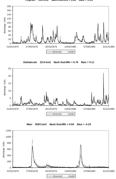
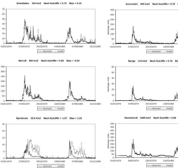
Although the Nash-Sutcliffe efficiency criterion is frequently used for evaluating the performance of hydrological models, it favours a good match between observed and modelled high flows, while sacrificing to some extent matching of below-mean flows (Houghton-Carr, 1999). It is for this reason that two different measures of model performance were considered.Figure 2 shows cumulative distribution functions of the values of Nash-Sutcliffe and bias statistics of monthly runoff for all catchments used during model calibration and validation and of daily discharge for 43 catchments used during model validation. Figure 3 shows observed and simulated daily discharge from three of the catchments used during calibration, while results for the three independent catchments used during validation are presented in Fig. 4.The result for the Kjemåvatn catchment shown in Fig. 4 is an example of unsatisfactory model simulations.
Results from simulating daily discharge from the catchments in the upper parts of River Glomma are shown in Fig. 5. The Aursunden catchment is regulated, model results were, therefore, compared to naturalised streamflow. Simulations for the Hummelvoll catchment were performed for the sub-catchment downstream of the Aursunden
Tingvatn 266 km2 Nash-Sutcliffe = 0.86 Bias = -0.03 0 20 40 60 80 100 120 140 160 180 01/01/1979 27/05/1979 20/10/1979 14/03/1980 07/08/1980 31/12/1980 di s c harge m 3 /s observed model
Dalsbøvatn 25.8 km2 Nash-Sutcliffe = 0.76 Bias = 0.11
0 5 10 15 20 25 01/01/1979 27/05/1979 20/10/1979 14/03/1980 07/08/1980 31/12/1980 di s c harge m 3 /s observed model
Masi 5693 km2 Nash-Sutcliffe = 0.84 Bias = -0.19
0 200 400 600 800 1000 1200 01/01/1979 27/05/1979 20/10/1979 14/03/1980 07/08/1980 31/12/1980 di s c harge m 3 /s observed model
Fig. 3. Observed and simulated daily streamflow from catchments
used in model calibration: Tingvatn (top), Dalsbøvatn (middle) and Masi (bottom). Only two years from the simulation period 1 January 1968 to 31 December 1984 are shown but the values of the Nash-Sutcliffe and bias statistics are based on the entire period.
catchment. In this case, observed discharge at the outlet of the Aursunden catchment was used as input to the river network. A snow pillow is located at Vauldalen (830 m a.s.l.) in the eastern part of the Aursunden catchment. Figure 6 shows that model values of snow water equivalent for the grid cell containing this snow pillow agree with observations for the period 1 September 1984 to 31 August 1997. Unfortunately, for some years the snow pillow was not in operation at the beginning of the winter.
The parameter set determined by the multi-criteria calibration strategy was used to produce a map of average annual runoff for the period 19611990 for Norway excluding the dependencies of Svalbard and Jan Mayen, an area of 323 758 km2. The model was run for all 1 km2 cells with a daily time step for the entire period with climate data
Calibration: Cumulative distribution functions of performance criteria for monthly runoff 0 0.2 0.4 0.6 0.8 1 -1.5 -1 -0.5 0 0.5 1 1.5 CDF
Bias (volume error) Nash-Sutcliffe efficiency
Validation: Cumulative distribution functions of performance criteria for monthly runoff 0 0.2 0.4 0.6 0.8 1 -1.5 -1 -0.5 0 0.5 1 1.5 CDF
Bias (volume error) Nash-Sutcliffe efficiency
Validation: Cumulative distribution functions of performance criteria for daily streamflow 0 0.2 0.4 0.6 0.8 1 -1.5 -1 -0.5 0 0.5 1 1.5 CDF
Bias (volume error) Nash-Sutcliffe efficiency
Fig. 2. Cumulative distribution functions of criteria of model
performance for monthly runoff for 141 catchments during calibration (top) and 43 catchments during validation (middle). Cumulative distribution functions of criteria of model performance for daily streamflow from 43 catchments during validation (bottom).
from the Norwegian Meteorological Institute as driving variables and an initial spin-up period of three months was used. The routine procedure was not applied. The ratios between observed average annual runoff and simulated average annual runoff were determined for 350 catchments for which the observations were considered reliable. If the catchments were nested, runoff from the inter-station sub-catchments were used. These ratios were applied as correction coefficients to be multiplied by the simulated annual runoff for each grid cell. An inverse distance interpolation procedure was performed to determine correction coefficients for catchments where the average annual runoff could not be determined from observations. A similar procedure was applied by Fekete et al. (1999) when calculating monthly runoff for the entire global land
Smeddalen 154 km2 Nash-Sutcliffe = 0.72 Bias = 0.10 0 10 20 30 40 50 60 70 01/01/1979 27/05/1979 20/10/1979 14/03/1980 07/08/1980 31/12/1980 di s c harge m 3 /s observed model
Nervoll 650 km2 Nash-Sutcliffe = 0.85 Bias = -0.04
0 50 100 150 200 250 300 350 01/01/1979 27/05/1979 20/10/1979 14/03/1980 07/08/1980 31/12/1980 di s c harge m 3 /s observed model
Kjemåvatn 35.6 km2 Nash-Sutcliffe = -1.57 Bias = 1.22
0 5 10 15 20 25 01/01/1979 27/05/1979 20/10/1979 14/03/1980 07/08/1980 31/12/1980 di s c harge m 3 /s observed model
Fig. 4. Observed and simulated daily streamflow from catchments
used in model validation: Smeddalen (top), Nervoll (middle) and Kjemåvatn (bottom). Only two years from the simulation period 1 January 1968 to 31 December 1984 are shown but the values of the Nash-Sutcliffe and bias statistics are based on the entire period.
Aursunden 835 km2 Nash-Sutcliffe = 0.76 Bias = -0.29
0 50 100 150 200 250 300 350 01/01/1979 27/05/1979 20/10/1979 14/03/1980 07/08/1980 31/12/1980 di s c harge m 3 /s observed model
Narsjø 119 km2 Nash-Sutcliffe = 0.78 Bias = -0.04
0 10 20 30 40 50 60 01/01/1979 27/05/1979 20/10/1979 14/03/1980 07/08/1980 31/12/1980 di s c harge m 3 /s observed model
Hummelvoll 2469 km2 Nash-Sutcliffe = 0.89 Bias = -0.06
0 50 100 150 200 250 300 350 400 450 500 01/01/1979 26/05/1979 19/10/1979 13/03/1980 06/08/1980 30/12/1980 di s c harge m 3 /s observed model
Fig. 5. Observed and simulated daily streamflow with procedures
for river and lake routing included for catchments: Aursunden (top), Narsjø (middle) and Hummelvoll (bottom). Only two years from the simulation period 1 September 1961 to 31 August 2000 are shown, but the values of the Nash-Sutcliffe and bias statistics are based on the entire period.
surface at 30-minute spatial resolution. Figure 7 shows the resulting runoff map, while Fig. 8 shows the correction coefficients which are an alternative way of expressing bias in the simulations.
Discussion
Table 1 presented parameter values that were unique for each land use/vegetation class. The values for maximum interception storage varies between the vegetation types in a reasonable manner. Maximum soil moisture storage is larger for lowland areas than for mountains; this is to be expected as the average thickness of surface deposits tends to decrease with altitude. Evapotranspiration is assumed to occur at the potential rate as long as soil moisture is above
a fraction of maximum soil moisture storage. Below this value, evapotranspiration decreases linearly to zero for soil moisture equal to zero. This parameter obtained the highest values for land use classes with shallow surface deposits where evapotranspiration must be expected to decrease below the potential rate at a higher degree of saturation than in areas with thick deposits. However, the value for non-forested areas below the tree line is possibly too high compared to lowland areas with forest. Potential evaporation is calculated as a linear function of temperature (above the freezing point) and is assumed to vary seasonally. A large value for the control factor for seasonal correction of potential evaporation leads to large variability within the year. The values of this parameter are large for lowland areas where biological activity is intense in summer and,
consequently, the seasonal variations in potential evaporation are large. For mountainous areas, the values for this parameter are small; potential evaporation varies less in these environments throughout the year. The model assumes a lognormal distribution of snow within each computational element. A value of the coefficient of variation equal to zero means that snow is evenly distributed, while the distribution becomes more skewed as the coefficient of variation increases. Wind exposed mountain areas generally have larger variability in snow cover than sheltered lowland areas and this is reflected by the parameter values. Snow melt is calculated by a temperature index approach where the melt factor determines the amount of snow melt when the temperature exceeds a threshold which was 0ºC for all land use classes. Although the temperature index method is a good approximation to more physically-based energy balance approaches, the melt factor must be expected to vary with atmospheric conditions, latitude, elevation, slope inclination and aspect, vegetative cover, and time of the year. It is not possible to draw any conclusions on the characteristics of the land use from the melt factor values determined by the calibration procedure.
The multi-criteria calibration strategy constrained model behaviour to runoff from catchments located in areas with different climate and land surface characteristics. The entire range of variations in hydrological processes in the Norwegian landscape were considered during this process, so the model was forced to simulate all possible combinations of natural conditions. The possibility of finding a robust parameter set increases if all operational modes of the model are activated during calibration (Sorooshian and Gupta, 1995), which may explain why the model performed reasonably well when daily values were considered. Approximately 75% of the monthly runoff series were simulated with values of the Nash-Sutcliffe efficiency criterion better than 0.5, while absolute values of the bias criterion were less than 0.3 for approximately 70% of the
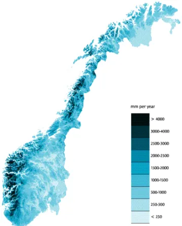
Fig. 7. Map of average annual runoff for Norway for the period
1961-1990. Spatial resolution 1 km2.
Fig. 8. Ratios between average annual runoff for Norway for the period 1961-1990 based on observations and the corresponding model generated values. Spatial resolution 1 km2.
Vauldalen Snow Water Equivalent
0 100 200 300 400 500 600 01/09/1984 01/09/1988 01/09/1992 01/09/1996 SW E mm observed model
Fig. 6. Observed and simulated daily snow water equivalent at
Vauldalen (830 m a.s.l.) in the eastern part of the Aursunden catchment for the period 1 September 1984 to 31 August 1997.
monthly series. The results deteriorated when daily values were considered; nevertheless approximately 60% of the daily discharge series obtained better values than the above mentioned thresholds, for both criteria. These results apply both during calibration and validation and indicate, strongly, that the parameterisation and calibration procedures determine parameter sets that may be used to predict runoff in ungauged catchments. Although model performance was best when monthly values were considered, Figs. 26 show that the model described hydrological processes in different parts of Norway satisfactorily at a daily time resolution. The model performed best for the same catchments with daily as with monthly resolution. Figure 3 also shows the effect of not including the routing procedure in the model for the Masi catchment which has an area of 5693 km2. Model-simulated flood peaks for daily data occur too early and daily streamflow is not damped to the same extent as the observations. Monthly simulations, on the other hand, agreed well with observations.
The Nash-Sutcliffe and bias statistics for the simulations of daily discharge from the Aursunden catchment were 0.76 and 0.29 respectively; for the Narsjø catchment the values were 0.78 and 0.04 and for the Hummelvoll catchment 0.89 and 0.06. Although the performance of the model was good, the values of the bias statistic show that model simulations underestimated observed discharge. This is particularly evident for the Aursunden catchment that has the highest terrain. The simulations of snow water equivalent at Vauldalen also underestimate observations. These discrepancies are most likely due to the use of values for the altitude gradients of precipitation which are too low for this region. Better results would have been obtained for these three catchments if, during calibration, precipitation altitude gradients had been determined using data from only this particular region.
Kleme (1986) proposed a hierarchical scheme for model validation, which distinguishes between simulations performed for the same catchment used for calibration and for a different catchment, and between stationary and non-stationary conditions. By stationarity is meant that no significant changes in climate, land use or other catchment characteristics occur between the calibration and validation phases (Refsgaard and Knudsen, 1996). Mroczkowski et
al. (1997) argued that the lowest level of this scheme
(split-sample test) using only streamflow data at the outlet of one catchment is not an adequate test of model structure or the hypothesis upon which a model is built, while validation based on the models ability to simulate multiple processes is a better strategy. With the exception of snow water equivalent at one location, the validation procedure which was applied in this study does not consider several processes
of different type. It does, however, consider streamflow from multiple catchments with different runoff regimes and land surface characteristics. Furthermore, these catchments were not used during model calibration. This validation procedure puts high demands on the model and the results obtained are promising regarding use of the parameterisation and calibration procedures. As a good validation strategy should consider the goodness of fit of several simulated fluxes, this procedure is a more adequate test of model performance than a split-sample test using streamflow data from the same catchment during both calibration and validation.
Notwithstanding the good results obtained during simulations of daily streamflow and monthly runoff series, the model failed to model the dynamics of hydrological processes for several catchments. The worst example is shown in Fig. 4, with the Nash-Sutcliffe efficiency criterion of daily discharge for the Kjemåvatn catchment equal to 1.57 and bias equal to 1.22. This catchment and most others for which model performances were unsatisfactory, are in regions with large spatial variability in precipitation. Model results are generally less reliable in the mountainous regions in western and northern Norway where precipitation gradients are large and the maritime influence is strong. Catchments in the continental areas receive less precipitation and, furthermore, the snowmelt floods which dominate in these parts of Norway are described better by the model than are the rain-generated floods that occur in maritime regions. Temperature has a more gentle spatial and temporal variation than precipitation. This implies that the major problems in this study are systematic errors in the estimated precipitation fields. This was verified partly by multiplying, for each grid cell, the model generated daily runoff with the ratio between observed average annual rnoff and simulated annual runoff (Fig. 8). This improved the model performance for catchments for which the results were unsatisfactory. However, catchments for which the annual water balances were determined correctly by the model are found in all parts of Norway, as indicated by Fig. 8.
The parameterisation procedure distinguishes between lakes, glaciers and five vegetation classes in describing the partitioning of rainfall or snowmelt into evapotranspiration, runoff and temporary storage. However, the distinction between coniferous and deciduous forest was not considered and neither was the maturity of the vegetation. Both factors influence evapotranspiration and snow processes (Matheussen et al., 2000). The mechanisms that attenuate and delay the flow of water below the ground surface were assigned the same parameter values for all land use types in a spatially lumped description of hillslope flow dynamics. Although the disagreement between observed and simulated discharge may have been caused largely by the problem of
describing the spatial distribution of precipitation, model results would probably have improved if different parameter values had been applied for storage and flow of water in hillslopes with different surface deposits and topographical attributes.
Conclusions
Regional scale hydrological models must consider the relationship between landscape characteristics and state variables which control runoff and evapotranspiration. The distributed model applied in this study represented this relationship by including the spatial distribution of hydrological responses in the landscape in a physically realistic framework. A description of the spatial distribution of hydrological responses in the landscape must, therefore, be included in a physically realistic framework. The model structure and parameterisation used a grid approach to represent spatial variability explicitly by element to element variations, whereas sub-grid scale spatial variability was represented implicitly using effective parameters for different land use classes, lakes and glaciers. Computational elements with similar landscape characteristics at the model grid scale were assigned the same value for model parameters. Calibration was performed for a period of seventeen years for catchments located in areas with different climate and land surface properties. A large range of variations in runoff conditions for several landscape types and seasons where different runoff generating mechanisms dominated were considered. Model performance was mostly satisfactory for the catchments used for calibration, as well as for the independent catchments used in validation. The results are promising as regards the procedures for parameterisation and calibration of the hydrological model, as well as for the use of the model for predicting runoff in ungauged catchments.
Although calibration was performed against monthly data, the model performance was good for daily discharges in different parts of Norway. The runoff map which was constructed with the precipitation-runoff model is realistic; nevertheless, a procedure for improving the map by multiplying the simulated value for each grid cell with the ratio between observed average annual runoff and simulated average annual runoff was applied. An attempt was made to validate the model using internal state variables by considering the snow water equivalent at one location in a mountainous area in eastern Norway. The effects of including a routing procedure in the model appeared to be insignificant when modelling daily streamflow in the upper parts of River Glomma. Furthermore, simulations in other large catchments performed well without the routing
procedure. The river networks of the catchments considered in this study do not influence the dynamics of daily streamflow to an extent which necessitates inclusion of a routing procedure in the precipitation-runoff model. Land surface properties and the characteristics of precipitation or snowmelt events control the shape of hydrographs of daily streamflow. Although several such comparisons from different parts of Norway would be required to draw firm conclusions, these simulations support the idea that the parameterisation and calibration procedures resulted in reliable parameter estimates. A model must predict the moisture condition within a catchment reasonably if it is to simulate runoff correctly.
More detailed information about topography, surface deposits, vegetation, geology and other relevant landscape characteristics may assist in the determination of model parameters for the different land use classes; these will improve the predictions of runoff and evapotranspirative fluxes. However, the major problem in this study was determination of areal precipitation for the model grid cells. The spatial interpolation procedure with corrections for altitude differences is unable to describe all effects caused by the various precipitation formation mechanisms and wind directions which dominate during different seasons. The best one can hope to achieve with the procedure followed in this work are precipitation-altitude gradients that represent average values for different parts of Norway. Model performance would therefore benefit from detailed spatial fields of the relevant meteorological input data for each simulation time step.
References
Alexandersson, H., 1986. A homogeneity test applied to precipitation data. J. Climatol., 6, 661-675.
Arnell, N.W., 1999. A simple water balance model for the simulation of streamflow over a large geographic domain. J.
Hydrol., 217, 314-335.
Becker, A. and Braun, P., 1999. Disaggregation, aggregation and spatial scaling in hydrological modelling. J. Hydrol., 217, 239 252.
Beldring, S., 2002a. Multi-criteria validation of a precipitation-runoff model. J. Hydrol., 257, 189211.
Beldring, S., 2002b. Runoff generating processes in boreal forest environments with glacial tills. Nord. Hydrol., 33, 347-372. Benosky, C.P. and Merry, C.J., 1995. Automatic extraction of
watershed characteristics using spatial analysis techniques with application to groundwater mapping. J. Hydrol., 173, 145163. Bergström, S., 1990. Parametervärden för HBV-modellen i Sverige
(in Swedish). Swedish Meteorological and Hydrological Institute
SMHI Hydrology Report 28, 35pp.
Bergström, S., 1995. The HBV model. In: Computer Models of
Watershed Hydrology, V.P. Singh (Ed.). Water Resources
Publications, Highlands Ranch, 443476.
parameterization methods for distributed hydrological and agroecological catchment models. Catena, 13, 99117. Daly, C., Neilson. R.P. and Phillips, D.L., 1994. A
statistical-topographic model for mapping precipitation over mountainous terrain. J. Appl. Meteorol., 33, 140158.
Doherty, J., Brebber, L. and Whyte, P., 1998. PEST. Model
independent parameter estimation. Watermark Computing.
185pp.
Dunn, S.M. and Lilly, A., 2001. Investigating the relationship between a soils classification and the spatial parameters of a conceptual catchment-scale hydrological model. J. Hydrol., 252, 157173.
Engeland, K., Gottschalk, L. and Tallaksen, L., 2001. Estimation of regional parameters in a macro scale hydrological model.
Nord. Hydrol., 32, 161180.
Ewen, J., Sloan, W.T., Kilsby, C.G. and OConnell, P.E., 1997. UP Modelling System for large scale hydrology: deriving large-scale physically-based parameters for the Arkansas-Red River basin. Hydrol. Earth Syst. Sci., 3, 125136.
Fekete, B.M., Vörösmarty, C.J. and Grabs, W., 1999. Global,
composite runoff fields based on river discharge and simulated water balances. Global Runoff Data Centre Report 22, Second
Edition, 114pp.
Flügel, W.A., 1995. Delineating hydrological response units by geographical information system analysis for regional hydrological modelling using PRMS/MMS in the drainage basin of River Bröl, Germany. Hydrol. Process., 9, 423436. Førland, E.J., Allerup, P., Dahlström, B., Elomaa, E., Jónsson, T.,
Madsen, H., Perälä, J., Rissanen, P., Vedin, H. and Vejen, F., 1996. Manual for operational correction of Nordic precipitation
data. Norwegian Meteorological Institute DNMI Klima Report
24/96. 66pp.
Gottschalk, L., Jensen, J.L., Lundquist, D., Solantie, R. and Tollan, A., 1979. Hydrologic regions in the Nordic countries. Nord.
Hydrol., 10, 273286.
Gottschalk, L., Beldring, S., Engeland, K., Tallaksen, L., Sælthun, N.R., Kolberg, S. and Motovilov, Y., 2001. Regional/macroscale hydrological modelling: a Scandinavian experience. Hydrolog.
Sci. J., 46, 963982.
Gottschalk, L. and Krasovskaia, I., 1993. Interpolation of annual runoff to grid networks applying objective methods. In:
Macroscale Modelling of the Hydrosphere. W.B.Wilkinson,
(Ed.), IAHS Publication 214, 81-89.
Gottschalk, L. and Krasovskaia, I., 1998. Grid estimation of runoff data. Report of the WCP-Water project B.3: Development of
Grid-related Estimates of Hydrological Variables, World Meteorological Organization, WCASP-46, 56 pp.
Gray, D.M. and Prowse, T.D. 1993. Snow and floating ice. In:
Handbook of Hydrology, D.R. Maidment, (Ed.). McGraw-Hill,
New York, 7.1-7.58.
Gupta, H.V., Sorooshian, S. and Yapo, P.O., 1998. Toward improved calibration of hydrologic models: Multiple and noncommensurable measures of information. Water Resour.
Res., 34, 751763.
Halldin, S., Gryning, S.E., Gottschalk, L., Jochum, A., Lundin, L.C. and Van de Griend, A.A., 1999. Energy, water and carbon exchange in a boreal forest landscape - NOPEX experiences.
Agr. Forest Meteorol., 98/99, 529.
Houghton-Carr, H.A., 1999. Assessment criteria for simple conceptual daily rainfall-runoff models, Hydrolog. Sci. J., 44, 237-261.
Jakeman, A.J. and Hornberger, G.M., 1993. How much complexity is warranted in a rainfall-runoff model? Water Resour. Res.,
29, 26372649.
Johansson, B., 2000. Areal precipitation and temperature in the
Swedish mountains. Nord. Hydrol., 31, 207228.
Kleme, V., 1983. Conceptualization and scale in hydrology. J.
Hydrol., 65, 123.
Kleme, V., 1986. Operational testing of hydrological simulation models. Hydrolog. Sci. J., 31, 1324.
Kuczera, G. and Mroczkowski, M., 1998. Assessment of hydrologic parameter uncertainty and the worth of multiresponse data. Water Resour. Res., 34, 14811489.
Madsen, H., 2003. Parameter estimation in distributed hydrological catchment modelling using automatic calibration with multiple objectives. Advan. Water Resour., 26, 205216.
Matheussen, B., Kirschbaum, R.L., Goodman, I.A., ODonnell, G.M. and Lettenmaier, D.P., 2000. Effects of land cover change on streamflow in the interior Columbia River Basin (USA and Canada). Hydrol. Process., 14, 867885.
Merz, B. and Plate, E.J., 1997. An analysis of the effects of spatial variability of soil and soil moisture on runoff. Water Resour.
Res., 33, 29092922.
Moen, A., 1998. Nasjonalatlas for Norge: Vegetasjon (in Norwegian). Norwegian Mapping Authority, Hønefoss, 199pp. Motovilov, Y.G., Gottschalk, L., Engeland, K. and Rodhe, A., 1999. Validation of a distributed hydrological model against spatial observations. Agr. Forest Meteorol., 98/99, 257277.
Mroczkowski, M., Raper, G.P. and Kuczera, G., 1997. The quest for more powerful validation of conceptual catchment models.
Water Resour. Res., 33, 23252335.
Naden, P.S., 1993. A routing model for continental-scale hydrology. In: Macroscale Modelling of the Hydrosphere, W.B.Wilkinson, (Ed.). IAHS Publication 214, 6779. NVE., 1987. Avrenningskart over Norge 1930-1960 (Runoff map
for Norway 1930-1960). Norwegian Water Resources and
Energy Directorate, sheets 1-8.
Pettitt, A.N., 1979. A non-parametric approach to the change-point problem. Appl. Statistics, 28, 126-135.
Refsgaard, J.C., 1997. Parameterisation, calibration and validation of distributed hydrological models. J. Hydrol., 198, 6997. Refsgaard, J.C. and Knudsen, J., 1996. Operational validation and
intercomparison of different types of hydrological models. Water
Resour. Res., 32, 21892202.
Reggiani, P., Sivapalan, M. and Hassanizadeh, S.M., 2000. Conservation equations governing hillslope responses: Exploring the physical basis of water balance. Water Resour.
Res., 36, 18451863.
Sælthun, N.R., 1996. The Nordic HBV model. Norwegian Water Resources and Energy Administration Publication 7, Oslo, 26pp. Sorooshian, S. and Gupta, V.K., 1995. Model calibration. In:
Computer Models of Watershed Hydrology, V. P. Singh, (Ed.).
Water Resources Publications, Highlands Ranch, 2368. Strand, G.H., 1998. Kriging the potential tree level in Norway.
Norsk Geografisk Tidsskrift, 52, 1725.
VanShaar, J.R., Haddeland, I. and Lettenmaier, D.P., 2002. Effects of land-cover changes on the hydrologic response of interior Columbia River basin forested catchments. Hydrol. Process.,
16, 24992520.
Vörösmarty, C.J., Gutowski, W.J., Person, M., Chen, T.C. and Case, D., 1993. Linked atmosphere-hydrology models at the macroscale. In: Macroscale Modelling of the Hydrosphere, W.B. Wilkinson (Ed.), IAHS Publication no. 214, 327.
Weglarczyk, S., 1998. The interdependence and applicability of some statistical quality measures for hydrological models. J.
Hydrol., 206, 98103.
Yapo, P.O., Gupta, H.V. and Sorooshian, S., 1998. Multi-objective global optimization for hydrologic models. J. Hydrol. 204, 8397. Zhu, A.X. and Mackay, D.S., 2001. Effects of spatial detail of soil information on watershed modeling. J. Hydrol., 248, 5477.