HAL Id: hal-00296230
https://hal.archives-ouvertes.fr/hal-00296230
Submitted on 16 May 2007
HAL is a multi-disciplinary open access
archive for the deposit and dissemination of
sci-entific research documents, whether they are
pub-lished or not. The documents may come from
teaching and research institutions in France or
abroad, or from public or private research centers.
L’archive ouverte pluridisciplinaire HAL, est
destinée au dépôt et à la diffusion de documents
scientifiques de niveau recherche, publiés ou non,
émanant des établissements d’enseignement et de
recherche français ou étrangers, des laboratoires
publics ou privés.
during northern winter
A. J. Haklander, P. C. Siegmund, H. M. Kelder
To cite this version:
A. J. Haklander, P. C. Siegmund, H. M. Kelder. Interannual variability of the stratospheric wave
driving during northern winter. Atmospheric Chemistry and Physics, European Geosciences Union,
2007, 7 (10), pp.2575-2584. �hal-00296230�
Atmos. Chem. Phys., 7, 2575–2584, 2007 www.atmos-chem-phys.net/7/2575/2007/ © Author(s) 2007. This work is licensed under a Creative Commons License.
Atmospheric
Chemistry
and Physics
Interannual variability of the stratospheric wave driving during
northern winter
A. J. Haklander1,2, P. C. Siegmund3, and H. M. Kelder1,2
1Eindhoven University of Technology (TUE), Department of Applied Physics, P.O. Box 513, 5600 MB Eindhoven, The
Netherlands
2Royal Netherlands Meteorological Institute (KNMI), Climate and Seismology Department, Climate Observation Division,
P.O. Box 201, 3730 AE De Bilt, The Netherlands
3Royal Netherlands Meteorological Institute (KNMI), Climate and Seismology Department, Climate and Chemistry Division,
P.O. Box 201, 3730 AE De Bilt, The Netherlands
Received: 6 December 2006 – Published in Atmos. Chem. Phys. Discuss.: 5 January 2007 Revised: 16 March 2007 – Accepted: 8 May 2007 – Published: 16 May 2007
Abstract. The strength of the stratospheric wave driving during northern winter is often quantified by the January– February mean poleward eddy heat flux at 100 hPa, averaged over 40◦–80◦N (or a similar area and period). Despite the dynamical and chemical relevance of the wave driving, the causes for its variability are still not well understood. In this study, ERA-40 reanalysis data for the period 1979–2002 are used to examine several factors that significantly affect the interannual variability of the wave driving. The total pole-ward heat flux at 100 hPa is poorly correlated with that in the troposphere, suggesting a decoupling between 100 hPa and the troposphere. However, the individual zonal wave-1 and wave-2 contributions to the wave driving at 100 hPa do exhibit a significant coupling with the troposphere, predom-inantly their stationary components. The stationary wave-1 contribution to the total wave driving significantly depends on the latitude of the stationary wave-1 source in the tropo-sphere. The results suggest that this dependence is associated with the varying ability of stationary wave-1 activity to enter the tropospheric waveguide at mid-latitudes. The wave driv-ing anomalies are separated into three parts: one part due to anomalies in the zonal correlation coefficient between the eddy temperature and eddy meridional wind, another part due to anomalies in the zonal eddy temperature amplitude, and a third part due to anomalies in the zonal eddy merid-ional wind amplitude. It is found that year-to-year variability in the zonal correlation coefficient between the eddy tem-perature and the eddy meridional wind is the most dominant
Correspondence to: A. J. Haklander
factor in explaining the year-to-year variability of the pole-ward eddy heat flux.
1 Introduction
According to the downward-control principle, the strato-spheric residual meridional circulation at any level is con-trolled by the vertically-integrated zonal force due to break-ing Rossby and gravity waves above that level (Haynes et al., 1991). The breaking waves deposit westward angular mo-mentum into the relative and planetary angular momo-mentum “reservoirs”, causing a westward acceleration and a pole-ward displacement of the air (e.g., Andrews et al., 1987). In the low-frequency limit, the westward acceleration is zero and the meridional circulation is referred to as the Brewer-Dobson circulation (e.g., Shepherd, 2000). The term “down-ward control” can, however, be somewhat misleading, since it is predominantly the wave activity emanating from below that determines the amount of angular momentum deposited aloft.
The net zonal-mean upward flux of wave activity is rep-resented by the upward component Fzof the Eliassen-Palm
(E-P) flux, which for quasigeostrophic flow is proportional to the zonal-mean poleward eddy heat flux [v∗T∗], where
the square brackets denote the zonal average and the aster-isk denotes the deviation thereof (e.g. Andrews et al., 1987; Newman and Nash, 2000). In the lower stratosphere,[v∗T∗]
(and therefore Fz) exhibits a strong, positive correlation with
the tendency of total ozone at mid- and high latitudes during northern winter (e.g., Fusco and Salby, 1999; Randel et al.,
2002). Also, during late northern winter the midlatitude eddy heat flux in the lower stratosphere is highly and positively correlated with the temperature in early March at high lati-tudes, and consequently with the strength of the polar vortex (e.g., Newman et al., 2001; Polvani and Waugh, 2004). Both observations can be explained by the wave-induced poleward transport of ozone-rich air from the tropical source and the subsequent adiabatic compression at higher latitudes.
This fundamental link between the poleward eddy heat flux and the dynamics and chemistry of the stratosphere is now well understood and also quantitatively employed as a diagnostic to validate coupled chemistry-climate models (CCMs) (Austin et al., 2003; Eyring et al., 2005). Austin et al. used the[v∗T∗] field at 100 hPa averaged for January–
February over 40◦–80◦N, hereafter referred to as H100, as a
measure of the net upward flux of midwinter wave activity in the lower stratosphere. They evaluated several CCMs with respect to H100, the polar stratospheric temperatures in early
spring, and the (almost linear) relationship between both di-agnostics. Since almost all of the planetary wave activity crosses the 100 hPa level between 40◦–80◦N (Hu and Tung, 2003), H100 indeed provides a good measure of the net
to-tal wave activity propagating into the stratosphere. Several studies have been performed to analyze trends in H100(or a
similar diagnostic) over the last decades, and to predict fu-ture trends. Hu and Tung (2003) found a significant down-ward trend over 1979–2002 for[v∗T∗] at 100 hPa, averaged
over 50◦–90◦N and January to March. Austin et al. (2003) compared future H100trends in a number of enhanced-CO2
climate simulations, and found for most models a slightly negative trend over the next few decades, although at best of marginal statistical significance. One of the models showed a highly significant positive trend. For a doubled CO2
cli-mate, Sigmond et al. (2004) computed a significant increase of the Northern Hemisphere (NH) stratospheric residual cir-culation during winter, corresponding to an increase of the poleward eddy heat flux. These examples illustrate that fu-ture predictions of H100are very uncertain. However, in a
re-cent multi-model study by Butchart et al. (2006), increasing greenhouse gas concentrations were found to yield an overall strengthening of the Brewer-Dobson circulation and the as-sociated wave driving, with the strongest trend in NH winter. Butchart et al. conclude that it remains an important future task to identify the causes of the increase in wave driving. Thus, despite the fact that it is widely acknowledged that the stratospheric wave driving has a large impact on the dynam-ics and chemistry of the stratosphere, the causes for its trends and variability are still not well understood.
In the present study, H100is used as a measure of the net
total midwinter wave activity that propagates from the tropo-sphere into the stratotropo-sphere, following Austin et al. (2003), and Eyring et al. (2005). Our analysis puts the emphasis on the interannual variability of H100, in order to obtain a better
understanding of the causes of this observed variability, at both the interannual and the decadal timescale. Year-to-year
variations in H100 can be attributed to many factors. The
strength of the tropospheric wave source is an obvious fac-tor, but also the shape of the source spectrum determines the amount of wave activity that reaches 100 hPa, as is described by the Charney-Drazin criterion (Charney and Drazin, 1961). This criterion states that stationary planetary waves can only propagate upward in a westerly zonal-mean flow that is not too strong. Only the longest waves can propagate through stronger westerlies, which implies that during winter only the longest waves can propagate into the stratosphere. The background zonal-mean flow determines the properties of this low-pass filter, and therefore also affects the interannual variability of H100. The main goal of the present study is
to investigate to what extent the year-to-year variability in
H100is affected by several factors. The factors that are
ex-amined include the strength of the total upward wave activ-ity flux in the troposphere, the shape of the wave activactiv-ity spectrum, the latitude and height of the wave source, and the refractive properties of the background flow. It is also ex-amined whether the zonal correlation coefficient between the meridional wind and the temperature has a significant effect on the interannual variability of H100. Our analysis is based
on ERA-40 reanalysis data for the period of 1979–2002. In Sect. 3, estimated values are often presented along with an error bar. These represent the associated standard deviations. The structure of the paper is as follows. Section 2 gives a description of the data sources and discusses various ways of decomposing the poleward eddy heat flux. The main results are given in Sect. 3, and a summary and discussion of the results is presented in Sect. 4.
2 Data and method 2.1 Data
We use 6-hourly temperature and horizontal wind fields for 24 years (1979–2002) of ERA-40 reanalysis data (Simmons and Gibson, 2000). Although the ERA-40 dataset starts in 1957, we have only included the satellite era, from 1979 on-wards, in our analysis. For this period, the global observa-tion data coverage is considered to be good (Uppala et al., 2005). ERA-40 is produced by the European Centre for Medium-Range Weather Forecasts (ECMWF). The meteo-rological fields were retrieved for a lat-lon grid of 2.5◦×2.5◦ between 0◦–90◦N, at 23 pressure levels between 1000 and 1 hPa.
2.2 Linear regression analysis
The total poleward eddy heat flux can be decomposed into the sum of several components, such as the stationary and transient wave components. The impact of each component on the interannual variability of the total heat flux can be evaluated by performing a linear regression analysis. This can be understood as follows. It can easily be shown that if
A. J. Haklander et al.: Interannual variability stratospheric wave driving 2577
y≡Pxi, then the variance of y equals the sum of the
co-variances between y and the xi, i.e., var(y)=Pcov(xi, y).
Thus, cov(xi, y) can be interpreted as the contribution of
xi to var(y). If we define bi≡cov(xi, y)var−1(y), where
P
bi=1, then bi is the regression coefficient for the linear
least-squares fit given by˜xi=ai+biy. It should be noted that
the correlation coefficient ri between y and xi can be large,
while the associated value of bi is small. For this reason, it
is useful to consider both bi and ri. In the present study, y
represents the total heat flux and the xi represent the various
components of the total heat flux (see Sect. 2.3). Hereafter the phrase “a linear regression of v1 with v2is performed”
implies that v1 is the independent and v2is the dependent
variable.
2.3 Decompositions of the heat flux
The total poleward eddy heat flux, averaged over space and time, can be decomposed by separating the eddy meridional wind and eddy temperature into a stationary and a transient part. If we denote the temporal average over January and February by an overbar, the deviation thereof by a prime, and the cosine-latitude weighted spatial average between 40◦– 80◦N by angle brackets, we can write H at a certain pressure level as
H≡< v∗T∗>= < ¯v∗T¯∗>+ < v′∗T′∗>, (1) where H at 100 hPa was previously denoted by H100. The
asterisk denotes the deviation of the zonal mean. The r.h.s. terms of Eq. (1) thus describe the contribution to H by the stationary and transient eddies, respectively.
In addition to the temporal decomposition in Eq. (1), a spatial decomposition can be made by discriminating be-tween the individual zonal wavenumber components of the heat flux. The zonal wave component of the total eddy heat flux is calculated as the product of the wave components of
v and T , vs and Ts (e.g., Newman and Nash, 2000). This
yields
H=X
s≥1
< vsTs >, (2)
where the subscript s denotes the zonal wave-s component. Combining Eqs. (1) and (2) yields
H=X s≥1 < ¯vsT¯s >+ X s≥1 < v′ sTs′>. (3)
The impact of these individual stationary and transient wave components on the interannual variability of the total heat flux will be evaluated by a linear regression analysis in the next section.
A different way of decomposing the total eddy heat flux, is by noting that[v∗T∗] can be expressed as
[v∗T∗]=rv,TσvσT, (4)
where rv,T is the zonal correlation coefficient, and σv and
σT are the zonal standard deviations of v and T . If v or T
would consist of only one wave component, then their wave amplitudes would be given by√2σvand
√
2σT, respectively,
and rv,T would be equal to cos 1ϕ, where 1ϕ is the phase
difference between the v and the T wave patterns. There-fore, rv,T might be considered as the cosine of the ‘effective
phase difference’ between v and T for the total spectrum of waves, with√2σvand
√
2σT representing the effective v and
T amplitudes, respectively. The larger rv,T, the smaller the
effective phase difference between the v and T fields, and the more efficiently heat is transported poleward by the waves. To investigate both the qualitative and the quantitative effects of year-to-year variations in rv,T, σv, and σT on the
interan-nual variability of H100, we use the following approach (e.g.,
Siegmund, 1995). First, we rewrite the average of Eq. (4) over 40◦–80◦N and January–February as follows:
H≡<rv,TσvσT>≡<rv,T><σv><σT>+ ˜E≡ ˜H+ ˜E, (5)
where ˜E denotes the error that is introduced by neglecting
the zonal and temporal cross-correlations between rv,T, σv,
and σT. The validity of the approximation H100≈ ˜H100will
be discussed in Sect. 4. Dropping the angular brackets and the overbars, denoting the 24-year mean by a superscript m and the deviation thereof by a 1, 1 ˜H can be linearized as:
1 ˜H≡1 ˆH+1 ˆE≡σm
vσTm1rv,T+σTmrv,Tm 1σv+σvmrv,Tm 1σT+1 ˆE, (6)
where 1 ˆE denotes the error that arises from the linearization.
If Eqs. (5) and (6) are combined, we obtain
1H≡σvmσTm1rv,T+σTmrv,Tm 1σv+σvmrv,Tm 1σT+1 ˆE+1 ˜E. (7)
Equation (7) will be used to analyze the contribution to the interannual variability of H100by the interannual variabilities
of rv,T, σv, and σT.
3 Results
3.1 Timeseries of H100
The timeseries of H100(1979–2002) is displayed as the thick
solid line with filled circles in Fig. 1. During this 24-year pe-riod, H100 ranged between 11.2 and 19.2 K m s−1, and the
average value of H100 was 15.1±0.5 K m s−1. There is a
slightly negative trend in H100, but the trend is not
statis-tically significant (93.2% confidence level). Hu and Tung (2003) did find a highly significant downward trend over 1979–2002 in the vertical EP-flux component north of 50◦N for the January–March period, which was suggested to be due to the effect of Arctic ozone depletion during late winter and spring. This effect is likely smaller for H100, which is the
average over the January–February period. If we regard H100
as the sum of its zonal wave-s components as expressed by Eq. (2), we find that the s = 1-3 components of H100account
for more than 90% of H100. The first three wave components
1980 1985 1990 1995 2000 Year (Jan-Feb average)
0 5 10 15 20 25
Poleward eddy heat flux 40-80N [K m/s]
H100 (all waves)
H100 (wave 1)
H100 (wave 2)
H100 (wave 3)
Fig. 1. Poleward eddy heat flux at 100 hPa, averaged over 40◦–
80◦N and January–February, for the years 1979–2002. The sum
of all wave contributions H100 is shown, as well as the separate
wavenumber 1–3 components of H100.
Table 1. Linear regression coefficients± their standard error, and
correlation coefficients for the linear regression of H100 with its
total, stationary and transient s=1–5 components. The linear regres-sion is performed over 1979–2002.
s Regr. coeff. (bi) Corr. coeff. (ri)
Tot±σ Stat±σ Tran±σ Tot Stat Tran
1 0.74±0.15 0.56±0.23 0.18±0.14 0.73 0.47 0.26 2 0.12±0.16 0.06±0.16 0.06±0.08 0.16 0.08 0.15 3 0.09±0.08 0.02±0.08 0.08±0.05 0.24 0.05 0.30 4 0.00±0.03 –0.02±0.02 0.02±0.03 0.01 –0.19 0.13 5 0.00±0.02 0.00±0.00 –0.01±0.02 –0.04 0.23 –0.09 all 1 0.63±0.16 0.37±0.16 1 0.65 0.46
of H100are also shown in Fig. 1. Both the variance and the
24-year average decrease with increasing wavenumber. For the majority of the years, variations in H100seem to be
dom-inated by the wave-1 variations, indicated by the line with open circles in Fig. 1. A relatively constant factor is that the wave-1 and wave-2 variations tend to be opposite. The cor-relation coefficient for the wave-1 and wave-2 components is r=−0.42, which is significant at a 95.8% confidence level. The separate s=1, 2, and 3 components of H100 all exhibit
a slightly negative trend over 1979–2002, but the statistical significance of these trends is well below the 95% confidence level.
3.2 Wave contributions to interannual variability of H100
To further examine the interannual variability of H100, we
decompose H100into its stationary and transient wave
com-ponents, as expressed by Eq. (3). Taking H100 as the
in-dependent variable, the linear regression coefficient bi for
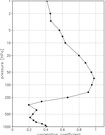
Fig. 2. Correlation coefficients of H100with <v∗T∗>N H.
Corre-lation coefficients are calculated over the years 1979–2002.
the regression of H100 with its stationary or transient wave
component represents the relative contribution by that wave component to the total variance of H100, as discussed in
Sect. 2. Table 1 shows the regression coefficients and the corresponding correlation coefficients for the total (station-ary plus transient), station(station-ary, and transient wave 1–5 compo-nents of H100. Using a Student’s t -test, we find for a sample
size of 24, that the correlation coefficient ri is significantly
different from zero at a >95%, 99%, or 99.9% confidence level if|ri| > 0.40, 0.52 or 0.63, respectively. The sum of
the regression coefficients for the total wave 1–5 contribu-tion to H100 is 0.95±0.05, with a corresponding correlation
coefficient ri=0.996 (not shown). Therefore, wavenumbers
6 and higher can be neglected in the analysis of the inter-annual variability of H100. In fact, almost all of the
inter-annual variability of H100is due to s=1–3, with a combined
regression coefficient of bi=0.96±0.06 and ri=0.98. Only
re-taining s=1,2 yields bi=0.86±0.11 and ri=0.88. We can thus
state that about 85% of the interannual variability of H100
can be attributed to its s=1,2 components. When analyzing the interannual variability of H100, it is sufficient to only
con-sider wavenumbers s=1–3, or perhaps even s=1,2. The bot-tom row of Table 1 clearly shows that the interannual vari-ability of H100 is dominated by the stationary waves, with
A. J. Haklander et al.: Interannual variability stratospheric wave driving 2579
bi=0.63±0.16 and ri=0.65. However, the correlation
coeffi-cient of H100with its transient component is also significant
at the 97.6% confidence level. 3.3 Vertical coupling
As described in the introduction, H100is proportional to the
total net wave activity flux emanating from below between 40◦N and 80◦N at the 100 hPa level. Most of the planetary wave activity that constitutes H100 has propagated upward
from its tropospheric source, and therefore, it is expected that H100 has a significant positive correlation coefficient
with the poleward eddy heat flux at levels below (and above) 100 hPa. To verify this, we examine the amount of verti-cal coupling between 100 hPa and other levels. We do this by calculating the vertical profile of the correlation coeffi-cient of H100with <v∗T∗>N H, which we define as the 20◦–
90◦N average of[v∗T∗], at levels from 1000 hPa to 1 hPa.
We compute the correlation coefficients with <v∗T∗>N H,
since the wave activity flux contributing to H100 may have
partially originated from, or may propagate into, latitudes outside the 40◦–80◦N band. The correlation coefficient pro-file is shown in Fig. 2. At 100 hPa, H100is highly correlated
with <v∗T∗>N H(r=0.95), suggesting that the 100 hPa wave
activity outside the 40◦–80◦N area is relatively small. This is confirmed by the fact that H100 accounts for about 90%
of <v∗T∗>N H at 100 hPa in the 1979–2002 period.
There-fore, to simplify the interpretation of our results, we neglect the 100 hPa upward wave activity flux at latitudes outside the 40◦–80◦N window. In Fig. 2, we see that the level of maxi-mum correlation coefficient between H100and <v∗T∗>N H
is found at 70 hPa rather than 100 hPa. Above 70 hPa, the correlation coefficient gradually decreases to marginally sig-nificant values near the stratopause∼1 hPa. Below 100 hPa, the correlation coefficient falls off quite rapidly, and is not significant (|r| <0.40) below 200 hPa. Thus, there exists a decoupling between variations in the total upward flux of wave activity in the troposphere (below 200 hPa) and vari-ations at 100 hPa. Assuming that the wave sources are pre-dominantly located in the troposphere, this decoupling can be understood as follows. Suppose an amount of wave activ-ity propagates upward in the NH at some tropospheric pres-sure level p during January–February. A fraction αp of this
wave activity is absorbed below 100 hPa, where αp lies
be-tween 0 and 1. Assuming that no wave activity crosses the equator, the remaining fraction of the wave activity (1-αp)
thus reaches the 100-hPa level and contributes to H100. If
αp is less than one and independent of time, then the
corre-lation coefficient between H100and the wave activity flux at
pressure level p will be one. On the other hand, if αp has
a large interannual variability, the correlation coefficient will be small.
For a plane and conservative planetary wave, the zonal wavenumber s and the frequency remain constant along its path (or “ray”) in the meridional plane (e.g., Karoly and
Hoskins, 1982). Therefore, it makes sense to repeat the pre-vious analysis for each individual zonal wave component. To examine the amount of vertical coupling as a function of zonal wavenumber (stationary plus transient), we compute the correlation coefficients of the wave-s component of H100
with the (same) wave-s component of <v∗T∗>N H at other
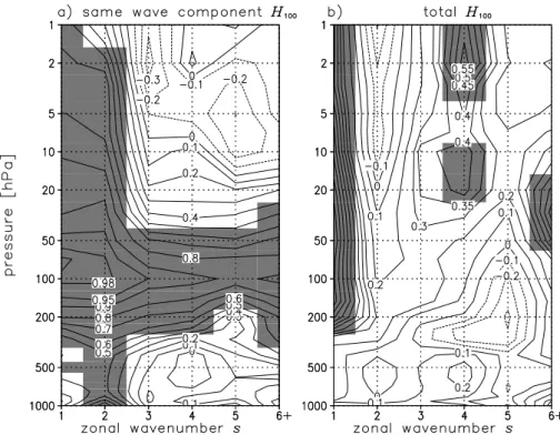
levels. We perform this analysis for the individual wavenum-bers 1 to 5 and 6+, separately. The results are shown in Fig. 3a. The s=1 component of <v∗T∗>N H is significantly
correlated with the s=1 component of H100at 500 hPa, and at
all levels above 400 hPa. The s=2 component of <v∗T∗>N H
exhibits a significant correlation with the s=2 component of
H100throughout the troposphere and the stratosphere. Note
that the wave-2 correlation coefficient reaches a minimum in the mid-troposphere but that the correlation coefficients for s=2 are statistically significant at all levels below 1 hPa. For waves with s> 2, the correlation coefficients generally only exceed the 95% significance level between 250 hPa and 50 hPa. Thus, the lack of correlation we saw in Fig. 2 be-tween the total upward flux of wave activity in the tropo-sphere and that at 100 hPa is also observed for the s>2 flux components, but not (entirely) for s=1,2. This result implies that a significant part of the interannual variability in the s = 1,2 components of H100 is due to year-to-year variations
in the strength of the s=1,2 wave source in the troposphere. There is no significant correlation for the s>2 flux compo-nents, since the refractive index for those waves exhibits a vertical layer of negative values in the lower stratosphere (Fig. 5b). Therefore, meridional refraction and reflection of the s>2 waves is taking place below 100 hPa, so that H100is
dominated by waves 1 and 2.
We have just shown that the separate s=1,2 components of H100, to which about 85% of the interannual
variabil-ity of H100 can be attributed, are significantly correlated
with the separate s=1,2 components of <v∗T∗>N H in the
troposphere. But to what extent can the interannual vari-ability of the total H100 be attributed to year-to-year
varia-tions in the separate s=1 and s=2 components (or higher) of
<v∗T∗>N H in the troposphere? To answer this question, we
examine the correlation coefficient of H100(i.e., the sum of
all wave components) with the separate wave components of
<v∗T∗>N H. The results are shown in Fig. 3b, where the
wavenumber of the pressure-dependent < v∗T∗ >N H
com-ponent is given along the horizontal axis. At levels below 200 hPa, the s=1,2 components of <v∗T∗>N H are not
sig-nificantly correlated with H100. In fact, none of the wave
components is. However, in the upper stratosphere, the s=4 component of <v∗T∗>N H exhibits a remarkably strong
cor-relation with H100. It is interesting to compare Figs. 3a and
3b. We observe in Fig. 3a that the wave-4 component of
<v∗T∗>N H in the upper stratosphere is not at all correlated
with the wave-4 component of H100. However, Fig. 3b shows
that the correlation coefficient with the total H100is highly
significant for the wave-4 component of <v∗T∗>N H in the
upper stratosphere (r=0.58 at 2 hPa, 99.7% confidence level).
Fig. 3. Correlation coefficients of (a) the zonal wave-s component of H100, and (b) H100, with the zonal wave-s component of <v∗T∗>N H.
Correlation coefficients are calculated over 1979–2002, and the areas with >95% confidence levels are shaded.
The results suggest that wavenumber 4 is a preferred mode for the breaking of very long planetary waves in the upper stratosphere.
3.4 Correlation patterns in the meridional plane
Thusfar, we have only considered averages over 40◦–80◦N and averages over the Northern Hemisphere north of 20◦N. In the previous subsection we mentioned that αp also
de-pends on the latitude at which the waves propagate upward. Therefore, we next examine where the zonal-mean upward wave-activity flux, which is proportional to[v∗T∗], is
sig-nificantly correlated with H100. The latitude- and
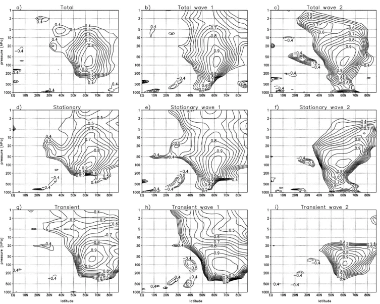
pressure-dependent correlation coefficient of H100 with [v∗T∗] is
shown in Fig. 4a. The highest correlation coefficient is found at 100 hPa and 62.5◦N (r=0.87). The decoupling between the total upward wave-activity flux at 100 hPa and that in the troposphere (Fig. 2) is also visible in Fig. 4a: H100 is not
significantly correlated with[v∗T∗] in the lower and middle
troposphere. We previously saw that the s=1,2 components of H100 significantly correlate with the same wave-s
com-ponents of <v∗T∗>N H at some level in the mid- and lower
troposphere. Figure 4b shows that the wave-1 component of H100 is significantly correlated with the wave-1
compo-nent of[v∗T∗] in the troposphere, between about 40◦N and
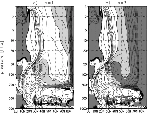
60◦N. Note that the meridionally confined correlation coeffi-cient maximum in the troposphere tilts poleward with height. A possible explanation for this correlation coefficient
maxi-mum would be the presence of a waveguide, through which the wave-1 activity is ducted to 100 hPa (e.g., Karoly and Hoskins, 1982). Since a waveguide can be identified as a ridge in the refractive index field, we verify this by comput-ing the climatological January–February pattern of the re-fractive index squared for s=1, which is shown in Fig. 5a. The wave-1 correlation coefficient maximum is roughly de-noted by the dashed line. We see that the refractive index in-deed has a ridge in the mid-latitude middle and upper tropo-sphere, which suggests that the tropospheric correlation coef-ficient maximum in Fig. 4b may be regarded as the signature of this tropospheric wave guide. To illustrate how the upper troposphere and lower stratosphere act as a low-pass filter for planetary wave activity from below, we show the refractive index field for s=3 in Fig. 5b. A mid-latitude vertical layer with negative values in the lower stratosphere emerges, of which the vertical extent increases with increasing wavenum-ber (not shown). For wavenumwavenum-ber 2 (Fig. 4c), a connection with the (lower) troposphere is found that is similar to that of wavenumber 1. A marked difference between Figs. 4c and b is, that the area of maximum correlation coefficients in the troposphere is found at higher latitudes (50–70◦N) in Fig. 4c. (The distinct and very high maximum of r=0.82 at 1000 hPa may not be very meaningful due to the extrapola-tion below ground.) This correlaextrapola-tion coefficient maximum cannot be linked to an s=2 waveguide, since the refractive in-dex field in this region is highly variable due to the presence of a zero-wind critical line, which is not sensitive to the zonal
A. J. Haklander et al.: Interannual variability stratospheric wave driving 2581
Fig. 4. Correlation coefficient of (a) H100, (b) (c) the s=1,2 component of H100, (d) the stationary component of H100, (e) (f) the stationary
s = 1,2 component of H100(g) the transient component of H100, (h), (i) the transient s=1,2 component of H100; with the same
latitude-and pressure-dependent wave component of the zonal-mean eddy heat flux averaged over January–February. Correlation coefficients are calculated over 1979–2002, and only the areas with >95% confidence levels are shown.
wave number of the refractive index. For wavenumber 2, the latitude of maximum correlation coefficients shifts equator-ward with height above 100 hPa. For the wave-3 contribution to the heat flux, the link with the troposphere is absent and the area with significant correlation coefficients is much more confined (not shown). A further decomposition into station-ary and transient wave components (Figs. 4d–i) reveals that the link with the (lower) troposphere is only statistically sig-nificant for the stationary part of the wave-1 and wave-2 con-tributions. The tropospheric meridional dipole structure in the stationary wave-1 correlation coefficient map (Fig. 4e) implies that the stationary wave-1 component of H100is
sen-sitive to the latitude of the tropospheric wave-1 source. If the source is located too far south, less wave activity is able to enter the mid-latitude waveguide and contribute to H100.
Such a dipole structure is not found in Fig. 4f for s=2.
3.5 An alternative analysis of the interannual variability of
H100
In Sect. 2.3, we mentioned an alternative way of decom-posing H100, by noting that [v∗T∗] equals the product of
rv,T with σv and σT (Eq. 4). Subsequently, we assumed
in Eq. (5) that H100 can be approximated by ˜H100. To
ex-amine the accuracy of this approximation, we first compare the 24-year averages of both ˜H100 and H100. This yields
14.1±0.4 K m s−1and 15.1± 0.5 K m s−1, respectively with a mean ratio of 0.94±0.02. To see if ˜H100 and H100 also
have comparable interannual variability, we performed a lin-ear regression of H100 with ˜H100. The regression yields a
high correlation coefficient (r=0.85) and a regression coeffi-cient b=0.71±0.09. We conclude that ˜H100is indeed a useful
approximation of H100. We next linearize the deviation of
Fig. 5. Refractive index square a2n2s in m2, based on the 1979–2002 average of the zonal-mean zonal wind during January–February, for (a)
s=1, and (b) s=3. Except for the 150 and 300 m2contours, contours are from –100 to +100 m2, with an interval of 10 m2. Negative values
are indicated by dark shading, positive values below 20 m2by light shading. The 0, 20, 40, and 150 m2contours have been labeled, and the
location of the s=1 correlation coefficient maximum is roughly denoted by the dashed line in (a).
Table 2. Linear regression of H100with σvmσTm1rv,T, σTmrv,Tm 1σv, and σvmrv,Tm 1σT at 100 hPa. The linear regression is performed over
1979–2002. The 1979–2002 averages and standard deviations are for <rv,T>, <σv>, and <σT>, respectively.
Regression coefficient Corr. coeffient 1979–2002 average 1979–2002 stdev
σvmσTm1rv,T 0.40±0.20 0.39 rv,Tm =0.23 0.04
σTmrv,Tm 1σv 0.07±0.09 0.17 σvm=10.4 m s−1 0.8 m s−1
σvmrv,Tm 1σT 0.23±0.14 0.34 σTm=5.9 K 0.7 K
˜
H100from its 1979–2002 mean as 1 ˆH100(Eq. 6). The error
1 ˆE100that arises from the linearization in Eq. (6) is
remark-ably small: a linear regression of 1 ˜H100with 1 ˆH100yields
b = 0.98±0.03 and r=0.99. The difference between 1H100
and 1 ˆH100in Eq. (7) thus primarily results from 1 ˜E100. We
can use Eq. (7) to analyze the sensitivity of H100to the
year-to-year variations in the effective phase difference <rv,T>,
as well as to the interannual variability of the effective am-plitudes <σv> and <σT>. The regression and correlation
coefficients of the linear regression analysis of H100with the
first three terms on the r.h.s. of Eq. (7) at 100 hPa are given in Table 2. The results show that the interannual variabil-ity of H100 is more sensitive to the <rv,T> than to <σv>
and <σT>. Therefore, a significant part of the year-to-year
variability in H100is not determined by variability in the
am-plitude of the waves but by variability in the efficiency of the
poleward heat transport, as represented by <rv,T>. We also
note that the variability in <σT> affects H100more strongly
than the variability in <σv>.
4 Summary and discussion
We have studied the interannual variability of the strato-spheric wave driving during NH winter, as quantified by
H100, being the January–February mean of the 40◦–80◦N
average of the total poleward heat flux at 100 hPa. For our analysis, we used 24 years (1979–2002) of ERA-40 reanal-ysis data from ECMWF. The results can be summarized as follows. We have examined the sensitivity of H100 to
sev-eral factors. The first factor is the strength of the total tropospheric wave source. It was found that H100 is not
A. J. Haklander et al.: Interannual variability stratospheric wave driving 2583 significantly correlated with the total upward wave
activ-ity flux below 200 hPa. However, both the individual zonal wave-1 and wave-2 components exhibit significant vertical coupling between 100 hPa and lower (as well as higher) lev-els. About 85% of the interannual variability of H100 can
be attributed to its s=1,2 components. However, the inter-annual variability of H100 cannot be attributed to either of
these individual wave components of the heat flux in the tro-posphere. Presumably, this is in part due to the statistically significant negative correlation coefficient that we found be-tween the s=1 and s=2 components of H100. This negative
correlation coefficient is also observed on an intraseasonal timescale, in association with the leading mode of variabil-ity in the NH winter geopotential field, the Northern An-nular Mode (NAM) (Hartmann et al., 2000). During high NAM index periods, with a stronger stratospheric polar vor-tex, the anomalous s=1 component of the heat flux at 100 hPa was negative, and the anomalous s=2 component was posi-tive. During low NAM index periods, both anomalies were of opposite sign. Thus, the negative correlation coefficient we found on the interannual timescale is also observed on the shorter timescales. The wave-1 contribution to H100was
found to depend on the latitude of the wave-1 source. Partic-ularly, if the tropospheric stationary wave-1 source is located near 30◦N instead of near 50◦N, significantly less wave ac-tivity is able to enter the mid-latitude waveguide and con-tribute to H100.
Finally, another approach was followed, where the wave driving anomalies were separated into three parts: one part due to anomalies in the zonal correlation coefficient between the eddy temperature and eddy meridional wind, another part due to anomalies in the zonal eddy temperature amplitude, and a third part due to anomalies in the zonal eddy meridional wind amplitude. It was found that year-to-year variability in the zonal correlation coefficient between the eddy tempera-ture and the eddy meridional wind is the most dominant of the three factors.
In the interpretation of our results, the assumption has been that wave activity always propagates upward, so that the source of the wave activity at 100 hPa is situated below 100 hPa. For stationary waves, this is a reasonable assump-tion. However, transient waves can develop in the strato-sphere as a result of purely stationary waves of sufficient am-plitude emanating from the troposphere, as demonstrated by Christiansen (1999). Downward propagation of these strato-spheric transients might affect H100. However, we expect this
to be only a minor influence, since the interannual variabil-ity of H100 is dominated by stationary waves (Table 1), and
transient wave activity is abundantly generated in the tropo-sphere.
In the present study, the 1958–1978 period was omitted from the analysis. However, we have also analyzed the en-tire 1958–2002 period. The results were very similar, al-though the statistical significance was generally larger due to the longer period. As a result, Fig. 3a exhibited a significant
correlation coefficient for s=1 in the entire free troposphere. A remarkable difference with the 1979–2002 analysis was found for Fig. 3b, in which the level of maximum and signif-icant correlation coefficient with H100was found to increase
with increasing wavenumber s=1–5. The s=1 correlation co-efficient decreased to statistically insignificant values of less than 0.3 in the upper stratosphere. In Fig. 4a, a clear equa-torward displacement of a statistically significant correlation coefficient maximum was observed above 100 hPa, and in Fig. 4e, the tropospheric dipole structure for s=1 in Fig. 4e was more pronounced. Finally, for the 1958–2002 period, a significantly higher refractive index was observed in the mid-latitude stratosphere for a composite with positive H100
anomalies exceeding one standard deviation than for a com-posite of negative H100 anomalies exceeding one standard
deviation. Such a significant signal could not be obtained for the 1979–2002 period, likely due to the smaller sample size. One could argue that the results depend on the 40◦–80◦N latitude window that is applied. However, replacing H100
with the NH average of[v∗T∗] at 100 hPa yields almost
iden-tical results. The present study has focused on the interannual variability of the stratospheric wave driving. We note that the factors that dominate the interannual variability may be dif-ferent from the factors that dominate the trend. These issues will be subject of our further investigation.
Acknowledgements. The authors gratefully acknowledge the
constructive suggestions that were made by the editor and three anonymous referees.
Edited by: P. Haynes
References
Andrews, D. G., Holton, J. R., and Leovy, C. B.: Middle atmo-sphere dynamics, Academic Press, 489 pp., 1987.
Austin, J., Shindell, D., Beagley, S. R., Br¨uhl, C.,Dameris, M., Manzini, E., Nagashima, T., Newman, P., Pawson, S., Pitari, G., Rozanov, E., Schnadt, C., and Shepherd, T. G.: Uncertainties and assessments of chemistry-climate models of the stratosphere, At-mos. Chem. Phys., 3, 1–27, 2003,
http://www.atmos-chem-phys.net/3/1/2003/.
Butchart, N., Scaife, A. A., Bourqui, M., de Grandpre, J., Hare, S. H. E., Kettleborough, J., Langematz, U., Manzini, E., Sassi, F., Shibata, K., Shindell, D., and Sigmond, M.: Simulations of antropogenic change in the strength of the Brewer-Dobson circu-lation, Clim. Dyn., 27, 727–741, doi:10.1007/s00382-006-0162-4, 2006.
Charney, J. G. and Drazin, P. G.: Propagation of planetary-scale disturbances from the lower to the upper atmosphere, J. Atmos. Sci., 18, 83–109, 1961.
Christiansen, B.: Stratospheric vacillations in a General Circulation Model, J. Atmos. Sci., 56, 1858–1872, 1999.
Eyring, V., Harris, N. R. P., Rex, M., Shepherd, T. G., Fahey, D. W., Amanatidis, G. T., Austin, J., Chipperfield, M. P., Dameris, M., Forster, P. M. De F., Gettelman, A., Graf, H. F., Nagashima, T., Newman, P. A., Pawson, S., Prather, M. J., Pyle, J. A., Salawitch,
R. J., Santer, B. D., and Waugh, D. W.: A strategy for process-oriented validation of coupled chemistry-climate models, Bull. Am. Meteorol. Soc., 86, 1117–1133, 2005.
Fusco, A. C. and Salby, M. L.: Interannual variations of total ozone and their relationship to variations of planetary wave activity, J. Climate, 12, 1619–1629, 1999.
Hartmann, D. J., Wallace, J. M., Limpasuvan, V., Thompson, D. W. J., and Holton, J. R.: Can ozone depletion and global warming in-teract to produce rapid climate change?, PNAS, 97, 1412–1417, 2000.
Haynes, P. H., Marks, C. J., McIntyre, M. E., Shepherd, T. G., and Shine, K. P.: On the “downward control” of extratropical diabatic circulations by eddy-induced mean zonal forces, J. Atmos. Sci., 48, 651–678, 1991.
Hu, Y. and Tung, K. K.: Possible ozone-induced long-term changes in planetary wave activity in late winter, J. Climate, 16, 3027– 3038, 2003.
Karoly, D. and Hoskins, B. J.: Three-dimensional propagation of planetary waves, J. Meteorol. Soc. Japan, 60, 109–123, 1982. Newman, P. A. and Nash, E. R.: Quantifying wave driving of the
stratosphere, J. Geophys. Res., 105, 12 485–12 497, 2000. Newman, P. A., Nash, E. R., and Rosenfield, J. E.: What controls
the temperature of the Arctic stratosphere during the spring?, J. Geophys. Res., 106(D17), 19 999–20 010, 2001.
Polvani, L. M. and Waugh, D. W.: Upward wave activity flux as pre-cursor to extreme stratospheric events and subsequent anomalous surface weather regimes, J. Climate, 17, 3548–3554, 2004.
Randel, W. J., Wu, F., and Stolarski, R.: Changes in column ozone correlated with the stratospheric EP flux, J. Meteorol. Soc. Japan, 80, 849–862, 2002.
Shepherd, T. G.: The middle atmosphere, J. Atmos. Sol.-Terr. Phys., 62, 1587–1601, 2000.
Siegmund P. C.: The generation of available potential energy: a comparison of results from a general circulation model with ob-servations, Clim. Dyn., 11, 129–140, 1995.
Sigmond, M., Siegmund, P. C., Manzini, E., and Kelder, H.: A simulation of the separate climate effects of middle atmospheric
and tropospheric CO2doubling, J. Climate, 17(12), 2352–2367,
2004.
Simmons, A. J. and Gibson, J. K.: The 40 project plan, ERA-40 Proj. Rep. Ser. 1, 63 pp., European Centre for Medium-Range Weather Forecasts, Reading, UK, 2000.
Uppala, S. M., K˚allberg, P. W., Simmons, A. J., Andrae, U., Da Costa Bechtold, V., Fiorino, M., Gibson, J. K., Haseler, J., Her-nandez, A., Kelly, G. A., Li, X., Onogi, K., Saarinen, S., Sokka, N., Allan, R. P., Andersson, E., Arpe, K., Balmaseda, M. A., Beljaars, A. C. M., Van De Berg, L., Bidlot, J., Bormann, N., Caires, S., Chevallier, F., Dethof, A. ,Dragosavac, M., Fisher, M., Fuentes, M., Hagemann, S., H´olm, E., Hoskins, B. J., Isaksen, L., Janssen, P. A. E. M., Jenne, R., McNall, A. P. Y., Mahfouf, J.-F., Morcrette, J.-J., Rayner, N. A., Saunders, R. W., Simon, P., Sterl, A., Trenberth, K. E., Untch, A., Vasiljevic, D., Viterbo, P., and Woollen, J.: The ERA-40 re-analysis, Quart. J. R. Meteorol. Soc., 131, 2961–3012, doi:10.1256/qj.04.176, 2005.