HAL Id: hal-00318107
https://hal.archives-ouvertes.fr/hal-00318107
Submitted on 23 Dec 2005
HAL is a multi-disciplinary open access
archive for the deposit and dissemination of
sci-entific research documents, whether they are
pub-lished or not. The documents may come from
teaching and research institutions in France or
abroad, or from public or private research centers.
L’archive ouverte pluridisciplinaire HAL, est
destinée au dépôt et à la diffusion de documents
scientifiques de niveau recherche, publiés ou non,
émanant des établissements d’enseignement et de
recherche français ou étrangers, des laboratoires
publics ou privés.
divergent ray trajectories and ground accessibility
J. Chum, O. Santolik
To cite this version:
J. Chum, O. Santolik. Propagation of whistler-mode chorus to low altitudes: divergent ray trajectories
and ground accessibility. Annales Geophysicae, European Geosciences Union, 2005, 23 (12),
pp.3727-3738. �hal-00318107�
Annales Geophysicae, 23, 3727–3738, 2005 SRef-ID: 1432-0576/ag/2005-23-3727 © European Geosciences Union 2005
Annales
Geophysicae
Propagation of whistler-mode chorus to low altitudes: divergent ray
trajectories and ground accessibility
J. Chum1and O. Santol´ık2,1
1Institute of Atmospheric Physics, Bocni II/1401, 14131 Praha 4, Czech Republic
2Charles University, Faculty of Mathematics and Physics, V Holesovickach 2, 18000 Praha 8, Czech Republic Received: 23 June 2005 – Revised: 20 October 2005 – Accepted: 8 November 2005 – Published: 23 December 2005
Abstract. We investigate the ray trajectories of nonductedly
propagating lower-band chorus waves with respect to their initial angle θ0, between the wave vector and ambient mag-netic field. Although we consider a wide range of initial an-gles θ0, in order to be consistent with recent satellite obser-vations, we pay special attention to the intervals of initial an-gles θ0, for which the waves propagate along the field lines in the source region, i.e. we mainly focus on waves generated with θ0within an interval close to 0◦and on waves generated within an interval close to the Gendrin angle. We demon-strate that the ray trajectories of waves generated within an interval close to the Gendrin angle with a wave vector di-rected towards the lower L-shells (to the Earth) significantly diverge at the frequencies typical for the lower-band chorus. Some of these diverging trajectories reach the topside iono-sphere having θ close to 0◦; thus, a part of the energy may leak to the ground at higher altitudes where the field lines have a nearly vertical direction. The waves generated with different initial angles are reflected. A small variation of the initial wave normal angle thus very dramatically changes the behaviour of the resulting ray. Although our approach is rather theoretical, based on the ray tracing simulation, we show that the initial angle θ0of the waves reaching the iono-sphere (possibly ground) is surprisingly close – differs just by several degrees from the initial angles which fits the ob-servation of magnetospherically reflected chorus revealed by CLUSTER satellites. We also mention observations of di-verging trajectories on low altitude satellites.
Keywords. Magnetospheric physics (Waves in plasma) –
Space plasma physics (Wave-particle interactions, Waves and instabilities) – Ionosphere (Wave propagation)
1 Introduction
Together with the lightning induced whistlers, chorus emis-sions belong to the most distinct electromagnetic waves propagating in the inner magnetosphere. Chorus was first
Correspondence to: J. Chum
(jch@ufa.cas.cz)
observed on the ground (Storey, 1953). Later its investiga-tion has mainly been based on the satellite measurements. Chorus propagates as whistler mode plasma waves and con-sists of narrowband tones usually rising (sometimes falling) in frequency on the time scale of several tenths of a sec-ond. Near the magnetic equator, chorus occurs usually in two distinct frequency bands separated by a narrow gap at one half of the electron cyclotron frequency ωceq (Tsurutani and Smith, 1974), with the upper-band just above the half of ωceq (ω/ωceq∼0.5−0.6), and the lower band in the range (ω/ωceq∼0.2–0.45).
The satellite measurements have recently brought new pieces of knowledge about chorus properties. The Poynt-ing flux measurement on Polar (LeDocq et al., 1998) and the CLUSTER satellites (Parrot et al., 2003) have confirmed the previous suggestion by Helliwel (1967, 1969), that the cho-rus source is located close to the magnetic equatorial plane, with the dimension along magnetic field line being up to sev-eral thousands of kilometres, thus expanding a few degrees from the magnetic equator (Santol´ık et al., 2005). The cross-correlation of spectrograms recorded on different CLUSTER satellites have shown that the transverse dimension (with re-spect to magnetic field) of the source located at the magnetic equator could be lower than 100 km (Santol´ık et al., 2004) in the case of lower band chorus. Beyond that distance the cor-relation coefficient calculated from the spectrograms rapidly decreases.
The detailed understanding of the generation mechanism is still a subject of active research. It is generally believed that the generation of chorus emissions is driven by the in-jection of substorm electrons (Tsurutani and Smith, 1974; Bespalov and Trakhengerts, 1986) that interact with whistler mode waves through the cyclotron resonance (Andronov and Trakhtengerts, 1964; Kennel and Petschek, 1966). However, the linear theory cannot clarify the discrete character of the chorus elements. Several authors have attempted to explain the main properties of the chorus emission, such as the re-currence rate and the slope of the chorus elements (tones). Trakhtengerts (1995, 1999) used a theory of the backward wave oscillator in the ELF/VLF frequency band. According to his theory, a step-like electron distribution function, which
is formed as a result of the development of a cyclotron insta-bility, leads to an absolute instability and the wave generation in the form of discrete elements with rising frequency. Nunn et al. (1997) considered that a strong nonlinear phase trap-ping of cyclotron resonant electrons is the essential mech-anism producing the VLF chorus. Using the Vlasov code simulation in 4-D phase space, Nunn (2004) was able to re-produce the main properties of chorus.
Originally, the chorus properties have been studied under the assumption of ducted propagation of the emission from the source. This assumption has been supported by the fact that chorus emissions can be observed on the ground. Next, it has generally been accepted that the lower band chorus is generated with wave vectors directed close to the magnetic field lines. The latter assumption is also based on the satellite measurements carried out close to the source region, which show that the mean value of wave normal angle θ0is usu-ally small, close to zero (Nagano et al., 1996). However, the first identification of magnetospherically reflected (MR) cho-rus described by Parrot et al. (2003), and the plasma density measurements show that, in many cases, there are no ducts and chorus emissions may propagate obliquely with respect to magnetic field lines. The detailed ray tracing analysis of the MR chorus shows that the emission has to be generated with relatively large wave normal angles θ0to the magnetic field line (Parrot et al., 2004), with the wave vector directed towards the Earth. Chum et al. (2003) showed, under the assumption of nonducted propagation, that a span of wave normal angles should exist in the generation region, so that it would be possible to observe a chorus element at higher latitudes.
Applying the ray tracing analysis to the frequencies that are typically observed both on the satellites and on the ground and assuming nonducted propagation, we will show that for specific values of initial angle θ0, a relatively small change in the initial angle θ0 leads to the distinctly differ-ent wave trajectories and to the divergence of wave normal angles along these trajectories. We will demonstrate that the divergence occurs for waves generated at relatively large angles, with wave vectors directed towards lower L-shells (the Earth). Some of these waves may reach the topside ionosphere with θ ∼0, thus probably leaking to the ground, whereas the waves generated with sufficiently different ini-tial θ0, including those generated along the field line, un-dergo the magnetospheric reflection.
In the present paper we concentrate on a detailed theoret-ical ray tracing analysis of this problem. In a related experi-mental paper (Santol´ık et al., 20051), we present an interpre-tation of spacecraft observations of the divergent propagation pattern at high latitudes.
1Santol´ık, O., Chum J., Parrot M., Gurnett, D. A., Pickett, J. S., and Cornilleau-Wehrlin, N.: Propagation of whistler-mode chorus to low altitudes: Spacecraft observations of structured ELF hiss, J. Geophys. Res., submitted, doi:2005JA011462, 2005.
2 Convergence and divergence of ray trajectories; ground accessibility and magnetospheric reflection; results of ray tracing simulation
2.1 Ray tracing
In this section we will investigate the ray trajectories of lower band chorus waves for a wide range of initial angles θ0 be-tween the wave vector and magnetic field line. The ray trac-ing software that we use is based on the dipole magnetic field model, which means that the cyclotron frequency ωcis given by expression (1)
ωc=ωc0·
(1 + 3· sin2λ)1/2 (R/RE)3
, (1)
where ωc0 is the electron cyclotron frequency at the mag-netic equator on the Earth’s surface, λ is magmag-netic latitude, |R|=L· cos2(λ), and L is the distance of magnetic field line from the Earth’s centre in the magnetic equator plane, in Earth radii (RE).
In order to verify the robustness of the acquired results, we have used two different packages of ray tracing software and compared the results. The first software uses a gyrotropic distribution of plasma density (plasma frequency ωp, re-spectively), that is ω2p∝ωnc(n∼1), and an approximation of the general dispersion relation in cold magnetized plasmas, which is valid only in the frequency range ωci ω≤ωc·cos θ (ωci is ion cyclotron frequency), and in a dense plasma, ω2p ω2c. The latter inequality holds in most of the magne-tosphere, except for the polar region. The effect of ions on whistler mode wave propagation is in the approximation of the dispersion relation (Eq. 2) included via the Lower Hybrid Resonance (LHR) frequency ωLH. ω2= ω 2 LH 1 + ωp2 k2·c2 + ω 2 c·cos2θ (1 + ω2p k2·c2)2 , (2)
where c is speed of light and k is the modulus of the wave vector. An analytic model of LHR frequency, which repro-duces the main features of the LHR frequency in the plas-masphere is used. More details can be found in Shklyar and Jiricek (2000).
The second ray tracing software uses a diffusive equilib-rium model of plasma density distribution, defined by the balance of the thermal pressure and gravitational forces. A temperature of 1000 K at the reference level of 1000 km has been used in this paper as a basis for the density model, together with predefined ratios of the plasma frequency to the electron cyclotron frequency in the chorus source re-gion. Another difference compared to the previous ray-tracing software is that we do not use approximative ex-pressions for the dispersion relation, but an exact solution to the dispersion relation in cold plasmas, taking into ac-count both electron and ion contributions (Stix, 1992). Sev-eral ion species can be taken into account but only a hy-drogen plasma is used in the present paper. The rays are generally followed in three dimensions, but this capability
J. Chum and O. Santol´ık: Propagation of whistler-mode chorus to low altitudes 3729
12
Fig. 1: Ray tracing analysis of 2.5 kHz waves for 7 different initial angles generated at
L=4.85. The gyrotropic model of plasma density distribution was used. Colours discern the
different initial angles
θ
0; the values of initial angles are written in the right bottom plot.
Left column: ray trajectories in different coordinate systems; upper plot: in the meridian plane
(xz plane, the z axis corresponds to the axis of Earth’s magnetic dipole), underneath: in
magnetic latitude and L shell coordinates. Right column: evolution of the refractive index as a
function of time (on top), wave normal angle
θ
as a function of magnetic latitude (on the
bottom).
Here and further, the notation is the following:
θ =0 means that the wave propagates along the
field line towards southern hemisphere, the “+” sign stands for waves having the wave vector
directed towards the higher L-shells,
θ =180
orepresents the wave propagating along the filed
line towards the northern hemisphere.
In the top left plot, the thick cyan colour indicates contour of
ω
LH=2.5 kHz. In the bottom left
plot, the blue, green and brown lines represent the equatorial electron cyclotron frequency of
5 kHz, 7.5 kHz and 10 kHz.
.
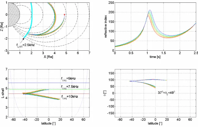
Fig. 1. Ray tracing analysis of 2.5 kHz waves for 7 different initial angles generated at L=4.85. The gyrotropic model of plasma density
distribution was used. Colours discern the different initial angles θ0; the values of the initial angles are written in the right bottom plot. Left column: ray trajectories in different coordinate systems; upper plot: in the meridian plane (xz plane, the z axis corresponds to the axis of the Earth’s magnetic dipole), underneath: in magnetic latitude and L-shell coordinates. Right column: evolution of the refractive index as a function of time (on top), wave normal angle θ as a function of magnetic latitude (on the bottom). Here and further, the notation is the following: θ =0 means that the wave propagates along the field line towards the Southern Hemisphere, the “+” sign stands for waves having the wave vector directed towards the higher L-shells, θ =180◦represents the wave propagating along the field line towards the Northern Hemisphere. In the top left plot, the thick cyan colour indicates the contour of ωLH=2.5 kHz. In the bottom left plot, the blue, green and brown lines represent the equatorial electron cyclotron frequency of 5 kHz, 7.5 kHz and 10 kHz.
is not used here, and only two-dimensional calculations in the local magnetic meridian plane are performed. The ba-sic properties of this software were presented by Cairo and Lefeuvre (1986). Compared to this described version, the al-gorithm of the integration of differential equations of the ray trajectories has been rewritten, using the Runge-Kutta 4th or-der method with one midpoint and an adaptive integration step. Additionally, wave-mode control and integration stop criteria have been modified. The Wentzel-Kramers-Brillouin (WKB) approximation of geometric optics is verified in ev-ery integration step and the ray is not followed beyond the limit where this basic approximation becomes invalid. 2.2 Magnetospheric reflection
Before we start the ray tracing simulation, it is instructive to keep in mind the basic characteristics of a magnetospheric reflection (MR), which is actually, strictly speaking, a refrac-tion. Although it is related to the LHR frequency, it doesn’t occur exactly at the point where the wave frequency equals the local LHR frequency ω=ωLH, as it is often stated for simplicity, but may also happen at frequencies well below
this value. The detailed analysis has recently been made by Shklyar et al. (2004), who studied the MR lightning induced whistlers observed close to the reflection region. Shklyar et al. (2004) showed that the reversal of the direction of the group velocity is mainly due to the reversal of its parallel component (with respect to the magnetic field), which takes place at the frequency ω, given by Eq. (3), which may be obtained from the definition of group velocity and Eq. (2): ω2= ω 2 LH 1 + ω 2 p k2·c2 . (3)
From Eq. (3), it is obvious that the frequency ω, at which the parallel component of the group velocity reverses, is al-ways less than the local LHR frequency (ω<ωLH), and ap-proaches the LHR frequency as the wave number increases, being approximately equal to it for waves propagating close to the resonance cone.
2.3 Initial conditions and assumptions
The initial conditions and assumptions in our analysis are the following:
13
Fig. 2: Ray tracing analysis of 2.5 kHz waves generated at L=4.85 having the initial angles
along the field line in the range -6
o≤ θ ≤ +6
o, that is, with the wave vector initially directed
along the field line. The gyrotropic model of plasma density distribution was used. We can
see that these rays undergo magnetospheric reflection and don’t diverge significantly. The
rays also don’t change the initial L shell distinctly. The colours change with increasing initial
angle
θ similarly as in Figure 1.
Fig. 2. Ray tracing analysis of 2.5 kHz waves generated at L=4.85 having the initial angles along the field line in the range −6◦≤θ ≤+6◦, that is, with the wave vector initially directed along the field line. The gyrotropic model of plasma density distribution was used. We can see that these rays undergo magnetospheric reflection and don’t diverge significantly. The rays also don’t change the initial L-shell distinctly. The colours change with increasing initial angle θ , similarly as in Fig. 1.
– Nonducted propagation; there are no sharp density
gra-dients;
– A small transverse dimension of the source region
(San-tol´ık and Gurnett, 2003);
– There is a span of initial wave normal angles θ0in the source region;
– We will show the analysis for two different frequencies:
2.5 kHz and 575 Hz. Initially, the gyrotropic model of plasma density distribution is applied in the analysis, however, the main subject of this paper, the divergence of trajectories, is presented for the two different models of plasma density distribution, in order to demonstrate the robustness of the result.
2.4 Ray trajectories for a wide range of initial angles θ0 We will start with waves of frequency 2.5 kHz that are com-monly observed both at ground stations and on satellites. Burtis and Helliwell (1976) have found in their statistical survey based on OGO 3 data that the normalized frequency distribution of mean chorus frequency has a peak slightly above f/fc=1/3 in the equatorial region (fc is the electron cyclotron frequency). Therefore, we will start our simula-tion in such a way that the initial ratio of f/fcat the equator
is close to that peak, (f/fc=0.328 in our case), at L=4.85. The important angles at the equator are the following: the resonance angle θR=70.85◦,the Gendrin angle θG=49◦.
First we study the ray trajectories for a wide interval of initial angles θ0, from −63◦to +63◦in the meridian plane. The “+” sign means that the wave vector is directed to higher L-shells (from the Earth). The simulation was first done for seven θ0 values with a relatively large step of 21◦, so that we could easily distinguish the trajectories. The results are presented in Fig. 1; different colours are used to discern the trajectories corresponding to the different initial angles θ0. We can see that for most initial angles, the waves undergo magnetospheric reflection close to the region, where their frequency matches the LHR frequency. Note that even the waves which have been initially started along the field line (θ0=0) do reflect magnetospherically. It can, however, be difficult to observe these reflected waves, because their tra-jectories merge with the tratra-jectories of the more intense di-rect waves. Although there may be a transitional behaviour due to the existence of the Gendrin angle, we can see that the final L-shell usually decreases with an increasing initial an-gle θ0(including the sign). There is, however, an exception for a large negative initial angle θ0. The trajectories started with initial angles θ0 between −63◦, and −42◦ are highly diverging (not shown). It should also be noted that the di-vergence is well expressed in the evolution of wave normal
J. Chum and O. Santol´ık: Propagation of whistler-mode chorus to low altitudes 3731
14
Fig. 3: Ray tracing analysis of 2.5 kHz waves generated at L=4.85 having the initial angles in
the interval 37
o≤ θ ≤ 49
o(
θ
G-12
o≤ θ ≤ θ
G), that is with the wave vector initially directed
from the Earth, towards the higher L-shells. The gyrotropic model of plasma density
distribution was used. We can see that the rays converge. The rays undergo the
magnetospheric reflection as well. Remarkable is also the decrease of L-shell during the
propagation. At higher latitudes, the frequency normalized to the equatorial electron cyclotron
frequency is about ¼. In the equatorial region, the rays propagate along the field line. The
usage of colours is the same as in the previous figures.
Fig. 3. Ray tracing analysis of 2.5 kHz waves generated at L=4.85 having the initial angles in the interval 37◦≤θ ≤49◦(θG−12◦≤θ ≤θG), that is, with the wave vector initially directed from the Earth, towards the higher L-shells. The gyrotropic model of plasma density distribution was used. We can see that the rays converge. The rays undergo the magnetospheric reflection, as well. Also remarkable is the decrease in the L-shell during propagation. At higher latitudes, the frequency normalized to the equatorial electron cyclotron frequency is about 1/4. In the equatorial region, the rays propagate along the field line. The usage of colour is the same as in the previous figures.
angles θ along the trajectories, as well (right bottom plot). Another important feature is that these diverging trajectories arrive close to the topside ionosphere. The divergence of tra-jectories will be studied in more detail in the next subsection. Note also that except the interval of initial angles corre-sponding to the diverging trajectories, the higher (positive) angle θ0that we choose, the lower the L-shell of the ray tra-jectory at higher altitudes or after the magnetospheric reflec-tion.
2.5 Ray trajectories of waves generated with group velocity along the field line
Santol´ık and Gurnet (2003), in their correlation analysis of chorus wave packets recorded on different CLUSTER satel-lites in the generation region, assumed that the emissions propagate along the field line in the equatorial region. This is also consistent with the theoretical assumption that there should be a sufficient length of interaction region, in which the waves propagate antiparallel to energetic electrons, so that the feedback between waves and particles could oper-ate to produce discrete emissions. Usually a generation with wave vector along the field line is considered (e.g. Trakht-engerts, 1995, 1999; Nunn, 2004). However, the genera-tion with a wave vector deviated from the field line to a value, which is close to the Gendrin angle (Gendrin, 1961)
also results in the wave propagating along the field line in the generation region. More precisely, to ensure the initial propagation along the field line, the waves should be gener-ated with angles a little bit smaller than the Gendrin angle, since the wave normal angle θ always tends to increase near the equatorial region during the nonducted propagation (see, for example, Figs. 1–5). In the following, we will analyse all three possible situations in the meridian plane: genera-tion along the field line, generagenera-tion close to the Gendrin an-gle with a wave vector directed to higher L-shells (from the Earth) and with the wave vector directed to the lower L-shells (toward the Earth). The results of the ray tracing simulations for waves of frequency 2.5 kHz are presented in Figs. 2, 3, 4 (for the gyrotropic model of the plasma density distribu-tion) and in Fig. 5 (for the diffusive equilibrium model of the plasma density distribution). Comparing the results of these simulations, we can see that the waves which started with positive angles θ (Fig. 3) exhibit the highest refractive index from these three possibilities of different intervals of initial angles θ0. They also converge most significantly; their ray bundle width is the smallest. Their energy density is thus the highest, especially in the electric component. Since their re-fractive index is high, it is probable that these waves would be damped significantly. They undergo the magnetospheric reflection in the region, where their frequency is very close
15
Fig. 4: Ray tracing analysis of 2.5 kHz waves generated at L=4.85 having the initial angles
in the interval -63
o≤ θ ≤ −51
o. The gyrotropic model of plasma density distribution was used.
The divergence of ray trajectories and divergence of evolution of wave normal angles along
these trajectories can be clearly seen. Most of the waves reach the topside ionosphere; thus a
part of their energy may possibly leak to the ground. The waves reaching the height of ~300
km are artificially reflected in the simulation. The proper treatment of trajectories of these
waves would require the full wave solution. The usage of colours is the same as in the
previous figures.
Fig. 5: The same as in Figure 4, but for the diffusive
equilibrium model of plasma density
distribution.
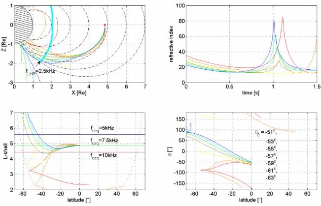
Fig. 4. Ray tracing analysis of 2.5 kHz waves generated at L=4.85 having the initial angles in the interval −63◦≤θ ≤−51◦. The gyrotropic model of plasma density distribution was used. The divergence of ray trajectories and the divergence of the evolution of wave normal angles along these trajectories can be clearly seen. Most of the waves reach the topside ionosphere; thus, a part of their energy may possibly leak to the ground. The waves reaching the height of ∼300 km are artificially reflected in the simulation. The proper treatment of trajectories of these waves would require the full wave solution. The usage of colour is the same as in the previous figures.
to the local LHR frequency. The L-shell decreases substan-tially during propagation, except for the generation region. We should stress that the waves generated along the field lines are also magnetospherically reflected. However, they don’t change the L-shell significantly (Fig. 2).
Starting with the wave vector directed significantly to-wards the lower L-shells we obtain completely different be-haviour of the trajectories. The result of the simulation is in Fig. 4 (gyrotropic model of the distribution of plasma den-sity) and in Fig. 5 (diffusive equilibrium model of plasma density distribution). First of all, we notice the remarkable divergence of the trajectories. Additionally, some of the waves generated with negative angles θ reach the topside ionosphere with relatively low angles θ . Note that the ray trajectories are shown only for selected initial angles. How-ever, all the trajectories between the displayed ones in the selected interval are considered in the discussions through-out the paper.
If the waves propagate approximately perpendicularly to the bottom boundary of the ionosphere, they can fulfill the condition for refraction/mode transfer to the “free space” electromagnetic waves, and reach the ground. If we assume, for simplicity, that the boundary between the bottom side of the ionosphere and the non-ionised atmosphere is a flat plane, then the boundary condition requires the tangential compo-nents of electric and magnetic fields to be continuous at this
boundary. Under another assumption that the regions on both sides of the boundary can be considered as homogenous (the wave vector changes significantly on scales much larger than the wavelength), we can simply apply Snell’s law, which states the equality for the tangential components of the re-fractive index N . Since the value of the rere-fractive index in the non-ionised atmosphere is ∼1, the value of the tangen-tial component of the refractive index (with respect to the boundary) of the incident wave should also be close to ∼1. Assuming that the boundary is parallel to the Earth’s surface, and using the dispersion relation and proper plasma density, it is possible to estimate the maximum deviation of the wave vector from the vertical direction in the ionosphere, which can have the waves reaching the ground. (See also Fig. 6, presenting the components of refractive index in a magne-tised cold plasma.) The waves propagating at higher angles to the vertical direction undergo the reflection back to the ionosphere. Thus, a small wave-normal angle with respect to the vertical direction prevents the ionospheric reflection, while a small angle to the magnetic field line prevents the magnetospheric reflection. It is obvious that both require-ments can be fulfilled at higher magnetic latitudes, where the field and vertical direction are close to each other. In real-ity, the rapid change in the wave vector in the ionosphere might break the limitation of geometrical optics, and the ex-act treatments of such waves would require the full wave
J. Chum and O. Santol´ık: Propagation of whistler-mode chorus to low altitudes 3733
15
Fig. 4: Ray tracing analysis of 2.5 kHz waves generated at L=4.85 having the initial angles
in the interval -63
o≤ θ ≤ −51
o. The gyrotropic model of plasma density distribution was used.
The divergence of ray trajectories and divergence of evolution of wave normal angles along
these trajectories can be clearly seen. Most of the waves reach the topside ionosphere; thus a
part of their energy may possibly leak to the ground. The waves reaching the height of ~300
km are artificially reflected in the simulation. The proper treatment of trajectories of these
waves would require the full wave solution. The usage of colours is the same as in the
previous figures.
Fig. 5: The same as in Figure 4, but for the diffusive
equilibrium model of plasma density
distribution.
Fig. 5. The same as in Fig. 4, but for the diffusive equilibrium model of plasma density distribution.
solution. In the simulation, the waves reaching the height of 300 km are artificially reflected in Fig. 4. For the waves of frequencies below the proton cyclotron frequency the situa-tion is even more complicated, and the multi-ion cutoff (Gur-nett and Burns, 1968) should be considered for waves which do not propagate along the field line. The scattering on the irregularities in the ionosphere is also possible.
Let us call the bifurcation angle θBthe initial angle θ0, for which the trajectories arrive at the topside ionosphere with θ=0. In the case presented in Fig. 4, the bifurcation angle is a little bit less than −59◦. If we use the diffusive equi-librium model (Fig. 5), the bifurcation angle is a little bit less than –60◦. From the simulation, it is obvious that if the initial angle approaches the bifurcation angle the trajec-tories tend to diverge most significantly. For the initial angle θ0>θBthe trajectories tend to reflect towards higher L-shells, whereas for the θ0<θBthe trajectories tend to reflect towards lower L-shells. Of course, the bifurcation angle depends on the plasma density distribution, and the starting point from which we investigate the trajectories.
The existence of the bifurcation angle (divergence) of the trajectories is a consequence of the rather complicated de-pendence of the direction of the group velocity on the angle θ, and the evolution of the wave vector along the ray tra-jectories for these initial conditions. For the clearness of further discussion, Fig. 6 displays the contours of ω=const in the (N⊥, N||)space, or, in other words, the dependence of the refractive index (wave vector) on the angle θ . The ray direction (direction of group velocity) can be found as the normal to this curve in a given point. The remarkable
divergence and/or “temporally” convergence of the trajecto-ries can be observed if the ray bundle consists of waves hav-ing angles around θ =0 and/or around θ =θG; the latter possi-bility only exists in the frequency range ωLH<ω<ωc/2. The first case (θ =0) usually leads to the divergence of the trajec-tories (provided that ω<ωc/2) in the Earth’s magnetosphere, whereas the occurrence of the second case (θ ∼θG)is often connected with the intersection of the trajectories. Return-ing to our simulation results, we can see this intersection at latitudes from ∼−20◦to −25◦in Figs. 4 and 5. At higher lat-itudes and lower altlat-itudes the waves reach the region where their frequency is ω<ωLH, and they tend to reflect magne-tospherically if their wave-normal angle is sufficiently high (Sect. 2.2). Some waves from the ray bundle propagate to the region where their frequency is considerably lower than ωLH and the evolution of their wave normal angle inherently tends to 0. All the other waves have a distinct tendency to reflect/to shift their wave vectors into the perpendicular direction to magnetic field lines. Simultaneously, we can observe an ex-tremely remarkable divergent propagation; the evolution of wave-normal angles is highly divergent, as well. This is what we call divergence further on in this paper, though the trajec-tories are diverging, in fact, from the beginning. The most distinct divergence occurs for waves whose initial angles ap-proach the value of the bifurcation angle. Note that for most of the initial angles there is also an overall tendency of the oblique whistler mode wave to steer its wave vector towards higher L-shells as it propagates from the equator in the inner magnetosphere (see, for example, Fig. 1).
16
Fig. 6: Contours of
ω=const in the space of perpendicular (N
⊥) and parallel (N
||) components
of the refractive index with respect to the magnetic field line. Direction of the group velocity
is given by the normal to these contours. Left plot displays the situation for the frequency
range
ω
LH<
ω < ω
c/2; the right plot shows the case for frequencies
ω
ci<
ω < ω
LH. Note that the
scale is different in both plots and axis. Both plots were computed under assumption
ω
p/ω
c=5.
.
Fig. 7: Ray tracing analysis of MR chorus observed by Parrot et al. (2003). The gyrotropic
model of plasma density distribution was used. The analysis was started at the equator at
L=6.7. The initial angles are in the interval -70.5
o≤
θ
≤ −
67.5
o. The usage of colours is the
same as in the previous figures. That means, for example red line stands for
θ
0=
−
70.5
o, blue
line stands for -67.5
o, olive line stands for –69
o.
Fig. 6. Contours of ω=const in the space of perpendicular (N⊥) and parallel (N||)components of the refractive index with respect to the magnetic field line. The direction of the group velocity is given by the normal to these contours. Left plot displays the situation for the frequency range ωLH<ω<ωc/2; the right plot shows the case for frequencies ωci<ω<ωLH. Note that the scale is different in both plots and axis. Both plots were computed under the assumption ωp/ωc=5.
16
Fig. 6: Contours of
ω=const in the space of perpendicular (N
⊥) and parallel (N
||) components
of the refractive index with respect to the magnetic field line. Direction of the group velocity
is given by the normal to these contours. Left plot displays the situation for the frequency
range
ω
LH<ω < ω
c/2; the right plot shows the case for frequencies
ω
ci<ω < ω
LH. Note that the
scale is different in both plots and axis. Both plots were computed under assumption
ω
p/ω
c=5.
.
Fig. 7: Ray tracing analysis of MR chorus observed by Parrot et al. (2003). The gyrotropic
model of plasma density distribution was used. The analysis was started at the equator at
L=6.7. The initial angles are in the interval -70.5
o≤
θ
≤ −
67.5
o. The usage of colours is the
same as in the previous figures. That means, for example red line stands for
θ
0=−
70.5
o, blue
line stands for -67.5
o, olive line stands for –69
o.
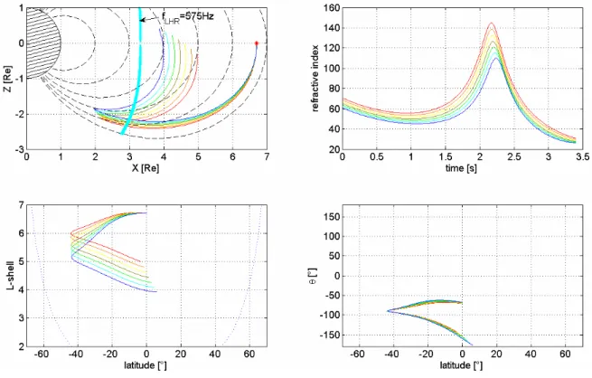
Fig. 7. Ray tracing analysis of MR chorus observed by Parrot et al. (2003). The gyrotropic model of plasma density distribution was used.
The analysis was started at the equator at L=6.7. The initial angles are in the interval −70.5◦≤θ ≤−67.5◦. The usage of colour is the same as in the previous figures. This means, for example, red line stands for θ0=−70.5◦, the blue line stands for −67.5◦, the olive line stands for
−69◦.
2.6 Observed MR chorus and divergence of ray trajectories
The bifurcation angle, introduced in the previous paragraph, is close to the Gendrin angle and corresponds to wave vec-tors directed towards the lower L-shells (to the Earth). Al-though the main portion of chorus energy could be gener-ated in different wave vector directions, it is surprising that
similar initial conditions give the ray trajectories that corre-spond to the observation of MR chorus described by Parrot et al. (2003). Therefore, we will continue with the ray tracing analysis of MR chorus observed simultaneously with direct chorus (propagating from the equator) by Parrot et al. (2003). Let us shortly summarize the facts: the direct chorus waves were observed on the CLUSTER satellites at a radial distance
J. Chum and O. Santol´ık: Propagation of whistler-mode chorus to low altitudes 3735
17
Fig. 8: Ray tracing analysis of 575 Hz waves started at the same place as in Fig. 7, but having
the range of initial angles -66
o≤
θ
≤ −54
o. The gyrotropic model of plasma density
distribution was used. The divergence of ray trajectories and the divergence of wave normal
angles along the ray trajectories can be clearly seen. The colours again indicate the different
initial angles
θ
0. Assignment of colours is obvious from the right-hand panel at the bottom;
the system is the same as in the previous figures. The waves reaching the height of 300 km are
artificially reflected in the simulation. The proper treatment of trajectories of waves reaching
the topside ionosphere would require a full wave approach.
Fig. 9: The same as in Figure 8, but for the diffusive equilibrium model of the plasma density
distribution.
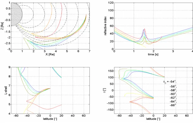
Fig. 8. Ray tracing analysis of 575 Hz waves starting at the same place as in Fig. 7, but having the range of initial angles −66◦≤θ ≤−54◦. The gyrotropic model of plasma density distribution was used. The divergence of ray trajectories and the divergence of wave normal angles along the ray trajectories can be clearly seen. The colours again indicate the different initial angles θ0. Assignment of colours is obvious from the right-hand panel at the bottom; the system is the same as in the previous figures. The waves reaching the height of 300 km are artificially reflected in the simulation. The proper treatment of trajectories of waves reaching the topside ionosphere would require a full wave approach.
of 4.5 RE (RE is the Earth’s radius) and magnetic latitude MLAT∼35◦(L∼6.7), simultaneously with MR chorus (2–3 orders weaker) at R∼4.4 and MLAT∼10◦(L∼4.5). All satel-lites were located close to one single meridian plane. The result of the simulation (in the meridian plane) that more or less fits this observation is graphically shown in Fig. 7. The waves of frequency 575 Hz were launched at the magnetic equator at L=6.7 within the range of initial wave normal angles −70.5◦≤θ0≤−67.5◦. The model electron cyclotron frequency at the equator is 2.89 kHz; thus, the initial ratio f/fc=0.1989 at the equator is distinctly lower than in the pre-vious case. The resonance angle θR∼acos(f/fc), and the Gen-drin angle θG∼acos(2f/fc) at the equator are the following: θR=78.53◦, θG=66.56◦. We can see that after the initial phase, when the rays propagate approximately along the field line, the rays undergo a rapid decrease in the L-shell (the bottom panel on the left) and return to the equator propagat-ing almost anti-parallel to the magnetic field lines.
Worth noticing is also the fact that the trajectories are quite sensitive to the initial angle θ0, although the divergence of trajectories is not so distinct as it was in the case presented in Figs. 4 and 5. Now there is nearly no divergence of angle θ along the trajectories. Nevertheless, based on the experience with the previous analysis for waves of frequency 2.5 kHz, it is reasonable to suppose that the highly divergent pattern
may occur for initial angles θ0which are not too far from the interval −70.5◦≤θ0≤−67.5◦. Indeed, the simulations pre-sented in Fig. 8 (gyrotropic model of plasma distribution) and in Fig. 9 (diffusive equilibrium model of plasma distri-bution) show that also in these cases we can find a highly divergent pattern both in the trajectories and in the wave nor-mal angle θ . The bifurcation angle is approximately −60◦ for the gyrotropic model, or somewhat more than −62◦ in the case of the diffusive equilibrium model of the plasma density distribution. In both cases, these angles are not too far from the initial angle corresponding to chorus rays shown in Fig. 7, which fit rather well the observations of MR chorus described by Parrot et al. (2003), and at the same time, from the value of the Gendrin angle (θG=66.56◦).
Note that, for initial angles θ0, which are more deviated from the field line towards lower L-shells than the bifurca-tion angle θB, the magnetospheric reflection gradually starts to take place. The larger the deviation is, the higher refrac-tive index and the closer the waves reflect to the region where ω=ωLH. The waves whose initial deviations (angles) are only somewhat larger than θB reach relatively low L-shells (see, for example, the orange line in Fig. 8). Note that the simulation was done under the assumption of the absence of sharp density gradients. If the chorus source is located well outside the plasmapause, and the plasmapause is only weakly
3736 J. Chum and O. Santol´ık: Propagation of whistler-mode chorus to low altitudes
17
Fig. 8: Ray tracing analysis of 575 Hz waves started at the same place as in Fig. 7, but having
the range of initial angles -66
o≤
θ
≤ −54
o. The gyrotropic model of plasma density
distribution was used. The divergence of ray trajectories and the divergence of wave normal
angles along the ray trajectories can be clearly seen. The colours again indicate the different
initial angles
θ
0. Assignment of colours is obvious from the right-hand panel at the bottom;
the system is the same as in the previous figures. The waves reaching the height of 300 km are
artificially reflected in the simulation. The proper treatment of trajectories of waves reaching
the topside ionosphere would require a full wave approach.
Fig. 9: The same as in Figure 8, but for the diffusive equilibrium model of the plasma density
distribution.
Fig. 9. The same as in Fig. 8, but for the diffusive equilibrium model of the plasma density distribution.
expressed at higher latitudes (if it is present at all), we can speculate that these waves can propagate into the plasmas-phere. The analysis of wave propagation in the presence of distinct density gradients is out of scope of the present arti-cle.
3 Discussion, observations and general remarks
If we compare the results obtained by using different plasma density models, we can see that the trajectories differ, but the resulting pattern/behaviour is about the same. Since we ob-tain similar results for different frequencies, for a different initial ratio f/fc,, and for a different plasma density distribu-tion, the diverging trajectories should be observed in nature, provided that the chorus waves are generated with the appro-priate initial angles. The observations of MR chorus (Parrot et al., 2003, 2004) are probably one of the experimental ex-amples of chorus which might be generated with sufficiently large initial angles.
Other observations, which are consistent with the exis-tence of diverging trajectories, are the measurements of ELF waves by Santol´ık and Parrot (1999, 2000) on the low-altitude satellite FREJA. As the satellite moved through the subauroral region from lower magnetic latitudes (MLAT), it observed that intense downgoing waves first had wave vectors inclined toward the equator. Then the spacecraft moved to higher latitudes, and at MLAT∼ 62◦, the down-going waves started to be observed with wave vectors
in-clined poleward. This is qualitatively in agreement with the divergent propagation pattern shown by our ray tracing re-sults presented in Figs. 4, 5, 8, and 9.
In a related experimental paper (Santol´ık et al., 2005)1 we show that reverse ray tracing, based on the observed wave vectors of ELF hiss at low altitudes, indicates a pos-sible source region near the geomagnetic equator at a radial distance between 5 and 7 RE, and a generation mechanism acting on highly oblique wave vectors near the local Gen-drin angle. Analysis of waveforms received at altitudes of 700–1200 km by the Freja and DEMETER spacecraft shows that low-altitude ELF waves contain discrete time-frequency structures resembling wave packets of whistler-mode chorus. Detailed measurements of the CLUSTER spacecraft at ra-dial distances of 4–5 REshow chorus propagating downward from the source region localized close to the equator. The time-frequency structure and frequencies of chorus observed by CLUSTER along the simulated reverse ray paths of ELF hiss are consistent with the hypothesis that the frequently ob-served dayside ELF waves are just the low-altitude manifes-tation of natural magnetospheric emissions of whistler-mode chorus.
Note that the waves/trajectories corresponding to the ini-tial angles θ0 which are less than the bifurcation angle θB (in absolute values greater, with wave vectors directed more distinctly to lower L-shells) may, after reflection, fill the plasmasphere (see Figs. 1, 4, 5, 8, 9) and might be one of the possible sources of plasmaspheric hiss. We should
J. Chum and O. Santol´ık: Propagation of whistler-mode chorus to low altitudes 3737
remark here that the remnants of MR lightning induced whistlers form another – probably most important source of plasmaspheric hiss (Green et al., 2005; Storey et al., 1991; and references therein), not excluding the possibility that plasmaspheric hiss is directly generated or amplified at high altitudes in the plasmasphere by the cyclotron resonance with energetic electrons.
It seems improbable that most of the chorus energy is ra-diated with wave vectors deviated by the bifurcation angle or by angles close to the Gendrin angle, oriented towards the lower L-shells; nevertheless, the distribution of chorus energy with respect to wave vector orientation remains one of the unanswered problems. As we have mentioned ear-lier, from the fact that near the equator the emissions seem to propagate along the field line, we deduce that most of the energy should be generated either along the field lines with θ ∼0 or with θ ∼θG. This is also consistent with the theo-retical assumption that there should be a sufficient length of interaction region between the waves and the energetic elec-trons, so that the source could generate emissions of a dis-crete character. Although most of the authors consider the generation along the field line to be in operation, we cannot exclude that a significant part of the energy of the observed chorus emissions on the satellite comes from the waves that were generated close to the Gendrin angle. The resonant energy for the commonly considered fundamental cyclotron resonance is, however, higher than in the case θ ∼0, but not dramatically. It should be mentioned here that in the case of oblique waves, the Landau (Cerenkov) resonance may also play an important role, and that the Landau resonance en-ergy is lower than the cyclotron one for the waves of fre-quencies f/fc<1/2. Note that the Landau resonance does not exist for the waves having exactly θ =0, because the wave is then purely transverse and has no component of the elec-tric field along the wave vector. For highly oblique angles, approaching the resonance cone, the higher order cyclotron interactions can also contribute to the over-all growth rate. Whether the wave is damped or amplified depends on the electron distribution function and on the net results of all resonances. The stability of obliquely propagating whistlers was discussed, for example, by Brinca (1972).
The reason for the suggestion that a considerable part of the energy is generated at higher angles θ is the evolution of f/fceq in dependence on the magnetic latitude observed on the satellites (CLUSTER, MAGION 5, POLAR), which shows that the nonducted emissions move to lower L-shells as they propagate from the equator to the middle or higher latitudes. An example can be found in Chum et al. (2003). Note that Lauben et al. (2002) also came to the conclusion that a lower band chorus is generated with θ ∼θG when fit-ting the ray tracing procedure on chorus observed by the PO-LAR/PWI receiver. The exact treatment of this problem, is however, worth further and more detailed study because the initial f/fceqhas never been known precisely. The difference between the dipole magnetic field model used in the ray trac-ing and the real magnetic field, and the difference between the model plasma density distribution and the actual density
distribution, may also cause significant uncertainty in the re-sults. The encompassment of the third dimension may also play a role.
4 Summary
The ray tracing analysis shows that the trajectories of obliquely propagating chorus waves may exhibit a divergent behaviour accompanied by the divergence/bifurcation of the evolution of the wave normal angle θ along these trajectories. The initial angles θ0at the equator, for which the divergence occurs depends on the initial f/fc ratio, plasma density dis-tribution and magnetic field. For an initial angle θB, which we call the bifurcation angle, the wave reaches the topside ionosphere having θ =0. The value of the bifurcation angle is usually not too far from the value of the Gendrin angle, provided that the wave vector is directed towards the lower L-shells. The waves generated very close to the bifurcation angle may arrive at the ground, especially at higher latitudes, where the field lines have a nearly vertical direction. If the initial wave vector is deviated from the magnetic field line towards lower L-shells by an angle larger than θB, the wave may, after reflection, propagate into the plasmasphere and contribute to the plasmaspheric hiss. If the initial angle dif-fers from θB even more, the magnetospheric reflection oc-curs at higher altitudes. This was most probably the case of MR chorus observed by Parrot et al. (2003).
It is worth noticing that the magnetospheric reflection also takes place for the waves generated along the field lines (θ ∼0), providing nonducted propagation.
Acknowledgements. This study was supported by the grant 205/03/0953-2-03 of the grant agency of the Czech Republic and by the ESA PECS contract No. 98025. The authors would like to thank also E. Titova from the Polar Geophysical Institute, Apatity, Russia, for valuable discussions on the related topics, D. Shklyar from IZMIRAN, Russia for the ray tracing software, and M. Parrot from LPCE/CNRS, Orleans, France, for fruitful discussions on MR chorus observations and ray tracing. The authors are also grateful both referees for their improving comments.
Topical Editor T. Pulkkinen thanks D. Shklyar and another ref-eree for their help in evalauting this paper.
References
Andronov, A. A. and Trakhtengerts, V. Yu.: Kinetic instability of the Earth’s outer radiation belt, Geomagnetism and Aeronomy, 4, 233–242, 1964.
Bespalov, P. A. and Trakhtengerts, V. Yu.: Alfv´en Masers. Preprint of the Institute of Applied Physics, Academy of Sciences of the USSR, 1986.
Brinca, A. L.: On the stability of Obliquely Propagating Whistlers, J. Geophys. Res., 77 (19), 3495–3507, 1972.
Burtis, W. J. and Helliwell, R. A.: Magnetospheric chorus: Occur-rence patterens and normalized frequency, Planet. Space Sci., 24, 10 007–10 024, 1976.
Cairo, L. and F. Lefeuvre: Localization of sources of ELF/VLF hiss observed in the magnetosphere: Three-dimensional ray trac-ing, J. Geophys. Res., 91, 4352–4364, 1986.
Chum, J., Ji˘ri˘cek, F., Smilauer, J., and Shklyar, D.: Magion 5 obser-vations of chorus-like emissions and their propagation features as inferred from ray-tracing simulation, Ann. Geophys., 21, 2293– 2302, 2003,
SRef-ID: 1432-0576/ag/2003-21-2293.
Gendrin, R.: Le guidage des whistlers par le champ magnetique, Planet. Space Sci., 5, 274–282, 1961.
Green, J. L., Scott, B., Garcia, L., Taylor, W. W. L., Fung, S. F., and Reinisch B. W.: On the origin of whistler mode ra-diation in the plasmasphere, J. Geophys. Res., 110(A03201), doi:10.1029/2004JA010495, 2005.
Gurnett, D. A. and Burns, T. B.: The low-frequency cutoff of ELF emissions, J. Geophys. Res., 73, 7437–7445, 1968.
Helliwell, R. A.: A theory of discrete emissions from the magneto-sphere, J. Geophys. Res., 72, 4773–4790, 1967.
Helliwell, R. A.: Low-frequency waves in the magnetosphere, Rev. Geophys., 7, 281–303, 1969.
Kennel, C. F. and Petschek, H. E.: Limit on stably trapped particle fluxes, J. Geophys. Res., 71, 1–28, 1966.
Lauben, D. S., Inan U. S., and Bell T. F.: Source characteris-tics of ELF/VLF chorus, J. Geophys. Res., 107(A12), 1429, doi:10.1029/2000JA003019, 2002.
LeDocq, M. J., Gurnett, D. A., and Hospodarsky, G. B.: Chorus source locations from VLF Poynting flux measurements with the Polar spacecraft, Geophys. Res. Lett., 25, 4063–4066, 1998. Nagano, I., Yagitani, S., Kojima, H., and Matsumoto, H.: Analysis
of Wave Normal and Poynting vectors of Chorus emissions Ob-served by GEOTAIL, J. Geomag. Geoelectr., 48, 299–307, 1996. Nunn, D., Omura, Y., Matsumoto, H., Nagano I., and Yagitani S.: The numerical simulation of VLF chorus and discrete emissions observed on Geotail satellite using a Vlasov code, J. Geophys. Res., 102, 27 083–27 097, 1997.
Nunn, D.: Vlasov hybrid simulation-an efficient and stable al-gorithm for the numerical simulation of collision-free plasma, Transparent Theory and statistical Physics, Proceedings of the Vlasovia Conference, Nancy, France, December 2003, 2004. Parrot, M., Santol´ık, O., Cornilleau-Wehrlin, N., Maksimovic, M.,
and Harvey, C.: Magnetospherically reflected chorus waves re-vealed by ray tracing with CLUSTER data, Ann. Geophys., 21, 1111–1120, 2003,
SRef-ID: 1432-0576/ag/2003-21-1111.
Parrot, M., Santol´ık, O., Gurnett, D. A., Pickett, J. S., and Cornilleau-Wehrlin, N.: Characteristics of magnetospherically reflected chorus waves observed by CLUSTER, Ann. Geophys., 22, 2597–2606, 2004,
SRef-ID: 1432-0576/ag/2004-22-2597.
Santol´ık, O. and Parrot, M.: Case studies on wave propagation and polarization of ELF emissions observed by Freja around the local proton gyro-frequency, J. Geophys. Res., 104, 2459–2475, 1999. Santol´ık, O. and Parrot, M.: Application of wave distribution func-tion methods to an ELF hiss event at high latitudes, J. Geophys. Res., 105, 18 885–18 894, 2000.
Santol´ık O. and Gurnett, D. A.: Transverse dimensions of cho-rus in the source region, Geophys. Res. Lett, 30, 2, 1031, doi:10.1029/2002GL016178, 2003.
Santol´ık, O., Gurnett, D. A., and Pickett, J. S.: Multipoint investi-gation of the source region of storm-time chorus, Ann. Geophys., 22, 2555–2563, 2004,
SRef-ID: 1432-0576/ag/2004-22-2555.
Santol´ık, O., Gurnett, D. A., Pickett, J. S., Parrot, M., and Cornilleau-Wehrlin, N.: Central position of the source region of storm-time chorus, Planetary and Space Sci. 53, 299–305, 2005. Shklyar, D. R. and Ji˘ri˘cek, F.: Simulation of nonducted whistler spectrograms observed aboard the Magion 4 and 5 satellites, J. Atmos. S.-P., 62, 347–370, 2000.
Shklyar, D., Chum, J., and Ji˘ri˘cek, F.: Characteristic properties of Nu whistlers as inferred from observations and numerical mod-elling, Ann. Geophys., 22, 3589–3606, 2004,
SRef-ID: 1432-0576/ag/2004-22-3589.
Stix, T. H.: Waves in Plasmas, Am. Inst. of Phys., New York, 1992. Storey, L. R. O.: An investigation of whistling atmospherics, Phil.
Trans. Roy. Soc. London, 246, 113–141, 1953.
Storey, L. R. O, Lefeuvre, F., Parrot, M., Cairo, L., and Ander-son, R. R.: Initial survey of the wave distribution functions for plasmaspheric hiss observed by ISEE 1, J. Geophys. Res., 96, 19 469–19 489, 1991.
Thrakhtengerts, V. Y.: Magnetosphere cyclotron maser: back-ward wave oscillator generation regime, J. Geophys. Res., 100, 17 205–17 210, 1995.
Thrakhtengerts, V. Y.: A generation mechanism for chorus emis-sion, Ann. Geophys., 17, 95–100, 1999,
SRef-ID: 1432-0576/ag/1999-17-95.
Tsurutani, B. T. and Smith, E. J.: Postmidnight chorus: a substorm phenomenon, J. Geophys. Res., 79, 118–127, 1974.