HAL Id: hal-01322298
https://hal.archives-ouvertes.fr/hal-01322298
Submitted on 28 Oct 2016
HAL is a multi-disciplinary open access
archive for the deposit and dissemination of
sci-entific research documents, whether they are
pub-lished or not. The documents may come from
teaching and research institutions in France or
abroad, or from public or private research centers.
L’archive ouverte pluridisciplinaire HAL, est
destinée au dépôt et à la diffusion de documents
scientifiques de niveau recherche, publiés ou non,
émanant des établissements d’enseignement et de
recherche français ou étrangers, des laboratoires
publics ou privés.
ozone in the Arctic using the large number of aircraft
and ozonesonde observations in early summer 2008
Gérard Ancellet, Nikolaos Daskalakis, Jean-Christophe Raut, David Tarasick,
Jonathan Hair, Boris Quennehen, François Ravetta, Hans Schlager, Andrew J.
Weinheimer, Anne M. Thompson, et al.
To cite this version:
Gérard Ancellet, Nikolaos Daskalakis, Jean-Christophe Raut, David Tarasick, Jonathan Hair, et al..
Analysis of the latitudinal variability of tropospheric ozone in the Arctic using the large number of
air-craft and ozonesonde observations in early summer 2008. Atmospheric Chemistry and Physics,
Euro-pean Geosciences Union, 2016, 16 (20), pp.13341-13358. �10.5194/acp-16-13341-2016�. �hal-01322298�
www.atmos-chem-phys.net/16/13341/2016/ doi:10.5194/acp-16-13341-2016
© Author(s) 2016. CC Attribution 3.0 License.
Analysis of the latitudinal variability of tropospheric ozone in the
Arctic using the large number of aircraft and ozonesonde
observations in early summer 2008
Gerard Ancellet1, Nikos Daskalakis1, Jean Christophe Raut1, David Tarasick3, Jonathan Hair2, Boris Quennehen1, François Ravetta1, Hans Schlager4, Andrew J. Weinheimer5, Anne M. Thompson6, Bryan Johnson7,
Jennie L. Thomas1, and Katharine S. Law1
1LATMOS/IPSL, UPMC Univ. Paris 06 Sorbonne Universités, UVSQ, CNRS, Paris, France 2NASA Langley Reasearch Center, Hampton, VA, USA
3Environment and Climate Change Canada, Downsview, ON, Canada 4Institut für Physik der Atmosphäre, DLR, Oberpfaffenhofen, Germany 5NCAR, Boulder, CO, USA
6NASA/GSFC, Greenbelt, MD, USA
7NOAA/Earth System Research Laboratory (ESRL), Boulder, CO, USA
Correspondence to:Gerard Ancellet ([email protected])
Received: 18 May 2016 – Published in Atmos. Chem. Phys. Discuss.: 20 May 2016 Revised: 26 September 2016 – Accepted: 11 October 2016 – Published: 28 October 2016
Abstract. During the 2008 International Polar Year, the POLARCAT (Polar Study using Aircraft, Remote Sensing, Surface Measurements, and Models of Climate Chemistry, Aerosols, and Transport) campaign, conducted in summer over Greenland and Canada, produced a large number of measurements from three aircraft and seven ozonesonde sta-tions. Here we present an observation-integrated analysis based on three different types of O3measurements: airborne
lidar, airborne UV absorption or chemiluminescence mea-surement, and intensified electrochemical concentration cell (ECC) ozonesonde profiles. Discussion of the latitudinal and vertical variability of tropospheric ozone north of 55◦N dur-ing this period is performed with the aid of a regional model (WFR-Chem). The model is able to reproduce the O3
lati-tudinal and vertical variability but with a negative O3 bias
of 6–15 ppbv in the free troposphere above 4 km, especially over Canada.
For Canada, large average CO concentrations in the free troposphere above 4 km (> 130 ppbv) and the weak corre-lation (< 30 %) of O3 and PV suggest that stratosphere–
troposphere exchange (STE) is not the major contributor to average tropospheric ozone at latitudes less than 70◦N, due to the fact that local biomass burning (BB) emissions were
significant during the 2008 summer period. Conversely, sig-nificant STE is found over Greenland according to the better O3vs. PV correlation (> 40 %) and the higher values of the
75th PV percentile. It is related to the persistence of cyclonic activity during the summer over Baffin Bay.
Using differences between average concentration above Northern and Southern Canada, a weak negative latitudinal summer ozone gradient of −6 to −8 ppbv is found in the mid-troposphere between 4 and 8 km. This is attributed to an efficient O3 photochemical production from BB emissions
at latitudes less than 65◦N, while the STE contribution is more homogeneous in the latitude range 55–70◦N. A posi-tive ozone latitudinal gradient of 12 ppbv is observed in the same altitude range over Greenland not because of an in-creasing latitudinal influence of STE, but because of differ-ent long-range transport from multiple mid-latitude sources (North America, Europe, and even Asia for latitudes higher than 77◦N).
For the Arctic latitudes (> 80◦N), free tropospheric O 3
concentrations during summer 2008 are related to a mixture of Asian pollution and stratospheric O3transport across the
1 Introduction
Ozone concentrations are still increasing in many locations in the Northern Hemisphere mostly due to an increase in Asian precursor emissions (Lin et al., 2015; Cooper et al., 2010). Since tropospheric ozone is an effective greenhouse gas with a relatively long lifetime, its main impact on cli-mate and air quality is within mid-latitude regions. Several studies have shown that ozone also makes an important con-tribution to the Arctic surface temperature increases due to direct local warming in the Arctic as well as heat transport following warming due to ozone at mid-latitudes (Shindell, 2007; Shindell et al., 2009; AMAP, 2015). The Arctic ozone budget still requires better quantification and is complicated by the interplay between the long-range transport, includ-ing the downward transport of stratospheric ozone (Hess and Zbinden, 2013; Walker et al., 2012), removal of bound-ary layer O3due to halogen chemistry, especially in
spring-time (Simpson et al., 2007; Abbatt et al., 2012), and pho-tochemical production due to local sources, such as boreal forest fires (Stohl et al., 2007; Thomas et al., 2013), NOx
en-hancement from snowpack emissions (Honrath et al., 1999; Legrand et al., 2009), local summertime production from per-oxyacetyl nitrate (PAN) decomposition (Walker et al., 2012), or ship emissions (Granier et al., 2006). The O3distribution
over North America for the spring period at high latitude has been discussed using the Tropospheric Ozone Produc-tion about the Spring Equinox (TOPSE) and Arctic Research of the Composition of the Troposphere from Aircraft and Satellites (ARCTAS) data set in several publications (Brow-ell et al., 2003; Wang et al., 2003; Olson et al., 2012; Koo et al., 2012) showing (i) frequent occurrence of ozone deple-tion events (ODE) in the planetary boundary layer (PBL), (ii) a net O3 photochemical production rate equal to zero
throughout most of the troposphere, and (iii) a latitudinal increase of tropospheric O3 concentrations due to transport
from mid-latitudes and stratosphere–troposphere exchange (STE).
For the summer period ozone photochemical production is expected according to the numerous studies conducted at mid-latitudes (Crutzen et al., 1999; Parrish et al., 2012), but little attention has been given to the high latitude dis-tribution during this season. During the ARCTAS-B (Jacob et al., 2010) and POLARCAT (Polar Study using Aircraft, Remote Sensing, Surface Measurements, and Models of Cli-mate Chemistry, Aerosols, and Transport) campaigns (Law et al., 2014), many ozone measurements were carried out over Canada and Greenland from 15 June to 15 July 2008 via aircraft and regular ozone soundings. This allows a de-tailed analysis of the ozone regional distribution at high lati-tudes between 55 and 90◦N and a discussion about the rele-vant ozone sources driving the summer ozone values. So far, knowledge of the relative influence of the main ozone sum-mer sources has been mainly derived from modeling studies, e.g., summer simulations of global model simulation of the
ozone source attribution (Wespes et al., 2012; Walker et al., 2012; Monks et al., 2015), or regional modeling of biomass burning case studies for North American fires (Thomas et al., 2013) or Asian fires (Dupont et al., 2012).
In order to interpret the measurements, we use a hemi-spheric simulation performed using the regional chemical transport model, WRF-Chem (Grell et al., 2005; Fast et al., 2006). WRF-Chem simultaneously produces a meteorologi-cal forecast, including the dynamics of the upper troposphere and lower stratosphere (UTLS) region, and online chemistry to predict ozone (and other trace gas and aerosol) concen-trations. Here, we use the WRF-Chem model to investigate dynamics that determine ozone concentrations as a function of latitude, including STE processes, which can bring high-ozone air from the stratosphere into the upper troposphere in the Arctic. In addition, we use the model to compare directly predicted and measured ozone in summer 2008 and use CO as a tracer to separate air influenced by surface emissions and subsequent ozone formation via photochemistry from air in-fluenced by stratosphere–troposphere mixing processes.
The objectives of this paper are thus twofold: (i) to es-tablish the summer tropospheric ozone latitudinal variability over Greenland and Canada based on the large number of ozone measurements available in the free troposphere during June-July 2008, and (ii) to explore the role of photochem-istry and STE in the observed high latitude ozone distribu-tion by extracting the potential vorticity (PV) and CO distri-bution from a 2 month WRF-Chem regional model simula-tion. The WRF-Chem simulation also provides the modeled ozone distribution to verify the coherence between the mod-eled PV and CO with the observed ozone distributions. The ozone data set and the WRF-Chem simulation are described in Sects. 2 and 3, respectively. The model vs. measurement ozone comparison is discussed in Sect. 4, while the latitu-dinal distributions of ozone, CO, and PV are presented in Sect. 5.
2 Summer 2008 ozone data set
We use three different ozone measuring instruments to build the data set considered in this work: airborne lidar, in situ aircraft ozone analyzer, and electrochemical concentration cell (ECC) ozonesonde. Two airborne ozone differential ab-sorption lidars (DIAL) are considered: the NASA-DC-8 in-strument and the ALTO lidar on the French ATR-42. In situ ozone analyzers have been installed onboard three differ-ent aircraft: the NASA DC-8, the DLR Falcon-20, and the French ATR-42. We also considered seven ground-based sta-tions that participated in the ARC-IONS campaign (Tara-sick et al., 2010) over Canada (latitudes > 50◦N in the lon-gitude range between −70 and −160◦W) and over Green-land (latitudes > 55◦N in the longitude range between −60 and −20◦W). The times and positions of the June-July 2008 measurements included in our study are given in Table 1 for
Table 1. Characteristics of the ensemble of ozone measurements made with airborne instruments during summer 2008. Instrument Number Latitude Longitude Altitude Time
of flights range range range period ATR-42 in situ 12 59–71◦N −60 to −20◦W 0–7 km 30 Jun–14 Jul ATR-42 lidar 12 59–71◦N −60 to −20◦W 2–12 km 30 Jun–14 Jul DC-8 in situ 11 45–88◦N −132 to −38◦W 0–12 km 26 Jun–13 Jul DC-8 lidar 11 45–88◦N −132 to −38◦W 0–15 km 26 Jun–10 Jul Falcon-20 in situ 18 57–79◦N −65 to −20◦W 0–11 km 30 Jun–18 Jul
Table 2. Characteristics of the ECC sounding stations used during summer 2008.
Station Number Latitude Longitude Altitude Time
of ECC range period
Summit 22 72.6◦N −38.5◦W 3.2–15 km 6 Jun–22 Jul Alert 8 82.5◦N −62.3◦W 0–15 km 4 Jun–24 Jul Resolute 8 74.7◦N −95◦W 0–15 km 4 Jun–30 Jul Churchill 16 58.7◦N −94◦W 0–15 km 4 Jun–30 Jul Yellowknife 19 62.5◦N −114.5◦W 0–15 km 23 Jun–12 Jul Whitehorse 15 60.7◦N −135.1◦W 0–15 km 27 Jun–12 Jul Stonyplain 16 53.55◦N −114.11◦W 0–15 km 26 Jun–12 Jul
Figure 1. Horizontal distribution of the DC-8 (green), ATR-42 (blue), DLR Falcon-20 (red) flights and ECC sounding locations (black dot) over the selected Canada (left panel) and Greenland regions (right panel).
the aircraft observations and in Table 2 for the ozoneson-des. The aircraft flight paths over Canada and Greenland are shown in Fig. 1 and the measurements are always performed during daytime.
The German DLR Falcon-20 was based in Greenland and used an UV absorption instrument (Thermo Environment In-struments,Inc.; TEI49C) to measure O3 with an uncertainty
of ±2 ppbv (±5 % of the signal) (Schlager et al., 1997; Roiger et al., 2011). The ATR-42 aircraft was also based in Greenland and the ozone measurements were made using a similar instrument (TEI49-103) calibrated against a NIST (National Institute of Standards and Technology)-referenced O3calibrator, Model 49PS, at zero, 250, 500, and 750 ppbv
(Marenco et al., 1998). A 4 ppbv negative bias related to O3
loss in the ATR-42 air inlet (e.g., 10 % for 40 ppbv and 5 % for 80 ppbv) has been corrected in this study. On 14 July
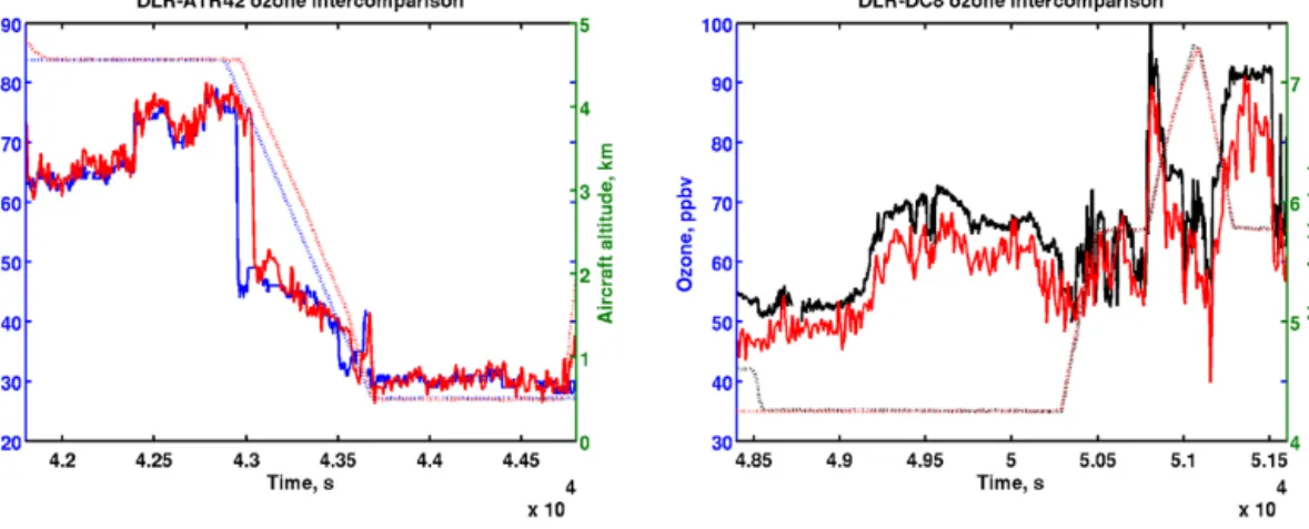
2008, the comparison of the ATR-42 and the DLR Falcon-20 ozone data at two altitude levels over Greenland (near 67◦N) shows an uncertainty better than 2 ppbv (Fig. 2). The NASA DC-8 (Weinheimer et al., 1994) O3 measurements
were made with a chemiluminescence technique, with the in-strument calibrated by additions of O3determined by UV
op-tical absorption at 254 nm. Uncertainties in the DC-8 O3data
are typically ±2 ppbv (±5 % of the signal). The NASA DC-8 flew mainly over Canadian forest fire regions in summer (Ja-cob et al., 2010). The comparison between the NASA DC-8 and the DLR Falcon-20 O3data during an aircraft
inter-comparison flight on 9 July over northern Greenland shows very good precision, but a 4 ppbv positive difference (Fig. 2). None of the Falcon-20 and NASA DC-8 data were corrected. The ALTO lidar was mounted in a zenith viewing mode making ozone vertical profiles above the aircraft, thus
limit-Figure 2. Intercomparison of O3measurements in ppbv (solid line and left vertical scale) during two wing tip-to-wing tip flights over
Greenland between the ATR-42 (blue) and the DLR Falcon-20 (red) on 14 July (left panel) and between the NASA-DC-8 (black) and the DLR Falcon-20 (red) on 9 July (right panel). The aircraft altitude changes are in km (dotted line and right vertical scale).
ing the number of O3data available at altitudes below 3 km.
The lidar measurement altitude range is of the order of 6 km above the aircraft flight level with a 300 m vertical resolution and a 10 km horizontal resolution (i.e., a 2 min integration time). The system is fully described in Ancellet and Ravetta (1998), and the instrument performances for different exam-ples of daytime airborne measurements are discussed in An-cellet and Ravetta (2003) (urban pollution in the boundary layer, ozone in the UTLS, and long-range transport in the free troposphere). Several comparisons with in situ measure-ments (ECC ozonesonde and airborne UV photometer) show no specific biases in clear air measurements. Measurements taken near clouds or thick aerosol layers are not included here since corrections of systematic errors related to aerosol inter-ference become very large (Papayannis et al., 1990). These represent 20 % of the lidar profiles recorded during the cam-paign.
The NASA-DC-8 Ozone DIAL system and configuration implemented during the campaign is described by Richter et al. (1997). The instrument provides simultaneous zenith and nadir profiles to cover the troposphere and lower strato-sphere. The O3measurement resolution is 300 m in the
ver-tical and approximately 70 km (3 min) in the horizontal for daytime measurements. On all field experiments, the air-borne DIAL O3measurements are compared with in situ O3
measurements made on the DC-8 during ascents, descents, and spirals, while comparisons to ozonesondes during coin-cident overflights were also conducted. In the troposphere, the DIAL O3measurements have been shown to be accurate
to better than 10 % or 2 ppb, whichever is larger (Browell et al., 1983, 1985). More recently, the precision of the DIAL O3measurements during the high-latitude SAGE-III Ozone
Loss and Validation Experiment in 2003 (SOLVE II) was found to be better than 5 % from near the surface to about 24 km and the accuracy was found to be better than 10 % in comparison with the Ny-Ålesund lidar, ozonesondes, and
in situ DC-8 measurements (Lait et al., 2004). DIAL and Microwave Limb Sounder (MLS) O3 measurements from
the Polar Aura Validation Experiment (PAVE) in 2005 were found to agree within 7 % across the 12–24 km altitude range (Froidevaux et al., 2008). Comparisons between DIAL and MLS were also examined in the upper troposphere and lower stratosphere (215–100 hPa region) from data obtained during the International Intercontinental Chemical Transport Exper-iment (INTEX-B) field experExper-iment, and these results show good agreement in the lower stratosphere, with decreasing performance of the MLS measurements into the troposphere (Livesey et al., 2008).
The ozonesonde monitoring was intensified in 2008 over North America in the framework of the ARCIONS initiative and the characteristics of the ozone measurements are fully described in Tarasick et al. (2010). Nearly daily soundings were made during the aircraft flight period at four stations over Canada between 53 and 63◦N, and at Summit,
Green-land, while weekly soundings were made at the high latitude stations Alert and Resolute.
The latitudinal cross sections of the ozone data set selected in this study are shown in Fig. 3 considering two domains to produce a bidimensional latitude–altitude plot over Canada (−160 to −70◦W) and Greenland (−70 to −20◦W). The horizontal distributions of the data set used for producing the latitude–altitude plots are shown in Fig. 1. For latitudes higher than 80◦N, the data comes from a limited number of observations: eight sondes from Alert and three DC-8 flights from 8 to 10 July. The locations of the ozonesonde stations are shown as red vertical bars in the latitudinal cross sections. In the troposphere at altitudes less than 8 km over Canada, lidar, in situ, and ozonesonde measurements contribute 67, 20, and 13 % of the ozone data set, respectively, while they correspond to 26, 69, and 5 %, respectively, over Greenland (see the number of observations using each technique in Ta-ble 3). The aircraft data (lidar and in situ) therefore strongly
Figure 3. Latitudinal cross section of the measured ozone mixing ratio in ppbv over Canada (left panel) and over Greenland (right panel). The red bars show the location of ozonesonde stations. Black regions with O3>160 ppbv correspond to the stratosphere.
Table 3. Mean, median, and standard deviation of the observed ozone mixing ratio in the different boxes shown in Figs. 7 and 9, except for the two boxes at latitudes > 80◦N, which have been merged in the last row of the table.
Zone Latitude Longitude Altitude O3mean O3median O3SD Number Number Number
N◦ range range km ppbv ppbv ppbv lidar in situ ECC 1 50–65◦N −132 to −70◦W 0–4 45.8 45.3 10.8 1046 422 243 2 65–80◦N −132 to −70◦W 0–4 42.3 40.9 11.4 401 27 28 3 50–63◦N −132 to −70◦W 4–8 69.4 68.0 18.8 1184 349 240 4 63–75◦N −132 to −70◦W 4–8 63.4 62.0 16.5 360 123 28 5 60–80◦N −70 to −20◦W 0–4 45.1 45.4 8.0 243 603 21 6 57–65◦N −70 to −20◦W 4–8 57.4 56.1 13.8 22 203 0 7 65–75◦N −70 to −20◦W 4–8 68.7 68.1 16.3 320 906 81 8 80–87◦N −132 to −20◦W 3–8 69.8 67.6 14.8 166 48 35
contribute to the high measurement density even though they correspond to a limited number of flying days, i.e., 18 days from 26 June to 18 July. In this work, ozone data are aver-aged hourly when they are in the same cell of a grid, with 0.5 × 0.5◦ and 1 km vertical resolution in order to avoid an
oversampling of similar air masses. Only hourly averages are considered in Table 3.
For both regions similar ozone vertical distributions were observed: low O3 mixing ratio ≤ 40 ppbv below 3 km and
high O3 concentrations typical of the UTLS in the altitude
range 8–11 km between 60 and 80◦N (i.e., red and dark region with O3 mixing ratio > 150 ppbv). The average O3
mixing ratio in the altitude range 4–8 km is of the order of 65 ppbv for both regions but the latitudinal O3gradients are
more visible over Greenland than over Canada. Two mid-tropospheric ozone branches are seen in the latitude band 65– 73 and 78–85◦N over Greenland, the former being tilted to the south at 70◦N and the latter to the north at 80◦N.
3 WRF-Chem model simulation 3.1 Model description
For this study we use the regional Weather Research Fore-casting model coupled with Chemistry (WRF-Chem) to study ozone during this period. WRF-Chem is a fully coupled, online meteorology and chemistry, and transport mesoscale model. It has been successfully used in Arctic-focused studies in the past (Thomas et al., 2013; Marelle et al., 2015) for both gas phase and aerosol analysis. Initial meteorological conditions and boundaries are from the Na-tional Center for Environmental Prediction (NCEP) Global Forecast System (GFS) with nudging applied to temperature, wind, and humidity every 6 h. The simulation uses the Noah Land Surface model scheme with four soil layers, the YSU (Yonsei University) planetary boundary layer (PBL) scheme (Hong et al., 2006), coupled with the MM5 similarity surface layer physics, the Morrison 2-moment (Morrison et al., 2009) microphysics scheme, and the Grell-3D ensemble (Grell and Dévényi, 2002) convective implicit parametrization. The ra-diation schemes are the Goddard (Chou and Suarez, 1994)
and rapid radiative transfer model (Mlawer et al., 1997) for shortwave and long wave radiation, respectively. Chemical boundary conditions were taken from the Model For Ozone and Related chemical Tracers, version 4 (Emmons et al., 2010). For gas phase chemical calculations the CBM–Z (Za-veri and Peters, 1999) chemical scheme is used and aerosols were calculated using the Model for Simulating Aerosol In-teractions and Chemistry (Zaveri et al., 2008). The model was run from 15 March to 1 August 2008 using a polar stereographic grid (100 × 100 km resolution) over a domain that covers most of the Northern Hemisphere, from about 28◦N. Vertically, 50 hybrid layers up to 50 hPa are used with approximately 10 levels in the first 2 km. The corre-sponding vertical resolution ranges from 100 m in the PBL to 500 m in the free troposphere. Anthropogenic emissions with a 0.5◦×0.5◦ spatial resolution were taken from the ECLIPSE (Evaluating the Climate and Air Quality Impacts of Short–Lived Pollutants) version 4.0 (Klimont et al., 2013). Wildfire emissions were taken from GFED 3.1 (van der Werf et al., 2010), while aircraft and shipping emissions were from the RCP 6.0 scenario (Lee et al., 2009 and Buhaug et al., 2009). Biogenic emissions were calculated online thanks to MEGAN (Model of Emissions of Gases and Aerosols from Nature) (Guenther et al., 2012).
Using observations from aircraft, surface stations, and satellites, atmospheric model simulations of O3 have been
evaluated as part of POLMIP, including WRF-Chem (Monks et al., 2015; AMAP, 2015). The model was run using differ-ent emissions and gas/aerosol schemes than in the POLMIP simulations, but the POLMIP results are still a good basis to choose WRF-Chem. While all models have deficiencies in reproducing trace gas concentration in the Arctic, WRF-Chem performs better than many models in re-producing tro-pospheric O3and CO, which are used here. Given the
advan-tages of also predicting stratosphere–troposphere exchange processes online for this study, WRF-Chem is a good model for interpreting these ozone climatologies constructed from measurements in summer 2008.
The WRF-Chem model does not explicitly calculate po-tential vorticity (PV). As a result, PV was calculated offline based on WRF meteorological fields: potential temperature, total mass density, geopotential height, and wind speed and direction. For each model grid cell, wind and temperature are interpolated from model vertical levels to the potential temperature in the center of the grid cell and the curl of the wind vector is calculated on the corresponding isentropic sur-faces using the original model grid (100 km × 100 km) and the full model vertical resolution, i.e., approximately 500 m in the free troposphere. Potential vorticity is expressed in potential vorticity units (PVu) using the definition 1 PVu = 10−6Kkg−1m−2s−1. The main uncertainty in the PV cal-culation is related to the representation of smaller scales (50 km) than the model resolution (e. g., narrow stratospheric streamers near the tropopause).
3.2 Model results interpolations
The measurements used in this study vary in temporal and spatial resolution (Sect. 2), where the model results are 3 hourly on a polar stereographic grid (described in Sect. 3). In order to avoid favoring data with the highest temporal resolution, the measured data were averaged to 1 min for all the in situ and lidar measurements. The ozonesondes are considered to be instantaneous at the time of the bal-loon release. A vertical resolution of 1 km is used for the lidars and ozonesondes. The measured data is then gridded to 0.5◦×0.5◦. If more than one measurement is available in the same grid box from the same campaign and instrument within an interval of one hour, then these are considered to be the same measurement, and a mean value is calculated.
The model grid cell, which is the most representative for the measurement’s location in space, is selected and a lin-ear interpolation in time is done to calculate 1 min incre-ments from the two modeled values separated by 3 h and surrounding the measurement time. In this way the two re-sulting data sets (modeled and measured) both have 1 min temporal resolution, and spatially only the vertical resolution is changed to set the altitude increment to 1 km. The model results, including PV, are also horizontally interpolated from 100 km resolution to match the new 0.5◦×0.5◦ horizontal data resolution. Each model grid cell is split into 100 mini-grid cells. Then each mini-mini-grid cell is assigned to the appro-priate 0.5◦×0.5◦ final grid cell before calculating the new model values.
4 Comparison of measured and modeled ozone
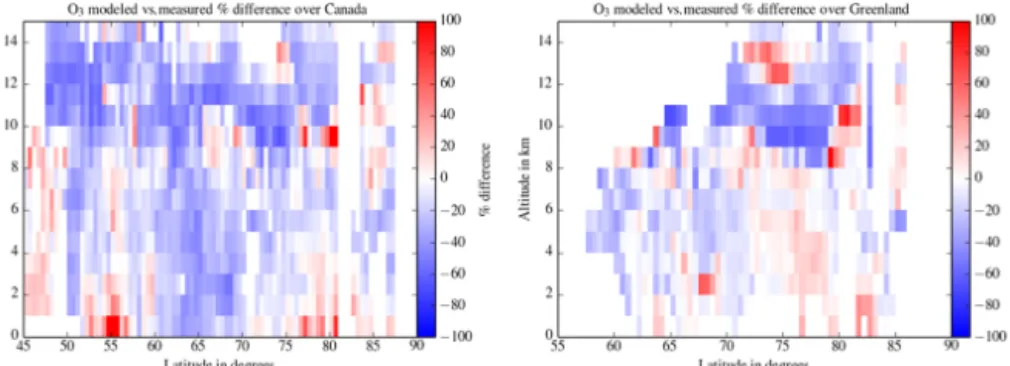
The WRF-Chem ozone mixing ratios corresponding to the times and locations of the June–July observations have been used to produce latitudinal cross sections comparable to the results shown in Fig. 3. The modeled O3latitudinal cross
sec-tions are shown for Canada and for Greenland in Fig. 4, while the corresponding relative differences between the model re-sults and the measurements are shown in Fig. 5. The altitude and latitude ozone variability of the model is comparable to the observations over both regions. The vertical structure, i.e., the transition between the low ozone values below 3 km and the higher ozone concentration in the free troposphere, and the UTLS ozone variability, are well reproduced. The latitudinal gradient of the ozone concentration in the 4–8 km altitude range over Greenland is also visible in the simulation results where the two mid-tropospheric ozone branches are also visible at 70 and 80◦N. This structure is slightly shifted in the modeled cross section explaining both positive and relative differences in the free troposphere over Greenland (Fig. 5). The agreement is less good for the latitudinal gra-dient over Canada where the low ozone values (< 50 ppbv) seen in the model at 65◦N in the mid-troposphere are not
Figure 4. Same as Fig. 3 but for the WRF-Chem model ozone mixing ratio corresponding to the measurement characteristics summarized in Tables 1 and 2.
Figure 5. Same as Figs. 3 and 4 for the ozone mixing ratio relative differences between the WRF-Chem model and the measurements.
seen in the observations, although the signs of the latitudinal gradients seem correct.
To quantify the observation–model agreement the scat-ter plot of modeled vs. measured ozone is also presented in Fig. 6 using a PV color scale to distinguish the tropospheric and stratospheric contributions. The measured vs. modeled O3correlation (red line in Fig. 6) is of the order of 0.9 in the
altitude range 0–15 km over both regions because the occur-rence of stratospheric ozone intrusions are very well repro-duced by WRF-Chem. The correlation is however between 0.5 and 0.7 in the troposphere only using observations with PV values less than 1 PVu (green line in Fig. 6). Considering that the ozone variability in the free troposphere is not very large (< 50 ppb), the spatial and temporal variability is still well reproduced by WRF-Chem even below the tropopause region. Even though the UTLS temporal variability is well reproduced by the model (Fig. 4), there is a significant under-estimation of ozone by a factor 1.5 in the WRF-Chem sim-ulation for the lowermost stratosphere (PV > 2 PVu) (Figs. 5 and 6). In the troposphere there is also a negative bias of the model data of the order of −6 to −15 ppbv with the largest differences over Canada (see Table 5). A fraction of this tro-pospheric underestimate by WRF-Chem is likely related to the O3underestimate in the lowermost stratosphere, causing
the stratospheric ozone source in the upper troposphere to be too small. The modeled O3underestimate in the lower
strato-sphere likely originates from the O3climatology used to
ini-tialize the model in the stratosphere. The other part of this 10-ppbv bias is due to an underestimate of the lightning NOx
contribution in the WRF-Chem simulation and/or an under-estimate of the vertical transport of continental emissions to the mid- and upper troposphere. Wespes et al. (2012) have shown that the lightning NOx source and vertical transport
of continental emissions both contribute to 15 % of the O3
concentration in the free troposphere at latitudes higher than 60◦N in summer. Despite these flaws, the WRF-Chem simu-lations are still very valuable because the spatial O3
variabil-ity compares rather well with the observations. The PV and CO distribution available from the WRF-Chem simulations will therefore be used to examine the respective roles of pho-tochemistry and STE in the observed ozone distribution in the following sections.
5 Latitudinal ozone distribution at high latitudes In this section, we investigate the mean latitudinal and verti-cal ozone gradient in the troposphere using the POLARCAT observations. To quantify these gradients, the O3 cross
sec-. Figure 6. Scatter plot of WRF-Chem modeled vs. measured O3
mixing ratio in ppbv for Canada (top panel) and Greenland (bottom panel) domains. The black lines are the one-to-one line and the PV color scale distinguishes stratospheric (red and white dots) and tro-pospheric data (blue and green dots). The regression line parameters and the Pearson correlation coefficient with its p value are colored in red and green for the PV range 0–4 and 0–1 PVu, respectively.
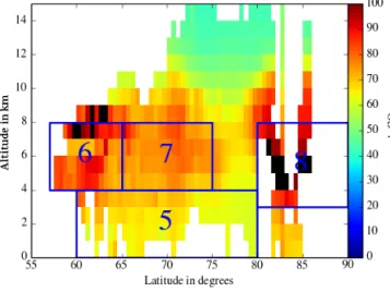
tions plotted in Fig. 3 have been divided into several regions using the model CO latitudinal cross sections. The vertical boundaries are defined according to the mean ozone vertical profile in the troposphere, i.e., the depth of the low ozone val-ues layer in the lower troposphere and the downward extent of the tropopause region. The variability of the CO distri-bution is only taken from the model, since CO data is not available for many of the ozone observations (ozonesonde and lidar profiles).
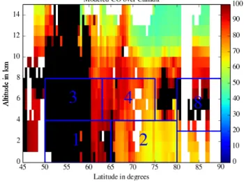
Figure 7. Latitudinal cross section of the modeled CO mixing ratio in ppbv over Canada for the measurement of spatiotemporal distri-bution from the June–July 2008 WRF-Chem simulation. The blue boxes correspond to the regions where data are averaged for dis-cussing vertical and latitudinal gradients in Table 4.
5.1 Measurements over Canada
For the data taken over Canada, five regions were consid-ered to calculate the mean O3latitudinal gradient. They
cor-respond to the blue boxes with the labels 1, 2, 3, 4, and 8 shown in the CO latitudinal distribution plotted in Fig. 7. The different zones have similar regional extent in order to make them comparable. Two are below 4 km in the altitude range where the lowest ozone values were recorded for lati-tudes > 60◦N. The boundary between these two boxes is set
according to the strong CO latitudinal difference, due to the biomass burning emissions south of 65◦N and lack of local emissions of ozone precursors in the region between 65 and 80◦N. In the altitude range 4–8 km, which corresponds to the largest tropospheric ozone values, two other regions were de-fined. The latitude boundary at 63◦N is again prescribed ac-cording to the latitude where CO and O3concentrations are
simultaneously decreasing. The last box corresponds to the tropospheric observations at high latitudes (> 80◦N) where CO concentrations are increasing, especially in the altitude range 3–8 km. These ozone observations were mainly made in northeastern Canada by the DC-8 aircraft. The CO distri-bution derived from the WRF-Chem simulation is consistent with the analysis of CO observations by Bian et al. (2013), who show the major influence of boreal and Asian emissions on the ARCTAS-B CO observations.
The mean and median measured O3mixing ratios for the
different boxes are shown in Table 3, along with the number of observations from the different measurement techniques (lidar, in situ, and sondes). The mean and median O3and CO
mixing ratios from the model are also reported in Table 4 and the statistics relevant to the model evaluation are reported in Table 5. The −10 to −15 ppbv differences between the
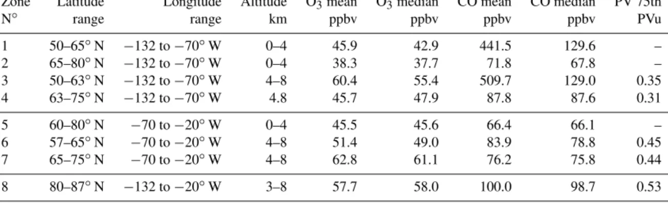
Table 4. Same as Table 3 for the WRF-Chem model O3, CO mixing ratio, and PV 75th percentile.
Zone Latitude Longitude Altitude O3mean O3median CO mean CO median PV 75th
N◦ range range km ppbv ppbv ppbv ppbv PVu
1 50–65◦N −132 to −70◦W 0–4 45.9 42.9 441.5 129.6 – 2 65–80◦N −132 to −70◦W 0–4 38.3 37.7 71.8 67.8 – 3 50–63◦N −132 to −70◦W 4–8 60.4 55.4 509.7 129.0 0.35 4 63–75◦N −132 to −70◦W 4.8 45.7 47.9 87.8 87.6 0.31 5 60–80◦N −70 to −20◦W 0–4 45.5 45.6 66.4 66.1 – 6 57–65◦N −70 to −20◦W 4–8 51.4 49.0 83.9 78.8 0.45 7 65–75◦N −70 to −20◦W 4–8 62.8 61.1 76.2 75.8 0.44 8 80–87◦N −132 to −20◦W 3–8 57.7 58.0 100.0 98.7 0.53
Table 5. Metrics of the WRF-Chem O3simulation performance for the regions reported in Table 4: mean bias, root mean square error
(RMSE), normalized mean bias.
Zone Latitude Longitude Altitude Mean bias RMSE Normalized N◦ range range km ppbv ppbv mean bias, % 1 50–65◦N −132 to −70◦W 0–4 0.1 24.0 0.3 2 65–80◦N −132 to −70◦W 0–4 −4 10.3 −9.5 3 50–63◦N −132 to −70◦W 4–8 −9 24.9 −12.9 4 63–75◦N −132 to −70◦W 4.8 −15 21.9 −28.0 5 60–80◦N −70 to −20◦W 0–4 0.4 7.5 0.8 6 57–65◦N −70 to −20◦W 4–8 −6 15.3 −10.6 7 65–75◦N −70 to −20◦W 4–8 −6 17.1 −8.6 8 80–87◦N −132 to −20◦W 3–8 −13 18.0 −17.2
model and measured ozone in zones 3, 4, and 8 above 4 km are consistent with the bias of the model in the troposphere over Canada discussed in the previous section. This bias is small (0 to −4 ppbv) in the lower troposphere, showing that the emissions used in the model simulation are good enough to calculate the O3photochemical production.
The negative latitudinal gradient of ozone between zones 3 and 4 (1O3= −6 ppbv for the measurements and 1O3≈
−8 ppbv for the model), and to a lesser extent between zones 1 and 2 (1O3= −4 ppbv for the measurements and 1O3=
−5 ppbv for the model), are correlated with a significant negative latitudinal CO gradient. Here we compare median rather than mean values as the latter are biased by a few very high values (see below). For latitudes lower than 65◦N there
is a strong standard deviation because some of the measure-ments were taken very close to fresh biomass burning sources (forest fires). Sampling of the biomass burning sources dur-ing ARCTAS by the DC-8 aircraft between 50 and 63◦N has already been discussed in several papers (Singh et al., 2010; Alvarado et al., 2010; Thomas et al., 2013). In the mid-troposphere the CO enhancement in zone 3, where the largest O3 mixing ratio (70 ppbv) is recorded, is 130 ppbv,
well above the CO tropospheric baseline of 60 ppbv (the strong difference between the mean and the median
corre-sponds to the sampling of one biomass burning plume with CO > 500 ppbv, which biases the mean). Zone 8 data in Ta-bles 3 and 4 combines the aircraft sampling over both Canada and Greenland for the high latitude boxes (> 80◦N) because they characterize regions with similar O3 and CO
distribu-tions. The O3 mean for zone 8 (70 ppbv) is similar to the
one found in zone 3, while CO is increasing again at high latitudes (40 ppbv above the CO tropospheric baseline of 60 ppbv).
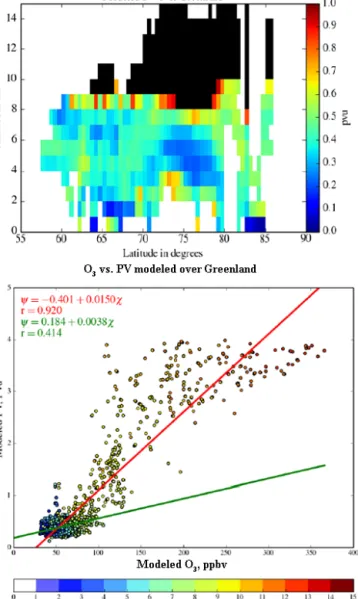
The average PV latitudinal cross section is also calculated for the ozone data set as it is a good tracer of the latitudinal variability of the stratospheric O3source (Fig. 8). Although
frequent stratospheric air mass intrusions are seen in the 8– 10 km altitude range at latitudes higher than 55◦N, the role
of the stratospheric source is not clearly visible in the aver-age PV values in the free troposphere. Mean PV values larger than 0.5 PVu are only seen for latitudes higher than 75◦N in the 3–6 km altitude range (the large PV values at altitudes below 2 km should not be considered as they are related to the low level cyclonic circulation due the orographic circu-lation around the Greenland ice cap). This suggests that the latitudinal ozone gradients between zones 3 and 4 are not related to the latitudinal distribution of stratospheric intru-sions. However, O3mixing ratios larger than 70 ppbv (Fig. 3)
Figure 8. Latitudinal cross section of the average PV profiles over Canada for the summer measurement distribution using the WRF-Chem simulation (top panel). Scatterplot of modeled O3 in ppbv
vs. PV in PVu using an altitude color coded scale (bottom panel). Stratospheric data points with PV > 4 PVu are not included. The regression line parameters and the Pearson correlation coefficient with its p value are also given for the PV range 0–4 PVu (red) and 0–1 PVu (green).
are correlated with the descending high PV tongue at lati-tudes between 77 and 87◦N (Fig. 8). Because the analysis of
the ozone spatial distribution shows contrasting behavior of the ozone–PV relationship, it is also necessary to look at the PV vs. O3mixing ratio scatter plot. When only tropospheric
ozone data are considered (PV < 1 PVu), there is a poor Pear-son correlation (r < 0.3) between ozone and PV, implying that stratospheric intrusions are not the only source of high tropospheric ozone values (Fig. 8). Indeed one can see that a significant number of high tropospheric ozone mixing ratios
. Figure 9. Same as Fig. 7 but for the Greenland region.
(> 70 ppbv) are related to PV less than 1 PVu when using the altitude color scale to separate the UTLS (8–10 km) and tro-pospheric data. The difference in the slopes of the regression line, when including or not including the PV values larger than 1 PVu (red vs. green lines in Fig. 8), is also larger than similar variation observed at mid-latitudes in Europe where the O3 to PV ratio decreases from 30 to 150 ppbv / PVu
(Ravetta et al., 1999). This suggests that the ozone variabil-ity during summer 2008 is not driven by the variabilvariabil-ity of stratospheric air mixed into the free troposphere, but mainly related to emissions and photochemistry over Canada. 5.2 Measurements over Greenland
The same procedure was applied to the latitudinal distribu-tion over Greenland. The regions considered for the latitu-dinal gradient analysis are slightly different because the CO latitudinal cross sections and the ozone vertical structure are different. The selected regions are shown by the blue boxes in Fig. 9. Only one zone is chosen between 60 and 80◦N for the altitude range below 4 km, where there are the low-est tropospheric O3and CO concentrations values. The CO
latitudinal gradient is indeed very weak in the lower tropo-sphere between 60 and 80◦N (< 5 ppbv). However, as over Canada, two boxes are chosen in the altitude range 4–8 km because of their differences in terms of CO and O3
concen-trations. An additional box corresponds to the tropospheric observations at high latitudes (> 80◦N) where the CO
con-centrations are also higher, especially in the altitude range 3–8 km. This is related to the observations mainly made in northwestern Greenland by the DC-8 aircraft.
Table 5 shows that there is no O3 underestimate by the
model in the lower troposphere and the model bias above 4 km is of the order of −6 ppbv. This suggests that the model performance over Greenland, away from the conti-nental sources, is better than over Canada. The remaining
Figure 10. Same as Fig. 8 but for the Greenland region.
−6 ppbv bias can be easily explained by the stratospheric O3
climatology having too low values, while lightning is known to be less important over Greenland (Cecil et al., 2014; Chris-tian et al., 2003). The CO concentration in the lower tro-posphere (zone 5 of Table 3) is close to the tropospheric baseline, while O3 is not markedly different from the
val-ues seen over Canada. The positive latitudinal O3 gradient
between zones 6 and 7 in the mid-troposphere above 4 km (1O3=12 ppbv) is two times larger than the latitudinal
gra-dient over Canada, but the overall O3mid-tropospheric
con-centration over Greenland is similar to its counterpart over Canada (62 vs. 65 ppbv). The corresponding negative CO lat-itudinal gradient between zone 6 and 7 is weak (difference of 8 ppbv), but it is anticorrelated with the ozone gradient. The CO excess above baseline is only 20 ppbv in zone 6, where CO is maximum. The anticorrelation between the O3
and CO latitudinal gradient may indicate more occurrences
of stratospheric ozone intrusion in zone 7 at latitudes higher than 65◦N during the POLARCAT period. If the lower CO
were due to upwelling of pristine air from the Arctic lower troposphere, it would be accompanied by smaller O3
concen-trations according to Fig. 3.
Looking at the average PV distribution extracted from the WRF-Chem simulation (Fig. 10), frequent stratospheric air mass intrusions are seen in the altitude range 8–10 km, es-pecially at 75◦N (PV > 1 PVu). PV values are also larger in the mid-troposphere over Greenland than over Canada (75th PV percentile is 0.45 PVu over Greenland but 0.3 PVu over Canada). The PV vs. O3mixing ratio scatter plot also shows
a higher Pearson correlation (r > 0.4) between ozone and stratospheric intrusion than over Canada (Fig. 10). Compared to the results obtained over Canada, the difference between the O3-to-PV ratio, including PV values larger than 1, and
that excluding them (red vs. green regression line) is smaller (200 ppbv / PVu instead of 400 ppbv / PVu for Canada). This is consistent with a larger fraction of ozone from the UTLS over Greenland. However, there is not a significant latitudi-nal PV gradient in the mid-troposphere between zones 6 and 7 where a positive 12 ppbv ozone latitudinal gradient is de-tected. At high latitudes above 80◦N, the PV and CO latitu-dinal distribution in the troposphere is almost identical to the latitudinal cross section over Canada (Fig. 8), which supports merging data in a single zone 8 for the statistics reported in Tables 3 and 4.
5.3 Discussion
This section aims to discuss the latitudinal ozone distribu-tion above Greenland and Canada using (i) existing studies of the role of biomass burning, anthropogenic emissions, and STE on high latitude tropospheric ozone, (ii) satellite obser-vations of biomass burning locations and associated plumes during summer 2008, and (iii) back trajectory analysis of the air masses where observations were made.
In the lower troposphere (0–4 km), the fact that ozone is lower than 50 ppbv everywhere (except close to the fires southwest of Hudson Bay) is expected, considering a near zero net ozone photochemical production (+0.3 ppbv day−1 near the surface and −0.3 ppbv day−1 in the lowermost free troposphere) and a weak influence of STE below 5 km in Northern Canada (Walker et al., 2012; Mauzerall et al., 1996).
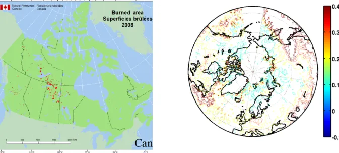
In the free troposphere above 4 km, a negative CO lati-tudinal gradient in the latitude range 50–75◦N is seen over
both Greenland and Canada. The large CO latitudinal gra-dient over Canada can only be explained when considering the biomass burning plume at the continental scale which is superimposed onto the anthropogenic emissions south of 50◦N. The position of the biomass burning plume is shown by the MODIS monthly mean aerosol optical depth, together with the Canadian Forest Service (CFS) fire counts (Fig. 11). Maxima of aerosol optical depth are seen both southwest
Figure 11. Map of the Canadian Forest Service fire counts in red for summer 2008 (left) and MODIS aerosol optical depth at 0.55 µm from 15 June to 15 July 2008 (right).
Figure 12. Map of the air mass daily positions using 4 days FLEXTRA trajectories, which correspond to the observations in zones 3 and 4 over Canada (top row) and in zones 6 and 7 over Greenland (bottom row). Black crosses show the measurement positions and the color scale is the air mass altitude in km. The fraction is the relative number of trajectory positions reaching the tropopause (PV = 1.5 PVu).
of Hudson Bay and over the Atlantic Ocean in the latitude band 50 to 60◦N. The ozone latitudinal gradient is also neg-ative and correlated with CO over Canada, which can be explained by ozone photochemical production in the Cana-dian biomass burning plumes. Thomas et al. (2013) showed
a 3 ppbv ozone increase downwind of biomass burning emis-sions and an enhancement ratio 1O3/1CO ranging from 0.1
near the fires to 0.5 downwind from the fires. This is con-sistent with a 1O3 of 6–8 ppbv between zone 3 and 4 over
Figure 13. Same as Fig. 12 for the observations at latitudes > 80◦N in zone 8.
is found in the model simulation. The contribution of other emission sources can be also estimated using 4 day back-ward trajectories calculated with the FLEXTRA model and T213/L91 ECMWF analysis (Fig. 12). According to the up-per panels of Fig. 12, long-range transport into zones 3 and 4 over Canada shows similar patterns with 75 % of the air masses coming from North American mid-latitudes, i.e., the area between −60 and −150◦W and 50 and 70◦N. Regional variability of STE also has a weak influence during this pe-riod, considering the weak dependency of O3with PV over
Canada. Local emissions from biomass burning are the most reasonable explanation for the ozone latitudinal gradient be-tween 50 and 75◦N.
Over southern Greenland the effect of ozone photochem-ical production related to fire plumes and the North Ameri-can anthropogenic emissions appears to be less than 4 ppbv, considering the weak CO gradient between zones 6 and 7 (≈ −8 ppbv). The negative O3gradient due to increased
pho-tochemical production in zone 6 can then be easily counter-balanced by another source in zone 7 to explain the posi-tive latitudinal O3gradient over Greenland. The STE ozone
source is a likely contributor, as suggested by the better cor-relation between O3and PV over Greenland than Canada and
larger PV over Greenland. Frequent tropopause polar vor-tices developing over Baffin Bay and Davis Strait still oc-cur during the summer period because of the important role of radiation to maintain and intensify the upper troposphere cyclonic activity during the summer (Cavallo and Hakim,
2010). However, in the absence of a clear PV latitudinal gra-dient between 55 and 75◦N in the model, simulation cannot explain the significant +12 ppbv ozone latitudinal gradient. Therefore, while STE certainly contributes to the ozone bud-get over both southern and northern Greenland, it does not explain the largest O3values found in zone 7. Looking at the
long-range transport plot for zones 6 and 7 (lower panels of Fig. 12), the fraction of air masses coming from the North American mid-latitude area are now 34 and 18 %, respec-tively. Multiple mid-latitude sources, including North Amer-ica, Europe, and even Asia, are also related to ozone obser-vations in zone 7, and may explain the differences in ozone production efficiency between zone 6 and zone 7. Wespes et al. (2012) concluded using the Model MOZART-4 that anthropogenic pollution from Europe dominates O3
concen-trations in summer 2008 in the Arctic, while Roiger et al. (2011) shows, using aircraft measurements, that Asian an-thropogenic pollution can be mixed with stratospheric air masses over Greenland in the 75–80◦latitude band.
For the free troposphere at high latitudes above 80◦N,
the STE contribution is maximum in this region for the 4– 8 km altitude range according to the average PV distribu-tion shown in Fig. 8 or Fig. 10. The 75th percentile of the PV distribution is also > 0.5 PVu in zone 8, while it is 0.3 PVu at latitudes lower than 75◦over Canada and 0.4 PVu over Greenland. Zängl and Hoinka (2001) discussed the hor-izontal gradient of the tropopause height over the Arctic using ECMWF analysis and radiosondes. The region with
the largest horizontal gradient is displaced to the north near 80◦N in July over North America, while vertical tilting of
the isentropic surfaces remains small. These conditions are favorable for isentropic motion across the tropopause with more efficient STE. However CO also increases at high lat-itude because of transport from Asian and northern Siberian pollution sources, according to the air mass transport path-way for zone 8 (Fig. 13). Such a mixture of stratospheric O3
and Asian pollution has already been suggested by Roiger et al. (2011) to explain the ozone concentrations observed at very high latitudes in the Arctic. Our study, using more ozone measurements, leads to the same conclusions.
6 Conclusions
The purpose of this work is to provide a complete pic-ture of Arctic ozone using measurements available during the summer 2008 POLARCAT campaigns over Canada and Greenland, where three aircraft were deployed and seven ozonesonde stations intensified their ozone vertical profil-ing. This is the first case of such complete temporal and ge-ographical coverage. We take advantage of the large number of airborne lidar profiles (representing 67 % of the O3
surements over Canada and 26 % over Greenland). The mea-sured ozone climatology established in this paper can also be used for future model evaluation at high latitudes. For ex-ample, in our work, while good correspondence of the mea-sured O3 vertical and latitudinal distribution is found with
model results from WRF-Chem, a negative O3bias of −6 to
−15 ppbv between the model and the observations is found in the free troposphere over 4 km, especially over Canada. This deficiency is partly related to the WRF-Chem model strato-spheric ozone initialization.
The WRF-Chem model simulation is also used to dis-cuss the relative influence of tropospheric ozone sources at high latitude in summer. Ozone average concentrations are of the order of 65 ppbv at altitudes above 4 km both over Canada and Greenland, while they are less than 50 ppbv in the lower troposphere. For Canada, the analysis of the mod-eled CO distribution and the weak correlation (< 30 %) of O3 and PV suggest that stratosphere–troposphere exchange
(STE) is not the major contribution to tropospheric ozone at latitudes less than 70◦N, where transport of North American biomass burning (BB) emissions took place during the 2008 summer. Conversely, significant STE is found over Green-land according to the better O3vs. PV correlation (> 40 %)
and the higher value of the 75th PV percentile. This is related to the persistence of cyclonic activity over Baffin Bay during the summer.
A weak negative latitudinal summer ozone gradient of −6 to −8 ppbv is found over Canada in the mid-troposphere be-tween 4 and 8 km because the O3photochemical production
from BB emissions mainly takes place at latitudes less than 65◦N, while STE plays a larger role at latitudes higher than 70◦N. A positive ozone latitudinal gradient of 12 ppbv is ob-served in the same altitude range over Greenland not because of an increasing latitudinal influence of STE, but because of different long-range transport from multiple mid-latitude sources (North America, Europe, and even Asia for latitudes higher than 77◦N).
For the Arctic latitudes (> 80◦N), free tropospheric O3
concentrations are related to a mixture of stratospheric O3
transport across the tropopause and Asian pollution, as al-ready suggested by Roiger et al. (2011) using a case study of aircraft observations in the Arctic. Our study, which uses more ozone measurements, leads to the same conclusions.
7 Data availability
The CNRS ATR-42 aircraft ozone lidar observations can be downloaded from ftp://[email protected]. fr/Kanger/LidarO3/ (Ancellet, 2009a) and the the meta-data file is called “ReadmeO3lidarmeta-data”. The CNRS ATR-42 ozone situ measurements from the MOZART in-strument are deposited on ftp://ftp.aero.jussieu.fr/Kanger/ Data_ATR/ (Ancellet, 2009b) and the meta-data file is called “Readme_MOZART.txt”. Requested password is “kanger” to access the CNRS data. The data from the NASA DC-8 aircraft have been downloaded from the NASA archive website, using a direct Link to the DIAL data archive (http://www-air.larc.nasa.gov/cgi-bin/ ArcView/arctas#HAIR.JOHN/, Hair, 2008) and to the ozone in-situ measurements (http://www-air.larc.nasa.gov/cgi-bin/ ArcView/arctas#WEINHEIMER.ANDREW/, ). No pass-words are required as this is open and public access. The POLARCAT ozone data for DLR Falcon-20 is available from the HALO/Falcon database (https://halo-db.pa.op.dlr. de/). ECC ozonesonde data have been downloaded from the ARCIONS web site ftp://es-ee.tor.ec.gc.ca/pub/ftpdt/ ARC-IONSData/summer/ICARTT/ (Tarasick, 2008) and the WOUDC web site (http://woudc.org/data/explore.php?lang= en). Data files from the WRF model simulation are too big to be publicly available but could be obtained from LATMOS. Air mass trajectories are calculated with ECMWF meteoro-logical analysis downloaded from ECMWF MARS data base which is not publicly available.
Acknowledgements. We are very grateful to the support of the Meteo France/CNRS/CNES UMS SAFIRE for the ATR-42 aircraft deployment over Greenland. This work was supported by funding from ANR and LEFE INSU/CNRS (CLIMSLIP project) and from the ICE-ARC programme from the European Union 7th Framework Programme, grant number 603887. The FLEXTRA team (A. Stohl, and co-workers) is acknowledged for providing and supporting the FLEXTRA code. NASA and DLR are acknowledged for their support of the deployment of the DC-8 and Falcon-20 aircraft. WOUDC and the NASA MODIS team are acknowledged for providing the ozonesonde data and the MODIS data, respectively. Edited by: E. Harris
Reviewed by: two anonymous referees
References
Abbatt, J. P. D., Thomas, J. L., Abrahamsson, K., Boxe, C., Gran-fors, A., Jones, A. E., King, M. D., Saiz-Lopez, A., Shep-son, P. B., Sodeau, J., Toohey, D. W., Toubin, C., von Glasow, R., Wren, S. N., and Yang, X.: Halogen activation via interac-tions with environmental ice and snow in the polar lower tropo-sphere and other regions, Atmos. Chem. Phys., 12, 6237–6271, doi:10.5194/acp-12-6237-2012, 2012.
Alvarado, M. J., Logan, J. A., Mao, J., Apel, E., Riemer, D., Blake, D., Cohen, R. C., Min, K.-E., Perring, A. E., Browne, E. C., Wooldridge, P. J., Diskin, G. S., Sachse, G. W., Fuelberg, H., Sessions, W. R., Harrigan, D. L., Huey, G., Liao, J., Case-Hanks, A., Jimenez, J. L., Cubison, M. J., Vay, S. A., Weinheimer, A. J., Knapp, D. J., Montzka, D. D., Flocke, F. M., Pollack, I. B., Wennberg, P. O., Kurten, A., Crounse, J., Clair, J. M. St., Wisthaler, A., Mikoviny, T., Yantosca, R. M., Carouge, C. C., and Le Sager, P.: Nitrogen oxides and PAN in plumes from boreal fires during ARCTAS-B and their impact on ozone: an integrated analysis of aircraft and satellite observations, Atmos. Chem. Phys., 10, 9739–9760, doi:10.5194/acp-10-9739-2010, 2010. AMAP: Assessment 2015: Black carbon and ozone as
Arc-tic climate forcers. Arctic Monitoring and Assessment Programme (AMAP), Arctic Monitoring and Assessment Programme (AMAP), Oslo, Norway, 1–116, available at: http://www.amap.no/documents/doc/, 2015.
Ancellet, G.: CNRS ATR-42 aircraft ozone lidar observations, LAT-MOS/IPSL, UPMC Univ. Paris 06 Sorbonne Université, UVSQ, CNRS, Paris, France, available: ftp://[email protected]. fr/Kanger/LidarO3/, 2009a.
Ancellet, G.: CNRS ATR-42 ozone in-situ measurements, LAT-MOS/IPSL, UPMC Univ. Paris 06 Sorbonne Universités, UVSQ, CNRS, Paris, France, avilable at: ftp://ftp.aero.jussieu.fr/Kanger/ Data_ATR/, 2009b.
Ancellet, G. and Ravetta, F.: Compact airborne lidar for tropo-spheric ozone: description and field measurements, Appl. Opt., 37, 5509–5521, doi:10.1364/AO.37.005509, 1998.
Ancellet, G. and Ravetta, F.: On the usefulness of an air-borne lidar for O3 layer analysis in the free troposphere and the planetary boundary layer, J. Environ. Monit., 5, 47–56, doi:10.1039/B205727A, 2003.
Bian, H., Colarco, P. R., Chin, M., Chen, G., Rodriguez, J. M., Liang, Q., Blake, D., Chu, D. A., da Silva, A., Darmenov, A.
S., Diskin, G., Fuelberg, H. E., Huey, G., Kondo, Y., Nielsen, J. E., Pan, X., and Wisthaler, A.: Source attributions of pollution to the Western Arctic during the NASA ARCTAS field campaign, Atmos. Chem. Phys., 13, 4707–4721, doi:10.5194/acp-13-4707-2013, 2013.
Browell, E., Carter, A., Shipley, S., Allen, R., Butler, C., Mayo, M., Siviter Jr., J., and Hall, W.: NASA multipurpose airborne DIAL system and measurements of ozone and aerosol profiles, Appl. Opt., 22, 522–534, doi:10.1364/AO.22.000522, 1983.
Browell, E., Ismail, S., and Shipley, S.: Ultraviolet DIAL measurements of O3 profiles in regions of spatially
inhomogeneous aerosols, Appl. Opt., 24, 2827–2836, doi:10.1364/AO.24.002827, 1985.
Browell, E. V., Hair, J. W., Butler, C. F., Grant, W. B., DeYoung, R. J., Fenn, M. A., Brackett, V. G., Clayton, M. B., Brasseur, L. A., Harper, D. B., Ridley, B. A., Klonecki, A. A., Hess, P. G., Emmons, L. K., Tie, X., Atlas, E. L., Cantrell, C. A., Wimmers, A. J., Blake, D. R., Coffey, M. T., Hannigan, J. W., Dibb, J. E., Talbot, R. W., Flocke, F., Weinheimer, A. J., Fried, A., Wert, B., Snow, J. A., and Lefer, B. L.: Ozone, aerosol, potential vorticity, and trace gas trends observed at high-latitudes over North Amer-ica from February to May 2000, J. Geophys. Res.-Atmos., 108, 8369, doi:10.1029/2001JD001390, 2003.
Buhaug, O., Corbett, J., Endresen, O., Eyring, V., Faber, J., Hanayama, S., Lee, D. S., Lee, D., Lindstad, H., Markowska, A., Mjelde, A., Nelissen, D., Nilsen, J., Palsson, C., Winebrake, J., Wu, W., and Yoshida, K.: Second IMO GHG study 2009, Interna-tional Maritime Organization (IMO) London, UK, Tech. Report, 2009.
Cavallo, S. M. and Hakim, G. J.: Composite Structure of Tropopause Polar Cyclones, Mon. Weather Rev., 138, 3840– 3857, doi:10.1175/2010MWR3371.1, 2010.
Cecil, D. J., Buechler, D. E., and Blakeslee, R. J.: Grid-ded lightning climatology from TRMM-LIS and OTD: Dataset description, Atmos. Res., 135–136, 404–414, doi:10.1016/j.atmosres.2012.06.028, 2014.
Chou, M.-D. and Suarez, M. J.: An efficient thermal infrared ra-diation parameterization for use in general circulation mod-els, NASA Tech. Memorandum 104606-Vol 3, NASA, Goddard Space Flight Center, Greenbelt, MD, 1994.
Christian, H. J., Blakeslee, R. J., Boccippio, D. J., Boeck, W. L., Buechler, D. E., Driscoll, K. T., Goodman, S. J., Hall, J. M., Koshak, W. J., Mach, D. M., and Stewart, M. F.: Global fre-quency and distribution of lightning as observed from space by the Optical Transient Detector, J. Geophys. Res.-Atmos., 108, 4005, doi:10.1029/2002JD002347, 2003.
Cooper, O. R., Parrish, D. D., Stohl, A., Trainer, M., Nedelec, P., Thouret, V., Cammas, J. P., Oltmans, S. J., Johnson, B. J., Tara-sick, D., Leblanc, T., McDermid, I. S., Jaffe, D., Gao, R., Stith, J., Ryerson, T., Aikin, K., Campos, T., Weinheimer, A., and Av-ery, M. A.: Increasing springtime ozone mixing ratios in the free troposphere over western North America, Nature, 463, 344–348, doi:10.1038/nature08708, 2010.
Crutzen, P., Lawrence, M., and Pöschl, U.: On the background photochemistry of tropospheric ozone, Tellus B, 51, 123–146, doi:10.3402/tellusb.v51i1.16264, 1999.
Dupont, R., Pierce, B., Worden, J., Hair, J., Fenn, M., Hamer, P., Natarajan, M., Schaack, T., Lenzen, A., Apel, E., Dibb, J., Diskin, G., Huey, G., Weinheimer, A., Kondo, Y., and Knapp,
D.: Attribution and evolution of ozone from Asian wild fires us-ing satellite and aircraft measurements durus-ing the ARCTAS cam-paign, Atmos. Chem. Phys., 12, 169–188, doi:10.5194/acp-12-169-2012, 2012.
Emmons, L. K., Walters, S., Hess, P. G., Lamarque, J.-F., Pfister, G. G., Fillmore, D., Granier, C., Guenther, A., Kinnison, D., Laepple, T., Orlando, J., Tie, X., Tyndall, G., Wiedinmyer, C., Baughcum, S. L., and Kloster, S.: Description and evaluation of the Model for Ozone and Related chemical Tracers, version 4 (MOZART-4), Geosci. Model Dev., 3, 43–67, doi:10.5194/gmd-3-43-2010, 2010.
Fast, J. D., Gustafson, W. I., Easter, R. C., Zaveri, R. A., Barnard, J. C., Chapman, E. G., Grell, G. A., and Peckham, S. E.: Evolution of ozone, particulates, and aerosol direct ra-diative forcing in the vicinity of Houston using a fully coupled meteorology-chemistry-aerosol model, J. Geophys. Res.-Atmos., 111, D21305, doi:10.1029/2005JD006721, 2006.
Froidevaux, L., Jiang, Y. B., Lambert, A., Livesey, N. J., Read, W. G., Waters, J. W., Browell, E. V., Hair, J. W., Avery, M. A., McGee, T. J., Twigg, L. W., Sumnicht, G. K., Jucks, K. W., Margitan, J. J., Sen, B., Stachnik, R. A., Toon, G. C., Bernath, P. F., Boone, C. D., Walker, K. A., Filipiak, M. J., Harwood, R. S., Fuller, R. A., Manney, G. L., Schwartz, M. J., Daffer, W. H., Drouin, B. J., Cofield, R. E., Cuddy, D. T., Jarnot, R. F., Knosp, B. W., Perun, V. S., Snyder, W. V., Stek, P. C., Thurstans, R. P., and Wagner, P. A.: Validation of Aura Microwave Limb Sounder stratospheric ozone measurements, J. Geophys. Res.-Atmos., 113, D5S20, doi:10.1029/2007JD008771, 2008. Granier, C., Niemeier, U., Jungclaus, J. H., Emmons, L., Hess, P.,
Lamarque, J.-F., Walters, S., and Brasseur, G. P.: Ozone pollution from future ship traffic in the Arctic northern passages, Geophys. Res. Lett., 33, L13807, doi:10.1029/2006GL026180, 2006. Grell, G. and Dévényi, D.: A generalized approach to
pa-rameterizing convection combining ensemble and data assimilation techniques, Geophys. Res. Lett., 29, 1693, doi:10.1029/2002GL015311, 2002.
Grell, G. A., Peckham, S. E., Schmitz, R., McKeen, S. A., Frost, G., Skamarock, W. C., and Eder, B.: Fully coupled online chem-istry within the WRF model, Atmos. Environ., 39, 6957–6975, doi:10.1016/j.atmosenv.2005.04.027, 2005.
Guenther, A. B., Jiang, X., Heald, C. L., Sakulyanontvittaya, T., Duhl, T., Emmons, L. K., and Wang, X.: The Model of Emissions of Gases and Aerosols from Nature version 2.1 (MEGAN2.1): an extended and updated framework for modeling biogenic emis-sions, Geosci. Model Dev., 5, 1471–1492, doi:10.5194/gmd-5-1471-2012, 2012.
Hair, F.: NASA DC-8 aircraft data, DIAL data archive, NASA Langley Reasearch Center, Hampton, VA, USA, available at: http://www-air.larc.nasa.gov/cgi-bin/ArcView/arctas#HAIR. JOHN/, 2008.
Hess, P. G. and Zbinden, R.: Stratospheric impact on tropospheric ozone variability and trends: 1990–2009, Atmos. Chem. Phys., 13, 649–674, doi:10.5194/acp-13-649-2013, 2013.
Hong, S.-Y., Noh, Y., and Dudhia, J.: A New Vertical Diffusion Package with an Explicit Treatment of Entrainment Processes, Mon. Weather Rev.., 134, 2318–2341, doi:10.1175/MWR3199.1, 2006.
Honrath, R. E., Peterson, M. C., Guo, S., Dibb, J. E., Shepson, P. B., and Campbell, B.: Evidence of NOxproduction within or upon
ice particles in the Greenland snowpack, Geophys. Res. Lett., 26, 695–698, doi:10.1029/1999GL900077, 1999.
Jacob, D. J., Crawford, J. H., Maring, H., Clarke, A. D., Dibb, J. E., Emmons, L. K., Ferrare, R. A., Hostetler, C. A., Russell, P. B., Singh, H. B., Thompson, A. M., Shaw, G. E., McCauley, E., Ped-erson, J. R., and Fisher, J. A.: The Arctic Research of the Compo-sition of the Troposphere from Aircraft and Satellites (ARCTAS) mission: design, execution, and first results, Atmos. Chem. Phys., 10, 5191–5212, doi:10.5194/acp-10-5191-2010, 2010.
Klimont, Z., Smith, S. J., and Cofala, J.: The last decade of global anthropogenic sulfur dioxide: 2000-2011 emissions, Environ. Res. Lett., 8, 014003, doi:10.1088/1748-9326/8/1/014003, 2013. Koo, J.-H., Wang, Y., Kurosu, T. P., Chance, K., Rozanov, A., Richter, A., Oltmans, S. J., Thompson, A. M., Hair, J. W., Fenn, M. A., Weinheimer, A. J., Ryerson, T. B., Solberg, S., Huey, L. G., Liao, J., Dibb, J. E., Neuman, J. A., Nowak, J. B., Pierce, R. B., Natarajan, M., and Al-Saadi, J.: Characteristics of tro-pospheric ozone depletion events in the Arctic spring: analysis of the ARCTAS, ARCPAC, and ARCIONS measurements and satellite BrO observations, Atmos. Chem. Phys., 12, 9909–9922, doi:10.5194/acp-12-9909-2012, 2012.
Lait, L. R., Newman, P. A., Schoeberl, M. R., McGee, T., Twigg, L., Browell, E. V., Fenn, M. A., Grant, W. B., Butler, C. F., Bevilac-qua, R., Davies, J., DeBacker, H., Andersen, S. B., Kyrö, E., Kivi, E., von der Gathen, P., Claude, H., Benesova, A., Skri-vankova, P., Dorokhov, V., Zaitcev, I., Braathen, G., Gil, M., Litynska, Z., Moore, D., and Gerding, M.: Non-coincident inter-instrument comparisons of ozone measurements using quasi-conservative coordinates, Atmos. Chem. Phys., 4, 2345–2352, doi:10.5194/acp-4-2345-2004, 2004
Law, K. S., Stohl, A., Quinn, P. K., Brock, C. A., Burkhart, J. F., Paris, J.-D., Ancellet, G., Singh, H. B., Roiger, A., Schlager, H., Dibb, J., Jacob, D. J., Arnold, S. R., Pelon, J., and Thomas, J. L.: Arctic Air Pollution: New Insights from POLARCAT-IPY, B. Am. Meteorol. Soc., 95, 1873–1895, doi:10.1175/BAMS-D-13-00017.1, 2014.
Lee, D. S., Fahey, D. W., Forster, P. M., Newton, P. J., Wit, R. C., Lim, L. L., Owen, B., and Sausen, R.: Aviation and global cli-mate change in the 21st century, Atmos. Environ., 43, 3520– 3537, doi:10.1016/j.atmosenv.2009.04.024, 2009.
Legrand, M., Preunkert, S., Jourdain, B., Gallée, H., Goutail, F., Weller, R., and Savarino, J.: Year-round record of surface ozone at coastal (Dumont d’Urville) and inland (Concordia) sites in East Antarctica, J. Geophys. Res.-Atmos., 114, D20306, doi:10.1029/2008JD011667, 2009.
Lin, M., Horowitz, L. W., Cooper, O. R., Tarasick, D., Conley, S., Iraci, L. T., Johnson, B., Leblanc, T., Petropavlovskikh, I., and Yates, E. L.: Revisiting the evidence of increasing springtime ozone mixing ratios in the free troposphere over western North America, Geophys. Res. Lett., 42, 8719–8728, doi:10.1002/2015GL065311, 2015.
Livesey, N. J., Filipiak, M. J., Froidevaux, L., Read, W. G., Lambert, A., Santee, M. L., Jiang, J. H., Pumphrey, H. C., Waters, J. W., Cofield, R. E., Cuddy, D. T., Daffer, W. H., Drouin, B. J., Fuller, R. A., Jarnot, R. F., Jiang, Y. B., Knosp, B. W., Li, Q. B., Pe-run, V. S., Schwartz, M. J., Snyder, W. V., Stek, P. C., Thurstans, R. P., Wagner, P. A., Avery, M., Browell, E. V., Cammas, J.-P., Christensen, L. E., Diskin, G. S., Gao, R.-S., Jost, H.-J., Loewenstein, M., Lopez, J. D., Nedelec, P., Osterman, G. B.,
Sachse, G. W., and Webster, C. R.: Validation of Aura Microwave Limb Sounder O3and CO observations in the upper troposphere
and lower stratosphere, J. Geophys. Res.-Atmos., 113, D15S02, doi:10.1029/2007JD008805, 2008.
Marelle, L., Raut, J.-C., Thomas, J. L., Law, K. S., Quennehen, B., Ancellet, G., Pelon, J., Schwarzenboeck, A., and Fast, J. D.: Transport of anthropogenic and biomass burning aerosols from Europe to the Arctic during spring 2008, Atmos. Chem. Phys., 15, 3831–3850, doi:10.5194/acp-15-3831-2015, 2015.
Marenco, A., Thouret, V., Nédélec, P., Smit, H., Helten, M., Kley, D., Karcher, F., Simon, P., Law, K., Pyle, J., Poschmann, G., Von Wrede, R., Hume, C., and Cook, T.: Measurement of ozone and water vapor by Airbus in-service aircraft: The MOZAIC airborne program, an overview, J. Geophys. Res.-Atmos., 103, 25631–25642, doi:10.1029/98JD00977, 1998.
Mauzerall, D., Jacob, D., Fan, S. M., Bradshaw, J., Gregory, G., Sachse, G., and Blake, D.: Origin of tropospheric ozone at remote high northern latitudes in summer, J. Geophys. Res., 101, 4175– 4188, 1996.
Mlawer, E. J., Taubman, S. J., Brown, P. D., Iacono, M. J., and Clough, S. A.: Radiative transfer for inhomogeneous atmospheres: RRTM, a validated correlated-k model for the longwave, J. Geophys. Res.-Atmos., 102, 16663–16682, doi:10.1029/97JD00237, 1997.
Monks, S. A., Arnold, S. R., Emmons, L. K., Law, K. S., Tur-quety, S., Duncan, B. N., Flemming, J., Huijnen, V., Tilmes, S., Langner, J., Mao, J., Long, Y., Thomas, J. L., Steenrod, S. D., Raut, J. C., Wilson, C., Chipperfield, M. P., Diskin, G. S., Wein-heimer, A., Schlager, H., and Ancellet, G.: Multi-model study of chemical and physical controls on transport of anthropogenic and biomass burning pollution to the Arctic, Atmos. Chem. Phys., 15, 3575–3603, doi:10.5194/acp-15-3575-2015, 2015.
Morrison, H., Thompson, G., and Tatarskii, V.: Impact of Cloud Microphysics on the Development of Trailing Stratiform Pre-cipitation in a Simulated Squall Line: Comparison of One- and Two-Moment Schemes, Mon. Weather Rev., 137, 991–1007, doi:10.1175/2008MWR2556.1, 2009.
Olson, J. R., Crawford, J. H., Brune, W., Mao, J., Ren, X., Fried, A., Anderson, B., Apel, E., Beaver, M., Blake, D., Chen, G., Crounse, J., Dibb, J., Diskin, G., Hall, S. R., Huey, L. G., Knapp, D., Richter, D., Riemer, D., Clair, J. St., Ullmann, K., Walega, J., Weibring, P., Weinheimer, A., Wennberg, P., and Wisthaler, A.: An analysis of fast photochemistry over high northern lati-tudes during spring and summer using in-situ observations from ARCTAS and TOPSE, Atmos. Chem. Phys., 12, 6799–6825, doi:10.5194/acp-12-6799-2012, 2012.
Papayannis, A., Ancellet, G., Pelon, J., and Megie, G.: Multiwave-length lidar for ozone measurements in the troposphere and the lower stratosphere, Appl. Opt., 29, 467–476, 1990.
Parrish, D. D., Law, K. S., Staehelin, J., Derwent, R., Cooper, O. R., Tanimoto, H., Volz-Thomas, A., Gilge, S., Scheel, H.-E., Stein-bacher, M., and Chan, E.: Long-term changes in lower tropo-spheric baseline ozone concentrations at northern mid-latitudes, Atmos. Chem. Phys., 12, 11485–11504, doi:10.5194/acp-12-11485-2012, 2012.
Ravetta, F., Ancellet, G., Kowol-Santen, J., Wilson, R., and Nedeljkovic, D.: Ozone, temperature and wind field measure-ments in a tropopause fold: comparison with a mesoscale model simulation, Mon. Weather Rev., 127, 2641–2653, 1999.
Richter, D. A., Browell, E. V., Butler, C. F., and Higdon, N. S.: Advanced airborne UV DIAL for stratospheric and troposheric ozone and aerosol measurements, in: Advances in Atmospheric Remote Sensing with Lidar, edited by: Ansmann, A., Springer-Verlag New York, 395–398, 1997.
Roiger, A., Schlager, H., Schäfler, A., Huntrieser, H., Scheibe, M., Aufmhoff, H., Cooper, O. R., Sodemann, H., Stohl, A., Burkhart, J., Lazzara, M., Schiller, C., Law, K. S., and Arnold, F.: In-situ observation of Asian pollution transported into the Arctic lowermost stratosphere, Atmos. Chem. Phys., 11, 10975–10994, doi:10.5194/acp-11-10975-2011, 2011.
Schlager, H., Konopka, P., Schulte, P., Schumann, U., Ziereis, H., Arnold, F., Klemm, M., Hagen, D. E., Whitefield, P. D., and Ovarlez, J.: In-situ observations of air traffic emission signatures in the North Atlantic flight corridor, J. Geophys. Res.-Atmos., 102, 10739–10750, doi:10.1029/96JD03748, 1997.
Shindell, D.: Local and remote contributions to Arctic warming, Geophys. Res. Lett., 34, L14704, doi:10.1029/2007GL030221, 2007.
Shindell, D. T., Faluvegi, G., Koch, D. M., Schmidt, G. A., Unger, N., and Bauer, S. E.: Improved Attribution of Climate Forcing to Emissions, Science, 326, 716–718, doi:10.1126/science.1174760, 2009.
Simpson, W. R., von Glasow, R., Riedel, K., Anderson, P., Ariya, P., Bottenheim, J., Burrows, J., Carpenter, L. J., Frieß, U., Good-site, M. E., Heard, D., Hutterli, M., Jacobi, H.-W., Kaleschke, L., Neff, B., Plane, J., Platt, U., Richter, A., Roscoe, H., Sander, R., Shepson, P., Sodeau, J., Steffen, A., Wagner, T., and Wolff, E.: Halogens and their role in polar boundary-layer ozone de-pletion, Atmos. Chem. Phys., 7, 4375–4418, doi:10.5194/acp-7-4375-2007, 2007.
Singh, H., Anderson, B., Brune, W., Cai, C., Cohen, R., Crawford, J., Cubison, M., Czech, E., Emmons, L., Fuelberg, H., Huey, G., Jacob, D., Jimenez, J., Kaduwela, A., Kondo, Y., Mao, J., Olson, J., Sachse, G., Vay, S., Weinheimer, A., Wennberg, P., and Wisthaler, A.: Pollution influences on atmospheric compo-sition and chemistry at high northern latitudes: Boreal and Cal-ifornia forest fire emissions, Atmos. Environ., 44, 4553–4564, doi:10.1016/j.atmosenv.2010.08.026, 2010.
Stohl, A., Berg, T., Burkhart, J. F., Fj ´æraa, A. M., Forster, C., Her-ber, A., Hov, Ø., Lunder, C., McMillan, W. W., Oltmans, S., Shio-bara, M., Simpson, D., Solberg, S., Stebel, K., Ström, J., Tørseth, K., Treffeisen, R., Virkkunen, K., and Yttri, K. E.: Arctic smoke – record high air pollution levels in the European Arctic due to agricultural fires in Eastern Europe in spring 2006, Atmos. Chem. Phys., 7, 511–534, doi:10.5194/acp-7-511-2007, 2007. Tarasick, D.: ECC ozonesonde data, Environment and Climate
Change Canada, Downsview, ON, Canada, available at: ftp:// es-ee.tor.ec.gc.ca/pub/ftpdt/ARC-IONSData/summer/ICARTT/, 2008.
Tarasick, D. W., Jin, J. J., Fioletov, V. E., Liu, G., Thompson, A. M., Oltmans, S. J., Liu, J., Sioris, C. E., Liu, X., Cooper, O. R., Dann, T., and Thouret, V.: High-resolution tropospheric ozone fields for INTEX and ARCTAS from IONS ozonesondes, J. Geophys. Res.-Atmos., 115, D20301, doi:10.1029/2009JD012918, 2010. Thomas, J. L., Raut, J.-C., Law, K. S., Marelle, L., Ancellet, G.,
Ravetta, F., Fast, J. D., Pfister, G., Emmons, L. K., Diskin, G. S., Weinheimer, A., Roiger, A., and Schlager, H.: Pollution trans-port from North America to Greenland during summer 2008,