HAL Id: hal-00295390
https://hal.archives-ouvertes.fr/hal-00295390
Submitted on 3 Feb 2004
HAL is a multi-disciplinary open access
archive for the deposit and dissemination of
sci-entific research documents, whether they are
pub-lished or not. The documents may come from
teaching and research institutions in France or
abroad, or from public or private research centers.
L’archive ouverte pluridisciplinaire HAL, est
destinée au dépôt et à la diffusion de documents
scientifiques de niveau recherche, publiés ou non,
émanant des établissements d’enseignement et de
recherche français ou étrangers, des laboratoires
publics ou privés.
boundary layer
A. A. P. Pszenny, J. Moldanová, W. C. Keene, R. Sander, J. R. Maben, M.
Martinez, P. J. Crutzen, D. Perner, R. G. Prinn
To cite this version:
A. A. P. Pszenny, J. Moldanová, W. C. Keene, R. Sander, J. R. Maben, et al.. Halogen cycling and
aerosol pH in the Hawaiian marine boundary layer. Atmospheric Chemistry and Physics, European
Geosciences Union, 2004, 4 (1), pp.147-168. �hal-00295390�
www.atmos-chem-phys.org/acp/4/147/
SRef-ID: 1680-7324/acp/2004-4-147
Chemistry
and Physics
Halogen cycling and aerosol pH in the Hawaiian marine boundary
layer
A. A. P. Pszenny1,*, J. Moldanov´a2, 3, W. C. Keene4, R. Sander2, J. R. Maben4, M. Martinez5, P. J. Crutzen2,6, D. Perner2, and R. G. Prinn1
1Center for Global Change Science, Massachusetts Institute of Technology, Cambridge, MA, USA 2Air Chemistry Division, Max Planck Institute for Chemistry, Mainz, Germany
3Swedish Environmental Research Institute, G¨oteborg, Sweden
4Department of Environmental Sciences, University of Virginia, Charlottesville, VA, USA
5Department of Meteorology, Pennsylvania State University, University Park, PA, USA; now at 2 (above) 6Scripps Institution of Oceanography, University of California at San Diego, La Jolla, CA, USA
*Now at: Institute for the Study of Earth, Oceans and Space, University of New Hampshire, Durham, and Mount Washington Observatory, North Conway, NH, USA
Received: 23 July 2003 – Published in Atmos. Chem. Phys. Discuss.: 5 September 2003 Revised: 16 January 2004 – Accepted: 21 January 2004 – Published: 3 February 2004
Abstract. Halogen species (HCl∗ (primarily HCl), Cl∗
(in-cluding Cl2and HOCl), BrO, total gaseous inorganic Br and size-resolved particulate Cl− and Br−) and related chemi-cal and physichemi-cal parameters were measured in surface air at Oahu, Hawaii during September 1999. Aerosol pH as a func-tion of particle size was inferred from phase partifunc-tioning and thermodynamic properties of HCl. Mixing ratios of halogen compounds and aerosol pHs were simulated with a new ver-sion of the photochemical box model MOCCA that considers multiple aerosol size bins.
Inferred aerosol pHs ranged from 4.5 to 5.4 (median 5.1, n=22) for super-µm (primarily sea-salt) size fractions and 2.6 to 5.3 (median 4.6) for sub-µm (primarily sulphate) frac-tions. Inferred daytime pHs tended to be slightly lower than those at night, although daytime median values did not dif-fer statistically from nighttime medians. Simulated pHs for most sea-salt size bins were within the range of inferred val-ues. However, simulated pHs for the largest size fraction in the model were somewhat higher (oscillating around 5.9) due to the rapid turnover rates and relatively larger infusions of sea-salt alkalinity associated with fresh aerosols.
Measured mixing ratios of HCl∗ ranged from
<30 to 250 pmol mol−1 and those for Cl∗ from
<6 to 38 pmol mol−1. Simulated HCl and Cl∗
(Cl + ClO + HOCl + Cl2) mixing ratios ranged be-tween 20 and 70 pmol mol−1 and 0.5 and 6 pmol mol−1, respectively. Afternoon HCl∗ maxima occurred on some days but consistent diel cycles for HCl∗ and Cl∗ were not observed. Simulated HCl did vary diurnally, peaking before dusk and reaching a minimum at dawn. While individual Correspondence to: A. A. P. Pszenny
components of Cl∗varied diurnally in the simulations, their
sum did not, consistent with the lack of a diel cycle in observed Cl∗.
Mixing ratios of total gaseous inorganic Br varied from
<1.5 to 9 pmol mol−1 and particulate Br− deficits varied
from 1 to 6 pmol mol−1 with values for both tending to be greater during daytime. Simulated Brt and Br−mixing ra-tios and enrichment factors (EFBr) were similar to those ob-served, with early morning maxima and dusk minima. How-ever, the diel cycles differed in detail among the various simulations. In low-salt simulations, halogen cycling was less intense, Br− accumulated and Brt and EFBr increased slowly overnight. In higher-salt simulations with more in-tense halogen cycling, Br− and EFBr decreased and Brt in-creased rapidly after dusk. Cloud processing, which is not considered in this version of MOCCA, may also affect these diel cycles (von Glasow et al., 2003). Measured BrO was never above detection limit (≈2 pmol mol−1) during the ex-periment, however relative changes in the BrO signal dur-ing the 3-hour period enddur-ing at 11:00 local time were mostly negative, averaging −0.3 pmol mol−1. Both of these results are consistent with MOCCA simulations of BrO mixing ra-tios.
Increasing the sea-salt mixing ratio in MOCCA by ≈25% (within observed range) led to a decrease in O3 of ≈16%. The chemistry leading to this decrease is complex and is tied to NOx removal by heterogeneous reactions of BrNO3 and ClNO3. The sink of O3 due to the catalytic Cl-ClO and Br-BrO cycles was estimated at −1.0 to −1.5 nmol mol−1 day−1, a range similar to that due to O3 photolysis in the MOCCA simulations.
1 Introduction
Chemical reactions involving halogen radicals significantly influence the composition of the Earth’s atmosphere. These reactions were first discussed in connection with strato-spheric ozone loss, especially within the polar vortices dur-ing sprdur-ing (e.g. Wennberg et al., 1994). The photochemi-cal activation of tropospheric Cl and Br during polar sunrise episodically enhances oxidation of hydrocarbons (e.g. Job-son et al., 1994) and destruction of O3(Martinez et al., 1999 and references therein) in near-surface marine air. High con-centrations of BrO and associated O3destruction have also been observed over salt flats near the Dead Sea and elsewhere (Hebestreit et al., 1999). In contrast, reactions of Cl atoms with hydrocarbons can enhance O3 production in polluted urban air (Tanaka et al., 2000). Photolysis of I-containing or-ganic compounds emitted by macroalgae in coastal regions initiates I-radical chemistry that may substantially increase production of new particles (O’Dowd et al., 2002).
Although significant and detectable with current technolo-gies, the above influences of halogen radicals in the tropo-sphere are limited in duration and/or spatial extent. How-ever, the marine boundary layer (MBL) covers two thirds of the Earth’s surface and contains the highest concentrations of sea-salt and many gaseous halogens in the atmosphere (e.g. Cicerone, 1981; Graedel and Keene, 1995). Although the global impact of halogen radical chemistry in terms of O3 destruction (Dickerson et al., 1999; Galbally et al., 2000), S(IV) oxidation (Vogt et al., 1996; Keene et al., 1998), and related effects in the open-ocean MBL may be greater, they are considerably more difficult to identify there because of less intensive radical chemistry.
Most Cl and Br in the MBL originates from sea-salt aerosols produced by wind stress at the ocean surface (e.g. Gong et al., 1997). Fresh sea-salt aerosols rapidly dehy-drate towards equilibrium with ambient water vapor and un-dergo other processes involving the scavenging of reactive gases, aqueous-phase transformations and volatilisation of products. Many of these other processes are strongly pH-dependent (Keene et al., 1998). In most MBL regions, sea-salt alkalinity is rapidly titrated (seconds to minutes) by am-bient acids (Chameides and Stelson, 1992; Erickson et al., 1999) and, under a given set of conditions, the pHs of the super-µm, sea-salt size fractions approach similar values that are determined by HCl phase partitioning (Keene and Savoie, 1998, 1999; Keene et al., 2002). Most measurements of par-ticulate Br in marine air reveal substantial depletions rela-tive to conservarela-tive sea-salt tracers (e.g. Sander et al., 2003). Because HBr is highly soluble in acidic solution, these de-pletions cannot be explained by acid-displacement reactions (e.g. Ayers et al., 1999). The observed depletions are gen-erally consistent with the predicted volatilisation of Br2and BrCl based on autocatalytic halogen activation mechanisms (Vogt et al., 1996):
HOBr + Br−+H+→Br2+H2O (R1)
HOCl + Br−+H+→BrCl + H2O. (R2)
Br2and BrCl then photolyse in sunlight to produce atomic Br and Cl. Most Br atoms recycle in the gas phase via the reaction sequence:
Br + O3→BrO + O2 (R3)
BrO + HO2→HOBr + O2 (R4)
HOBr + hν→OH + Br (R5)
and thereby catalytically destroy O3, analogous to Br cycling in the stratosphere (e.g. Mozurkewich, 1995; Sander and Crutzen, 1996). In contrast, most atomic Cl in the MBL re-acts with hydrocarbons via hydrogen extraction to form HCl vapor, which is relatively stable against chemical degrada-tion. Consequently, HCl must recycle via a multiphase path-way to sustain significant Cl-radical chemistry without com-pletely dechlorinating sea-salt aerosol (Keene et al., 1990; Graedel and Keene, 1995).
Observational evidence in support of the above scenario in the background MBL is limited in extent and in some cases controversial. Direct measurements of BrO by dif-ferential optical absorption spectroscopy (DOAS) in coastal air (H¨onninger, 1999) and over the open ocean (Leser et al., 2003) indicate mixing ratios that are near or below analyt-ical detection limits of about 1 to 3 pmol mol−1 but within the range of model predictions. Although column-integrated DOAS observations from space reveal higher mixing ratios of tropospheric BrO (e.g. Wagner and Platt, 1998), the rel-ative amounts in the MBL cannot be resolved. Strong diel anticorrelations between total volatile inorganic Br and par-ticulate Br have been reported (e.g. Rancher and Kritz, 1980) but the lack of speciation precludes unambiguous interpreta-tion.
Other measurements suggest that, under some conditions, Cl-atom precursors are produced and accumulate to signif-icant mixing ratios (greater than 100 pmol mol−1 Cl) in the dark (Pszenny et al., 1993; Spicer et al., 1998). Photolysis of these precursors following sunrise would sustain significant concentrations of atomic Cl (>104cm−3) during the early morning. Chlorine atom concentrations of this order have been inferred from relative concentration changes in hydro-carbons measured during some field campaigns (Singh et al., 1996a; Wingenter et al., 1996). However, model calculations based on the autocatalytic mechanism predict only minor ac-cumulation of Cl-atom precursors at night and low concen-trations of atomic Cl during the day (Keene et al., 1998) rel-ative to those inferred from these measurements (Pszenny et al., 1993; Singh et al., 1996b; Wingenter et al, 1996; Spicer et al., 1998). In addition, other studies based on observed relative concentration changes in hydrocarbons (Parrish et al., 1993; Jobson et al., 1998) and the global C2Cl4budget (Singh et al., 1996b) suggest minor to insignificant influences of Cl-radical chemistry in the MBL. It is thus evident that the
nature of chemical transformations involving inorganic halo-gens in the MBL and their overall impacts on the composi-tion of the global troposphere are very uncertain.
To help reduce these uncertainties, a multiphase suite of inorganic Cl and Br species and related chemical and phys-ical conditions was measured in the relatively clean easterly trade-wind regime over the North Pacific Ocean at Hawaii during September 1999. In this paper, these data are evalu-ated for consistency with expectations based on the halogen activation mechanism and associated implications for oxida-tion processes in the remote MBL are assessed.
Although evidence is now mounting that the cycling of re-active iodine compounds may also significantly influence the chemical evolution of MBL air (e.g., McFiggans et al. 2000, and references therein), measurements of aerosol I species were beyond the scope of this effort. Due to this lack of mul-tiphase observational constraints on I cycling the discussion is limited to Cl and Br chemistry.
2 Methods
2.1 Site description
Between 4 and 29 September 1999 (Julian days 248–273), size-resolved marine aerosols and reactive trace gases were sampled at Bellows Air Force Station on the windward coast of Oahu, Hawaii (21◦22.00N, 157◦42.80W). Unless other-wise noted, air was sampled from the top of a 20-m scaf-folding tower on the beachfront and samples were processed in adjacent laboratory containers. Marine air associated with the persistent easterly trades flowed over the site almost con-tinuously for the duration of the experiment. Aerosol sam-pling was suspended during precipitation events and on rare occasions when winds were along- or offshore. During low tides, waves breaking over shallow reefs approximately 2 km upwind may have influenced the composition of sampled air relative to that farther offshore. However, no discernable cor-relations were detected between the measurements and local tidal cycles suggesting that such influences were negligible. 2.2 Chemical measurements
Ambient aerosols were sampled during six, one- to three-day intensives covering a total of eleven diel cycles. Twenty-two discrete daytime and nighttime samples (nominal 12-hour duration) were collected using a modified (with the ad-dition of a top “0” stage) Graseby-Anderson 235 cascade impactor configured with a Liu-Pui type inlet, polycarbon-ate substrpolycarbon-ates, and quartz-fiber backup filters (Pallflex 2500 QAT-UP) (e.g. Pszenny et al., 1989; Zhu et al., 1992; Keene et al., 2002). At an average sampling rate of 1.13 m3min−1, approximate ambient geometric mean diameters (GMDs) for the sampled size fractions were 21, 11, 5.2, 2.4, 1.3, 0.65, and 0.33 µm. The GMD of the largest fraction was calculated as √
2 times the theoretical 50% cut diameter of the stage “0”
jet plate. The GMD of the smallest fraction was calculated as the theoretical 50% cut diameter of the next largest stage di-vided by
√
2. Bulk aerosol was sampled in parallel on quartz-fiber filters at an average flow rate of 1.3 m3min−1. All air volumes reported were normalised to standard temperature and pressure (0◦C, 1 atm). Impactors and bulk-filter cas-settes were cleaned, dried, loaded, and unloaded in a Class 100 clean bench. Exposed substrates and filters were trans-ferred to polypropylene tubes, stored in glass jars to min-imise gas exchange, frozen, and transported to the Univer-sity of Virginia (UVA) for chemical analysis. Dynamic field blanks were mounted, exposed by drawing ambient air for one minute, and subsequently processed and analysed using the same procedures as those for samples.
At UVA, half sections of substrates were extracted un-der sonication in 10 mL of >18 M cm−1 deionized water (DIW) and entire exposed backup and bulk filters were ex-tracted in 40 mL DIW. Extracts were analysed for Mg2+, Ca2+, Na+and K+by atomic absorption spectrophotometry,
NH+4 by automated colorimetry, and NO−3, Cl−, Br−, SO2−4 , CH3SO−3, and C2O2−4 by high-performance ion chromatog-raphy (IC) (Keene and Savoie, 1998; Keene et al., 2002). Data for samples were corrected based on averages for the field blanks. Overall measurement precisions and detection limits (DLs) for particulate species (and for volatile Cl and total gaseous inorganic Br, see below) were estimated fol-lowing Keene et al. (1989). Precision for Br−, CH3SO−3, and C2O2−4 averaged ±15% to ±20%; precision for other ana-lytes averaged about ±10%. Sea-salt and non-sea-salt (nss) constituents were differentiated using Mg2+as the reference species (Keene et al., 1986). Mg2+rather than Na+was
em-ployed because its background in the quartz-fiber sampling media was relatively lower (compared to sea-salt ratios) and less variable than that for Na+ and thereby provided more precise results for filter samples (the <0.65 µm GMD size fraction and bulk aerosol).
Internal losses of super-µm aerosols within Sierra-type cascade impactors average about 25% to 30%; other sources of bias for size-resolved particulate analytes based on these procedures are generally unimportant (Keene et al., 1990; and references therein). Conjugate anions and cations of gases with pH-dependent solubility such as HCl and NH3 are generally not conservative when populations of chemi-cally distinct aerosols (e.g. super-µm sea salt and sub-µm S) are sampled in bulk (e.g. Keene et al., 1990). Consequently, measurements of these species in bulk samples are poten-tially unreliable and not considered herein. However, con-centrations of most particulate analytes (including Br− and nss SO2−4 ) are conservative in bulk samples. Relative to the corresponding sums over all size fractions, concentrations in bulk samples are both more precise and not subject to bias from internal losses within impactors. Consequently, data for conservative species in bulk samples offer greater resolution for some assessments reported below.
Volatile inorganic Cl gases were measured in parallel us-ing the tandem mist chamber technique (Keene et al., 1993; Maben et al., 1995; Keene and Savoie, 1998). Air was sam-pled over 121 discrete 2-hour intervals at a nominal rate of 16 L min−1through a size-segregating inlet that inertially re-moved super-µm-diameter aerosol from the air stream fol-lowed by an in-line Teflon filter (Zefluor 2-µm pore diam-eter) that removed sub-µm-diameter aerosol. Mist chamber samplers were positioned in tandem downstream of the inlet. The upstream chamber contained acidic solution (37.5 mM H2SO4and 0.042 mM (NH4)2SO4) to sample HCl∗ (primar-ily HCl); the downstream chamber contained alkaline so-lution (30.0 mM NaHCO3and 0.408 mM NaHSO3) to sam-ple Cl∗(including Cl2and HOCl). Total inorganic Cl (Clt) was sampled in parallel using a similar system configured with tandem mist chambers, both of which contained alka-line solutions. Clt is approximately equal to HCl∗+Cl∗ and thereby provides an independent quality constraint on the data. Sample air volumes were measured with mass flow meters; the meters were plumbed in series and compared with a factory-calibrated meter traceable to the National In-stitute of Standards and Technology (NIST) immediately be-fore and after the field intensive. Field blanks were generated at the beginning and end of each diel intensive by loading and drawing ambient air through mist solutions for 15 sec-onds. Blanks were subsequently processed using the same procedures as those for samples. Chloride in mist solutions was quantified on site (usually within a few hours after sam-pling) by IC using matrix-matched standard solutions trace-able to NIST. Collection efficiencies and specificities for the Cl gases were reported by Maben et al. (1995). HCl∗ was
precise to ±20% or ±15 pmol mol−1, whichever was the greater absolute value. Prior to 20 September, Cl∗and Cl
t were precise to ±20% or ±10 pmol mol−1, whichever was greater. Thereafter, modification of the analytical technique improved precision to ±3 pmol mol−1and Clt to ±15% or ±5 pmol mol−1, whichever was greater.
Volatile inorganic Br (Brt) was sampled at a nominal rate of 85 L min−1in parallel with size-segregated and bulk aerosols using a filter pack technique (Rancher and Kritz, 1980; Li et al., 1994). An open-face, three-stage, 47-mm, polycarbonate filter pack housing was loaded with a quartz-fiber (Pallflex 2500 QAT-UP) particle filter followed by tan-dem rayon filters (Schleicher and Schuell, Grade 8S) impreg-nated with a solution of 10% K2CO3and 10% glycerol (e.g. Bardwell et al., 1990). Collection efficiencies by the up-stream impregnated filter were indistinguishable from 100% (i.e. no detectable breakthrough). Sampling rates were mea-sured with a mass flow meter. Filter packs were cleaned, dried, loaded, and unloaded in a class 100 clean bench. Ex-posed filters were transferred to polypropylene tubes, stored in glass jars, frozen, and transported to UVA for chemical analysis. Field blanks were generated using procedures sim-ilar to those for aerosols. Samples were extracted under sonication in 5 mL DIW and analysed for Br− by IC using
matrix-matched standard solutions. The average precision was ±17% or ±0.7 pmol mol−1, whichever was the greater absolute value.
BrO, NO2 and O3 were measured continuously with a long-path DOAS (Platt and Perner, 1983; Platt, 1994; Mar-tinez et al., 1999, 2000). DOAS quantifies trace gases based on distinct narrow absorption features in the UV-VIS spec-tral region. Light from a white light source (Hanovia L5269, Xe arc) is directed along an open path of several kilometers through the atmosphere by a parabolic mirror (diameter of 0.3 m, focal length of 0.28 m), reflected by an array of 30 retroreflectors of 5-cm diameter each and collected back at the source by a second mirror (diameter of 0.5 m, focal length of 1.25 m) which focuses the light into a 0.6-mm quartz fiber. The quartz fiber channels the light into a spectrograph. Col-umn densities of trace gases are obtained from the differen-tial optical densities of distinct absorption features and yield integrated concentrations along the light path. For this ex-periment the receiving mirror was mounted on the roof of a laboratory container at the base of the tower and the retrore-flector array was positioned on the roof of a building on a pier approximately 6.5 km to the southeast. This configu-ration allowed an unobstructed path at an average height of approximately 7 m over near-shore coastal ocean.
The spectrograph, designed and built at the Max-Planck-Institut f¨ur Chemie, is based on a holographic grating (Amer-ican Holographic 455.01, flat field region 240–800 nm, 550 grooves/mm, focal length 212 mm, dispersion about 7 nm/mm). Recorded spectra covered the wavelength range between 290 and 460 nm, with a spectral resolution of 0.9 nm. The RY-1024 detector from Scientific Instruments, GmbH (Hamamatsu photodiode array cooled to −70◦C) is
mounted on translation tables for selection of the spectral re-gion and in order to correct for the pixel-to-pixel diode vari-ation of the array by the Multi-Channel Scanning Technique (MCST) (Brauers et al., 1995). A complete spectrum was recorded approximately every 10 min.
The trace gas column densities along the light path were derived from their proper absorbances, which are determined from a simultaneous least-squares fit of reference spectra of all trace compounds and of a polynomial to the air spectrum (Stutz and Platt, 1995). The reference spectrum for NO2 was obtained from a quartz cell filled with the gas placed in the light path. Ozone and halogen oxide spectra recorded in the laboratory prior to deployment to the field were wave-length calibrated according to the NO2spectrum. Ozone was produced in the lab by flowing oxygen through a silent dis-charge, and BrO was generated by irradiating mixtures of Br2 and O3with 254-nm mercury light (Philips TUV 40 W).
The differential absorption cross sections required for the calculation of concentrations were obtained by folding the higher-resolution cross sections (Bass et al., 1984; Wahner et al., 1988; Laszlo et al., 1995; Harder et al., 1997) with Hg-line spectra as resolved by the instrument (Platt, 1994). The temperature dependencies of the spectra of O3and BrO were
taken into account. The actual value for the BrO differen-tial absorption cross section at 338 nm was 6.2×10⁻¹⁸cm2at 298 K. Application of the MCST diminished the latter value to 6.1×10⁻¹⁸cm2.
The systematic errors derived for the concentrations are caused mainly by lamp structures (the main limitation of de-tection) and by uncertainties of the absorption coefficients (3–20%). Statistical errors arise from photon statistics, from detector noise and from random residual instrument struc-tures. Average absolute detection limit for BrO was about 2 pmol mol−1and that for O3 was about 10 nmol mol−1, de-pending on visibility.
In a second evaluation of the BrO detection limit, an air spectrum measured a few hours earlier was fitted to the actual air spectrum together with the reference spectra to minimise systematic errors caused by lamp structures, which change over time. Only changes in mixing ratios can be obtained this way, but the detection limits for changes in BrO, determined by the 2-sigma uncertainty of the fit, are about a factor of two lower than for absolute BrO mixing ratios, with a median of 1 pmol mol−1.
IO, OClO and HCHO were also measured but never ex-ceeded their respective detection limits of approximately 1.5, 1.5 and 400 pmol mol−1. NO2 exceeded its detection limit of approximately 60 pmol mol−1 only during brief periods of offshore flow. NO3data were not acquired because this molecule absorbs in a different spectral region that was not monitored.
2.3 Meteorological measurements and ancillary data
Wind direction, wind speed, air temperature, and relative humidity (RH) were measured continuously at the top of the tower with instruments maintained by the University of Hawaii. Ten-minute averages were provided for the first two intensive sampling periods and one-minute averages there-after (S. Howell, personal communication, 1999). “Clean sector” winds were defined as coming from azimuths be-tween 35◦and 120◦at speeds greater than 1 m s−1.
Five-day, three-dimensional back trajectories were calcu-lated at MIT using version 4.0 of the NOAA/ARL HY-SPLIT model (Draxler, 1995) and three-dimensional wind fields from the EDAS (early ETA model Data Analysis System), which includes both analyses and forecasts. Trajectories end-ing at five altitudes (0.3, 1.5, 2.5, 5 and 9 km) above the sam-pling site at 00:00, 06:00, 12:00 and 18:00 UT (Universal Time) were calculated for each day of an intensive.
2.4 Thermodynamic calculations
Equilibrium hydrogen ion activities for individual aerosol size fractions were calculated based on the measured phase partitioning and associated thermodynamic properties of HCl
following the approach of Keene and Savoie (1998). Briefly, the equilibrium HClg KH {HClaq} KaHCl {H+} + {Cl−} (1)
was evaluated based on simultaneous measurements of HClg (assumed equal to HCl∗) and particulate Cl− concentra-tions in air, the Henry’s Law (KH) and acid dissociation
constants (KaHCl) and associated temperature corrections for HCl (Marsh and McElroy, 1985), liquid water contents (LWCs) for sea-salt dominated size fractions calculated from hygroscopicity models (e.g. Gerber, 1985; Gong et al., 1997), and activity coefficients (Pitzer, 1991). LWCs for the three smallest size fractions were modeled following Keene et al. (2002) based on Tang and Munkelwitz (1994). HClg mix-ing ratios, RHs, and temperatures used in the calculations were averaged over the corresponding aerosol sampling in-tervals. Total acidities (Htot=H++undissociated acids) for in-dividual aerosol size fractions were estimated based on eval-uation of the sulphate-bisulphate equilibrium (Keene et al., 2002):
{H+}×{SO2−4 }={HSO−4}×KaHSO−
4. (2)
2.5 Photochemical model calculations
Multiphase chemical processes were simulated using the box Model Of Chemistry Considering Aerosols (MOCCA) (e.g. Sander and Crutzen, 1996; Vogt et al., 1996, Sander et al., 1999). The chemical mechanism considers reactions both in the gas phase and in deliquesced sea-salt and nss sulphate aerosols. Photochemical reaction rates, assuming clear-sky conditions, vary as a function of solar zenith angle. The tion mechanism includes Cl, Br, I and S compounds and reac-tions in addition to the standard tropospheric HOx, CH4and NOxchemistry. Further information about the model is avail-able at http://www.mpch-mainz.mpg.de/∼sander/mocca/.
A new version of the model that evaluates chemical pro-cesses involving multiple aerosol size fractions was devel-oped for this analysis. The model was initialised with exter-nally mixed populations of unreacted sea-salt aerosols and pre-existing sulphate aerosols. Sea-salt size bins were cen-tered on diameters of 21, 11, 5.2, 2.4, 1.3, 0.65 and 0.33 µm. The initial concentrations of nss SO2−4 were partitioned into seven size bins with diameters of 2.4, 1.3, 0.65, 0.33, 0.17, 0.09, and 0.05 µm (i.e. the smallest measured size frac-tion was represented by four model bins with diameters of 0.33, 0.17, 0.09 and 0.05 µm). The total particle volume in each size bin was calculated from the equilibrium molality of sea-salt (Tang, 1997) and NH4HSO4 (Tang and Munkel-witz, 1994) solutions at the measured ambient relative hu-midity. The densities of the equilibrium solutions were cal-culated using parameters of Clegg and Whitfeldt (1991) for sea-salt and of Tang and Munkelwitz (1994) for NH4HSO4. The Kelvin effect was considered for the sub-µm size frac-tions. The average atmospheric lifetimes of particles in each
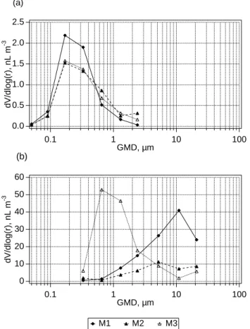
2.5 2.0 1.5 1.0 0.5 0.0 dV/dlog(r), nL m -3 0.1 1 10 100 GMD, µm 60 50 40 30 20 10 0 dV/dlog(r), nL m -3 0.1 1 10 100 GMD, µm (a) (b) M1 M2 M3
Fig. 1. Volume size distributions of sulphate (a) and sea-salt (b)
aerosols used in model simulations. Distributions for simulation M4 were identical to those for simulation M1.
size bin against dry deposition to the sea surface were based on Slinn and Slinn (1980). Emissions of sea-salt particles were equated to their dry-deposition fluxes thereby main-taining constant atmospheric concentrations. At each time step, fresh aerosol was added to, and an equivalent amount of reacted aerosol removed from, each sea-salt size bin in proportion to the corresponding atmospheric lifetime. This procedure sustained finite thermodynamic disequilibria for the internally mixed aerosols in each sea-salt size fraction; the magnitude of disequilibrium increased with particle size. During simulations, nss SO2−4 accumulated in both sea-salt and sulphate aerosols via dissolution and oxidation of SO2 and condensation of H2SO4.
Initial conditions for model runs are summarised in Ta-ble 1 and Fig. 1. Processes were simulated over a range of conditions to investigate multiphase variability in bromine species, differences in chlorine and bromine volatilisation as a function of particle size, and the sensitivity of O3to halo-gen chemistry.
3 Results and discussion
3.1 Meteorological condition summaries for intensive sam-pling periods
The meteorological data obtained on the tower and NO−3 and nss SO2−4 concentrations measured in cascade impactor sam-ples collected during each intensive are summarised in Ta-ble 2. The back-trajectories indicated that large-scale anticy-clonic flow of variable strength delivered air to the vicinity of the Hawaiian Islands throughout the experiment. No re-cent (i.e. within the five days represented by the trajectories) continental influence was suggested by any of the trajectories calculated for the first five intensive periods. During Inten-sive #6, however, the trajectories at all except the 9 km end-point level indicated relatively vigorous anticyclonic flow. A distinctive feature in this trajectory set was the 5 km end-point trajectories from the beginning of the period through 27 September, 00:00 UT, which suggested that air at this end-point altitude had passed close to and perhaps over the northwest U.S. – southwest Canadian shoreline at high alti-tude three to four days before arriving at the site. These 5 km endpoint trajectories suggested further that prior to about 4 days back, the air at this endpoint level may have been trans-ported rapidly across the mid-latitude North Pacific from Asia. The 27 September, 06:00 UT 5 km endpoint trajec-tories and subsequent ones indicated much less rapid, more localised flow. Nitrate and nss SO2−4 concentrations peaked later in the period (sample collected 27 September, 16:31 UT to 28 September, 04:10 UT). The back trajectories in combi-nation with the relatively high NO−3 and nss SO2−4 concentra-tions observed during this period strongly suggest that conti-nental pollutants were transported into the vicinity of Hawaii early during (and perhaps prior to) the period and then af-fected the air sampled near-surface after roughly a one-day delay.
3.2 Aerosol acidity
We inferred aerosol pH by evaluating the thermodynamic equilibrium between gas-phase HCl and aqueous Cl−. Re-sults are summarised in Table 3. Several potential sources of error are associated with this method. These include uncer-tainties in field measurements (HCl, particulate Cl−, RH and temperature), reliability of the hygroscopic growth models and associated assumptions involved in estimating aerosol LWCs, accuracy of Henry’s Law and acid dissociation con-stants for HCl, and the assumption that the multiphase sys-tem is at thermodynamic equilibrium with respect to HCl. Measurement uncertainties are described above and, in most cases, correspond to relatively minor sources of error in in-ferred acidity (<±0.1 pH unit). LWCs estimated using dif-ferent models (e.g. Gerber, 1985; Tang, 1997 for sea-salt) generally agree within about ±25% and, consequently, also
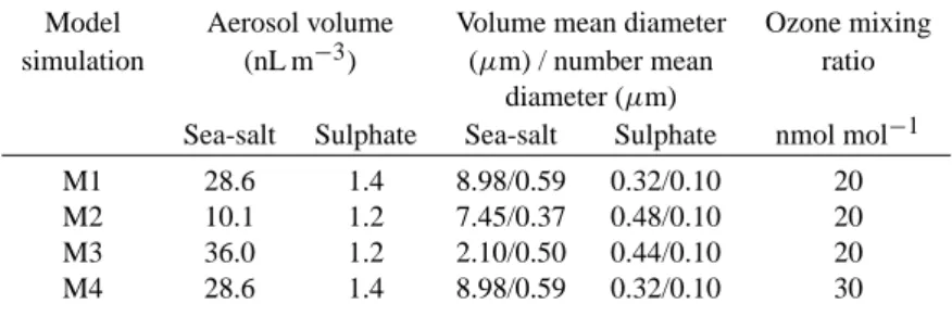
Table 1. (a) Description of aerosol and ozone mixing ratio in MOCCA model simulations.
Model Aerosol volume Volume mean diameter Ozone mixing
simulation (nL m−3) (µm) / number mean ratio
diameter (µm)
Sea-salt Sulphate Sea-salt Sulphate nmol mol−1
M1 28.6 1.4 8.98/0.59 0.32/0.10 20
M2 10.1 1.2 7.45/0.37 0.48/0.10 20
M3 36.0 1.2 2.10/0.50 0.44/0.10 20
M4 28.6 1.4 8.98/0.59 0.32/0.10 30
Table 1. (b) Initial conditions common to all MOCCA simulations.
General conditions temperature 297.65 K pressure 1013.25 hPa relative humidity 71.8 % latitude 21.35 degrees height of MBL 1000 m
Initial mixing ratios in gas phase
H2O2 600 pmol mol−1
NH3 100 pmol mol−1
NO2 20 pmol mol−1
HNO3 5 pmol mol−1
CH4 1.8 µmol mol−1
HCHO 300 pmol mol−1
CO 70 nmol mol−1
CO2 350 µmol mol−1
HCl 40 pmol mol−1
DMS 60 pmol mol−1
SO2 90 pmol mol−1
Alkenes 100 pmol mol−1
Alkanes 500 pmol mol−1
Concentrations in RH-equilibrated sea-salt particles∗
[Cl−] 5.75 M
[Br−] 0.0089 M
[HCO−3] 0.022 M
[SO=4] 0.30 M
Concentrations in RH-equilibrated sulphate particles∗
[HSO−4] + [SO=4] 3.61 M [NH+4] 1.81 M Emissions rates e eNO 0.024 g m−2year−1 eNH3 0.009 g m−2year−1 eDMS 0.082 g m−2year−1 ∗
Without Kelvin effect
correspond to relatively minor uncertainties in calculated aerosol acidity (<±0.1 pH unit, Keene and Savoie, 1998).
Uncertainty in the Henry’s Law constant for HCl corre-sponds to a potentially large source of error for this approach (Keene and Savoie, 1999). Published constants for HCl vary over three orders of magnitude (see Sander, 1999). The value used for the calculations reported herein (1.1 M atm−1, Marsh and McElroy, 1985) is similar to that reported by Brimblecombe and Clegg (1989) but is at the lower limit of published values. If the actual Henry’s Law constant for HCl is greater, aerosol acidities must be proportionately greater to sustain the measured phase partitioning. In this regard, we note that the average acidities of the super-µm sea-salt size fractions inferred from measured HCl phase partitioning under moderately polluted conditions at Bermuda (pH 3.5 to 4.5, Keene and Savoie, 1999) were within the range of indi-vidual detectable values estimated from direct acidity mea-surements under comparable conditions at the same location the following year (pH 3.3 to 5.5 with only two greater than 5.0, Keene et al., 2002). The consistency of these results sug-gests that the Henry’s Law constant adopted herein (and by Keene and Savoie, 1999) is probably close to the true value.
Finally, this approach is based on the evaluation of ther-modynamic equilibrium. Although sub-µm aerosols equi-librate rapidly with the gas phase, non-equilibrium condi-tions for the larger aerosol size fraccondi-tions (e.g. Meng and Seinfeld, 1996) could introduce bias in calculated acidities. However, kinetic models suggest that most sea-salt alkalinity in most remote marine regions is rapidly titrated and near-equilibrium pH is established within seconds to tens of min-utes after aerosol formation (Chameides and Stelson, 1992; Erickson et al., 1999). Corresponding lifetimes for most sea-salt aerosols against dry deposition are many hours to a few days. Although the chemical composition of recently acid-ified sea-salt continues to evolve toward equilibrium with the gas phase via incorporation of acids and volatilisation of HCl, model calculations indicate that aerosol pH is reg-ulated by HCl phase partitioning and, thus, under a given set of conditions, remains relatively constant after the initial alkalinity has been titrated (Keene and Savoie, 1998, 1999; Erickson et al., 1999). In addition, the super-µm aerosol
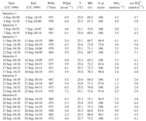
Table 2. Summary of meteorological and other ancillary data for each aerosol sample interval. Median values are given for meteorological
data obtained on the tower. NO−3 and nss SO2−4 values given are the sums over all stages of the cascade impactor sample collected during each intensive.
Start End WDir WSpd T RH % in NO3 nss SO2−4
(UT, 1999) (UT, 1999) (◦True) (m sec−1) (◦C) (%) sector (nmol m−3) (nmol m−3) Intensive 1 4 Sep, 04:50 4 Sep, 16:18 071 6.9 25.0 69.5 100. 4.3 4.7 4 Sep, 16:30 5 Sep, 05:00 070 6.6 25.3 67.2 100. 4.9 5.0 Intensive 2 7 Sep, 04:55 7 Sep, 16:07 063 4.8 25.1 74.9 100. 2.0 2.3 7 Sep, 16:19 8 Sep, 04:16 051 6.1 25.6 68.6 100. 3.5 4.5 Intensive 3 11 Sep, 04:30 11 Sep, 16:10 089 5.4 25.1 69.7 99.9 4.1 4.1 11 Sep, 16:30 12 Sep, 04:10 079 4.3 25.6 72.0 75.6 3.6 3.6 12 Sep, 04:30 12 Sep, 16:06 070 5.5 25.1 71.1 100. 3.3 3.9 12 Sep, 16:30 13 Sep, 04:00 064 5.9 25.6 68.7 100. 2.5 3.1 Intensive 4 16 Sep, 04:30 16 Sep, 16:09 077 6.8 25.2 69.3 100. 3.2 4.1 16 Sep, 16:36 17 Sep, 04:15 077 5.9 25.6 72.2 83.6 2.6 4.2 17 Sep, 04:25 17 Sep, 16:15 071 6.1 25.2 72.3 100. 3.0 4.5 17 Sep, 16:33 18 Sep, 04:10 073 5.9 25.8 70.3 98.6 3.4 4.8 Intensive 5 20 Sep, 16:30 21 Sep, 04:10 067 5.5 25.6 68.4 100. 1.5 2.6 21 Sep, 04:33 21 Sep, 16:10 067 5.4 24.8 71.3 97.0 1.2 2.0 21 Sep, 16:32 22 Sep, 04:15 073 6.5 25.5 70.0 100. 2.6 2.4 22 Sep, 04:39 22 Sep, 16:15 075 7.2 25.1 72.8 97.8 2.5 2.9 Intensive 6 26 Sep, 04:30 26 Sep, 16:10 085 6.3 25.3 75.1 96.9 3.2 3.8 26 Sep, 16:30 27 Sep, 04:10 073 5.3 25.8 74.9 100. 5.4 4.4 27 Sep, 04:36 27 Sep, 16:10 073 5.0 25.1 75.3 100. 4.7 5.0 27 Sep, 16:31 28 Sep, 04:10 058 4.0 25.5 66.0 93.9. 9.0 6.5 28 Sep, 05:28 28 Sep, 16:10 082 2.2 24.3 80.8 48.1 4.1 5.5 28 Sep, 16:30 29 Sep, 04:10 072 4.6 25.7 73.2 100. 3.3 4.1
size fractions at Hawaii exhibited small Cl−deficits relative to sea-salt (Table 3) and, consequently, the small (<20%) changes in aqueous Cl− concentrations between fresh and fully equilibrated sea-salt would have only minor influences on calculated acidities (<0.1 pH unit). Based on the above, the pHs of acidified aerosols estimated using this approach are probably reliable to about ±0.2 to ±0.3 pH unit.
The inferred equilibrium pHs for all aerosol size fractions analysed during the experiment were acidic (Table 3). Calcu-lated pHs for super-µm fractions ranged from 4.5 to 5.4 with a median value of 5.1. Acidities of 0.65-µm size fractions were relatively greater (median pH of 4.6) and more variable (Table 3). Most Cl− concentrations in the <0.65 µm size
fraction were less than the detection limit thereby precluding the application of this approach to estimate corresponding acidities. The greatest aerosol acidities during the experi-ment were associated with the apparent pollution transport episode on 28 September 1999. Aerosol pHs during that pe-riod fell within the upper range of reported values for mod-erately polluted conditions over the western North Atlantic Ocean (Keene and Savoie, 1999; Keene et al., 2002).
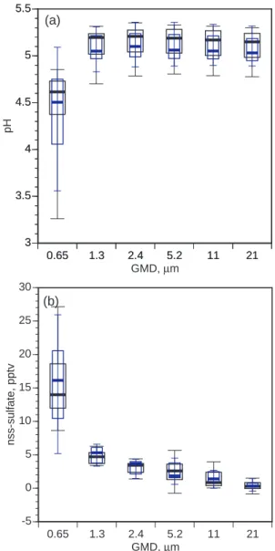
Laskin et al. (2003) recently hypothesized based on labo-ratory experiments that the reaction OH+Cl−→OH−+Cl at the surfaces of deliquesced sea-salt aerosols slows aerosol acidification and, thus, speeds S(IV) oxidation by O3 dur-ing daytime in clean marine air. Data generated durdur-ing this experiment were examined for evidence in support of this hy-pothesis. Median pH values inferred from HCl phase parti-tioning for each of the six largest size fractions did not differ statistically day vs. night (Mann-Whitney U tests, α=0.05), although the median in each fraction was 0.1 to 0.2 pH unit lower during the day than at night (Fig. 2a). Nss-SO2−4 dis-tributions also differed insignificantly day vs. night (Fig. 2b). Both of these observations are in agreement with MOCCA simulation results (Fig. 3b). HCl∗mixing ratios, with 2-hour time resolution, provide a diagnostic of aerosol acidity dur-ing midday. HCl is infinitely soluble in alkaline solution and its uptake is diffusion limited. Significant production of alkalinity during midday would favor HCl partitioning into the aerosol and, thus, smaller HCl mixing ratios in the gas phase. Systematic midday decreases in HCl∗ were not ev-ident (Fig. 4). Indeed, during the two cleanest sampling
0.65 1.3 2.4 5.2 11 21 3 3.5 4 4.5 5 5.5 pH GMD, µm 0.65 1.3 2.4 5.2 11 21 3 3.5 4 4.5 5 5.5 (a) 0.65 1.3 2.4 5.2 11 21 -5 0 5 10 15 20 25 30 nss-sulfate, pptv GMD, µm (b)
Fig. 2. Box-whisker plots of (a) aerosol pH during daytime (narrow
blue boxes) and nighttime (wide black boxes) inferred from HCl phase partitioning, and (b) measured nss-SO2−4 as a function of par-ticle size. Box tops and bottoms indicate quartile values, whiskers indicate decile values, and thick horizontal bars indicate median val-ues. Eleven daytime and eleven nighttime values were available for constructing each box.
periods (intensives 2 and 5, Table 2), HCl∗ mixing ratios peaked during midday (Fig. 4). These results suggest that the Laskin et al. (2003) mechanism of alkalinity production via surface reaction of OH with Cl−in sea-salt aerosols did not affect S cycling appreciably under these clean marine condi-tions.
The H++SO2−4 HSO−4 equilibrium resulted in most to-tal acidity existing as HSO−4 in all aerosol size fractions (Ta-ble 3, Saxena et al., 1993; Keene et al., 2002). Based on median values, total acidities were typically about 1.5 orders of magnitude greater than corresponding H+concentrations. In addition, all total acidities (expressed as − log10[H+tot]or
pHt) for the four largest size fractions fell within a narrow range of 2.9 to 3.6 over the variable conditions observed dur-ing this experiment (Table 3). It is evident from Eq. (2) that at the high concentrations of SO2−4 and low concentrations of H+that are typical of sea-salt aerosols (e.g. Table 3, Keene et al., 2002), the ratio [HSO−4]/[H+]is large and varies almost linearly with total [SO2−4 ]. Thus, the total acidity in sea-salt size fractions is determined in part by the total amount of SO2−4 present. Based on median values for the four largest size fractions, sea-salt accounted for 94% of total SO2−4 and sea-salt concentrations exhibited relatively little variability over the course of the experiment (Table 3). In addition RH varied within a fairly narrow range (Table 2) and, thus, wa-ter contents per unit sea-salt were similar across the super-µm size fractions (e.g. Gerber, 1985). Consequently, total [SO2−4 ] and total acidity exhibited relatively little variability across the four largest size fractions during the course of the experiment. Although HSO−4 represents a large fraction of total acidity in sea-salt aerosol solutions at Hawaii, absolute concentrations are low relative to the total amount of acid-ity in the entire multiphase system; gaseous acids (e.g. HCl) and sub-µm aerosol size fractions (Table 3) are the dominant reservoirs.
Equations (1) and (2) show that HCl mixing ratios and the sulphate equilibrium are directly coupled through H+.
For instance, combining and reorganising these expressions yields HClg {HSO−4} = {Cl −} {SO2−4 } × KaHSO− 4 KaHCl×KH . (3)
In all but the most polluted marine regions, Cl−and SO2−4 in sea-salt size fractions are present at concentrations close to sea-salt ratios and, consequently, the right side of the equa-tion exhibits relatively little variability over the global MBL. Thus, the left side of the equation must also be relatively constant. This relationship provides useful context for com-paring aerosol acidities across variable chemical regimes.
Median total acidities (expressed as pHt) for the four largest size fractions at Hawaii (3.3 to 3.4, Table 3) were within the range of those observed in association with higher levels of pollutants at Bermuda (2.7 to 3.5, Keene et al., 2002). In contrast, the corresponding median H+ activities
(expressed as pH) at Hawaii (5.1 for all size fractions, Ta-ble 3) were less than those at Bermuda (4.1 to 4.6, Keene et al., 2002). As was the case at Hawaii, sea-salt accounted for most (93%) of total SO2−4 in the four largest size frac-tions at Bermuda and corresponding median concentrafrac-tions of total SO2−4 (6.9 nmol m−3, Keene et al., 2002) were sim-ilar to those at Hawaii (5.3 nmol m−3). However, RHs at Bermuda (median=91% for the subset of samples with de-tectable acidities, Keene et al., 2002) were greater than those at Hawaii (Table 2). Consequently, aqueous concentrations of [SO2−4 ], [HSO−4], and corresponding equilibrium ratios of [HSO−4]/[H+] for detectable acidities at Bermuda were also
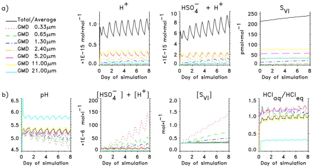
Fig. 3. Mixing ratios (a) and aqueous concentrations (b) in sea-salt aerosol simulated in M1. For HCl the ratio [HCl]aq/[HCl]eqis shown,
where the denominator is the equilibrium concentration with gas-phase HCl.
700 600 500 400 300 200 100 0 -100 pmol Cl mol -1 275 270 265 260 255 250 245
Julian Day, 1999 (UT)
Fig. 4. Measured mixing ratios of HCl∗(blue) and Cl∗(red) and corresponding Cl−deficits (black) summed over the impactor size fractions. All Cl∗ values were below a detection limit of about 20 pmol mol−1during the first two intensive sampling periods. The lower detection limit of approximately 6 pmol mol−1during the rest of the experiment is indicated by the thin black line drawn from JD 253 to JD 273. Error bars for HCl∗and Cl∗correspond to preci-sions stated in the text. For Cl−deficits the horizontal error bars correspond to the sampling intervals and the vertical error bars rep-resent the propagated precisions associated with the 14 individual measurements (7 Cl−and 7 Mg2+) underlying each sum. Shaded vertical bands indicate nighttime (sunset to sunrise) intervals during each intensive sampling period.
lower. The influences of higher solution [H+] and higher aerosol water content on [HSO−4] at Bermuda relative to Hawaii were of comparable magnitude but opposite direction resulting in similar median total acidities in the four largest size fractions at the two sites. Although not measured at Bermuda during Spring 1997, we would predict from Eq. (3) that the corresponding HClgmixing ratios during that period were within the same range as those at Hawaii (Table 3). HClg mixing ratios under conditions of lower RH (79% to 93%) at Bermuda during Spring 1996 ranged from 133 to 883 pmol mol−1 (Keene and Savoie, 1998), which overlap the range of values at Hawaii.
Sea-salt aerosol pHs simulated by MOCCA were gener-ally in agreement with those inferred from thermodynamic relationships with simulated values for most size fractions ranging between 4.9 and 5.5 (Fig. 3b). The corresponding range of pHs of super-µm size fractions inferred from ther-modynamic relationships was 4.5 to 5.4 (Table 3). However, pHs for the largest size fraction in model simulations oscil-lated around a somewhat higher value of 5.9 due primarily to the rapid turnover rates and relatively larger infusions of alkalinity associated with fresh sea-salt aerosols. The con-stant production of new aerosols by wave action and the constant removal of reacted aerosols via deposition sustains dynamic disequilibria in both the model and in the ambient MBL. Larger size fractions have short lifetimes against depo-sition (in the model, 43, 18 and 8 h, respectively for particles with diameters 5.2, 11 and 21 µm). The corresponding times required to titrate sea-salt alkalinity and to acidify particles of these sizes to near equilibrium pHs were approximately 0.5, 2 and 6 h, respectively. For the largest size fraction, the
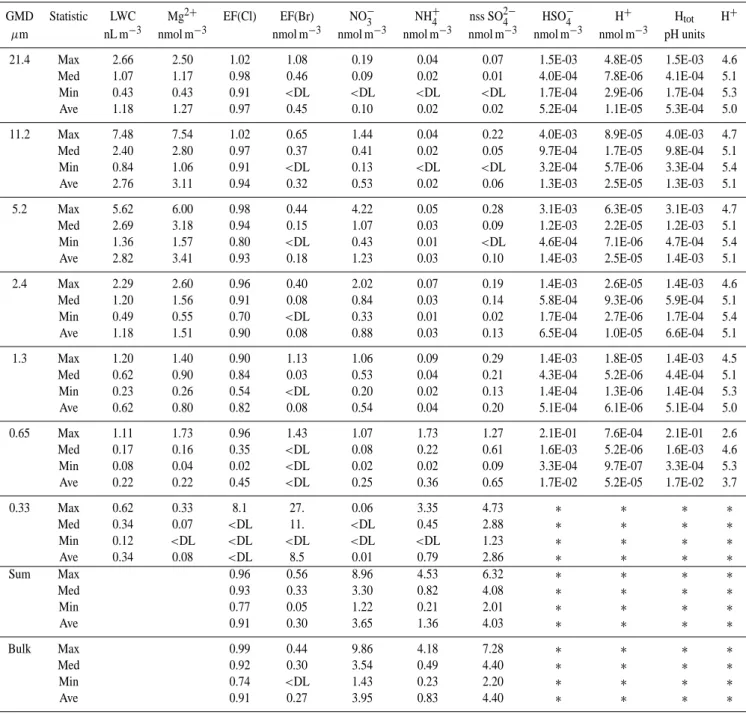
Table 3. Summary statistics for size-segregated aerosol composition at Hawaii during summer (N=22).
GMD Statistic LWC Mg2+ EF(Cl) EF(Br) NO−3 NH4+ nss SO2−4 HSO−4 H+ Htot H+
µm nL m−3 nmol m−3 nmol m−3 nmol m−3 nmol m−3 nmol m−3 nmol m−3 nmol m−3 pH units
21.4 Max 2.66 2.50 1.02 1.08 0.19 0.04 0.07 1.5E-03 4.8E-05 1.5E-03 4.6
Med 1.07 1.17 0.98 0.46 0.09 0.02 0.01 4.0E-04 7.8E-06 4.1E-04 5.1
Min 0.43 0.43 0.91 <DL <DL <DL <DL 1.7E-04 2.9E-06 1.7E-04 5.3
Ave 1.18 1.27 0.97 0.45 0.10 0.02 0.02 5.2E-04 1.1E-05 5.3E-04 5.0
11.2 Max 7.48 7.54 1.02 0.65 1.44 0.04 0.22 4.0E-03 8.9E-05 4.0E-03 4.7
Med 2.40 2.80 0.97 0.37 0.41 0.02 0.05 9.7E-04 1.7E-05 9.8E-04 5.1
Min 0.84 1.06 0.91 <DL 0.13 <DL <DL 3.2E-04 5.7E-06 3.3E-04 5.4
Ave 2.76 3.11 0.94 0.32 0.53 0.02 0.06 1.3E-03 2.5E-05 1.3E-03 5.1
5.2 Max 5.62 6.00 0.98 0.44 4.22 0.05 0.28 3.1E-03 6.3E-05 3.1E-03 4.7
Med 2.69 3.18 0.94 0.15 1.07 0.03 0.09 1.2E-03 2.2E-05 1.2E-03 5.1
Min 1.36 1.57 0.80 <DL 0.43 0.01 <DL 4.6E-04 7.1E-06 4.7E-04 5.4
Ave 2.82 3.41 0.93 0.18 1.23 0.03 0.10 1.4E-03 2.5E-05 1.4E-03 5.1
2.4 Max 2.29 2.60 0.96 0.40 2.02 0.07 0.19 1.4E-03 2.6E-05 1.4E-03 4.6
Med 1.20 1.56 0.91 0.08 0.84 0.03 0.14 5.8E-04 9.3E-06 5.9E-04 5.1
Min 0.49 0.55 0.70 <DL 0.33 0.01 0.02 1.7E-04 2.7E-06 1.7E-04 5.4
Ave 1.18 1.51 0.90 0.08 0.88 0.03 0.13 6.5E-04 1.0E-05 6.6E-04 5.1
1.3 Max 1.20 1.40 0.90 1.13 1.06 0.09 0.29 1.4E-03 1.8E-05 1.4E-03 4.5
Med 0.62 0.90 0.84 0.03 0.53 0.04 0.21 4.3E-04 5.2E-06 4.4E-04 5.1
Min 0.23 0.26 0.54 <DL 0.20 0.02 0.13 1.4E-04 1.3E-06 1.4E-04 5.3
Ave 0.62 0.80 0.82 0.08 0.54 0.04 0.20 5.1E-04 6.1E-06 5.1E-04 5.0
0.65 Max 1.11 1.73 0.96 1.43 1.07 1.73 1.27 2.1E-01 7.6E-04 2.1E-01 2.6
Med 0.17 0.16 0.35 <DL 0.08 0.22 0.61 1.6E-03 5.2E-06 1.6E-03 4.6
Min 0.08 0.04 0.02 <DL 0.02 0.02 0.09 3.3E-04 9.7E-07 3.3E-04 5.3
Ave 0.22 0.22 0.45 <DL 0.25 0.36 0.65 1.7E-02 5.2E-05 1.7E-02 3.7
0.33 Max 0.62 0.33 8.1 27. 0.06 3.35 4.73 ∗ ∗ ∗ ∗ Med 0.34 0.07 <DL 11. <DL 0.45 2.88 ∗ ∗ ∗ ∗ Min 0.12 <DL <DL <DL <DL <DL 1.23 ∗ ∗ ∗ ∗ Ave 0.34 0.08 <DL 8.5 0.01 0.79 2.86 ∗ ∗ ∗ ∗ Sum Max 0.96 0.56 8.96 4.53 6.32 ∗ ∗ ∗ ∗ Med 0.93 0.33 3.30 0.82 4.08 ∗ ∗ ∗ ∗ Min 0.77 0.05 1.22 0.21 2.01 ∗ ∗ ∗ ∗ Ave 0.91 0.30 3.65 1.36 4.03 ∗ ∗ ∗ ∗ Bulk Max 0.99 0.44 9.86 4.18 7.28 ∗ ∗ ∗ ∗ Med 0.92 0.30 3.54 0.49 4.40 ∗ ∗ ∗ ∗ Min 0.74 <DL 1.43 0.23 2.20 ∗ ∗ ∗ ∗ Ave 0.91 0.27 3.95 0.83 4.40 ∗ ∗ ∗ ∗
Average Cl−and Br−enrichment factors based on average Mg2+and average Cl−and Br−, respectively, for all samples.
∗Particulate Cl−concentrations below detection limit; acidities and HSO−4 cannot be inferred.
turnover rate and the rate of alkalinity titration are of similar magnitude and, consequently, the thermodynamic approach overestimates acidities of the largest particles.
The last panel in Fig. 3 depicts the equilibrium state of the modeled sea-salt particles with respect to HCl. From Eq. (1) the y-axis equals {H+}×{Cl−}/({H+}×{Cl−})eq. Be-cause {Cl−}is many orders of magnitude larger than {H+},
{Cl−}/{Cl−}eq ≈1 for the equilibrium in question and the ratio on the y-axis reflects variations in {H+}/{H+}eq. The panel shows that {H+} in the largest size fraction was 3– 5 times lower (0.5–0.7 pH unit) than the equilibrium value with respect to HCl. The size fractions with diameter 5.2 µm and smaller became slightly supersaturated and released HCl to the gas phase. Initially the supersaturation was larger
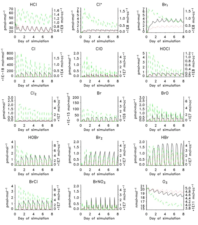
Fig. 5. Simulated mixing ratios of some halogen species and ozone in the gas phase in model runs M1 (black), M2 (red), and M3 (green).
for small particles because they absorb acids faster and be-cause the ocean-atmosphere exchange process that intro-duces fresh, undersaturated sea-salt particles is slower. Act-ing in opposition to the absorption of acids is the halogen ac-tivation mechanism described by (R1) and (R2), which con-sumes acidity. Since the halogen cycling is more intensive in small particles, their supersaturation successively decreases relative to the larger particles and they even become under-saturated.
3.3 Halogen cycling
Measured mixing ratios of HCl∗ (primarily HCl)
aver-aged 100 pmol mol−1and varied from below detection limit (30 pmol mol−1) to 250 pmol mol−1; those of Cl∗ (Cl radi-cals, Cl2, and HOCl) averaged 6 pmol mol−1and varied from below detection limit (about 3 pmol mol−1for most of the ex-periment) to 38 pmol mol−1(Fig. 4). The maximum average mixing ratios of HCl∗ and Cl∗ over 12-hour periods (day-and nighttime) were 199 (day-and 12 pmol mol−1, respectively, and occurred during daytime. Based on all measurements,
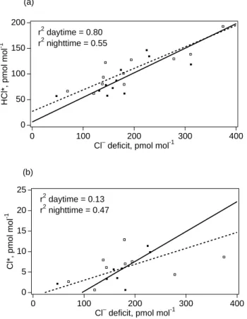
25 20 15 10 5 0 Cl*, pmol mol -1 400 300 200 100 0
Cl– deficit, pmol mol-1 r2 daytime = 0.13 r2 nighttime = 0.47 200 150 100 50 0 HCl*, pmol mol -1 400 300 200 100 0
Cl– deficit, pmol mol-1 r2 daytime = 0.80
r2 nighttime = 0.55 (a)
(b)
Fig. 6. Mixing ratios of HCl∗(a) and Cl∗ (b) averaged over
im-pactor sampling intervals plotted against corresponding measured particulate Cl−deficits summed over all impactor stages (daytime: open squares; nighttime:solid squares). Lines are regressions for daytime (dashed) and nighttime (solid), respectively, calculated by the reduced major axis method (Hirsch and Gilroy, 1984). Regres-sion coefficients: HCl∗vs. Cl−deficit daytime: slope=0.42, inter-cept=27; nighttime: slope=0.48, intercept=6.3; Cl∗vs. Cl−deficit daytime: slope=0.039, intercept=−0.9; nighttime: slope=0.073, intercept=−7.0.
mean mixing ratios of both HCl∗and Cl∗were slightly higher during daytime.
The simulated mixing ratios of HClg and Cl∗ varied be-tween 20 and 70 pmol mol−1, and 0.5 and 6 pmol mol−1, re-spectively (Fig. 5), which are near the lower ends of the ranges of the respective measured concentrations. The higher mixing ratios during the latter part of the experiment were as-sociated with the pollution episode and are not representative of the cleaner conditions considered in the simulations. The simulated HClgconcentrations increased during the daytime, peaked before dusk, and decreased overnight to minimum values at dawn. Afternoon maxima in measured HCl∗ con-centrations were observed on some days but a consistent diel pattern was not evident over the course of the experiment.
Simulated ClO, HOCl and Cl peaked during daytime while simulated Cl2peaked at night. The net effect is relatively little diel variability in simulated Cl∗ (Fig. 5). Absolute
concentrations of simulated Cl∗and associated diel patterns
also differed among the cases studied. Simulation M1 in-dicated lower nighttime concentrations and an early morning minimum whereas simulation M3 indicated a nighttime max-imum.
In the following discussion, particulate halogen “ex-cesses” and “deficits” refer to absolute departure from sea water composition (i.e. nmol or pmol m−3) while the terms “enrichment” and “depletion” refer to relative deviations. The measured particulate Cl−deficits summed over all im-pactor stages do not show any clear diel variability (Fig. 4). The temporal variability over the course of the campaign re-sembled that of HCl∗ with larger deficits measured towards the end in association with high levels of pollutants. HCl∗ mixing ratios were strongly positively correlated to partic-ulate Cl− deficits during daytime and less strongly
corre-lated at night, while correlations of Cl∗mixing ratios to Cl−
deficits were weak or insignificant (Fig. 6).
The simulated Cl− enrichments (EFCl=
(Cl−/Mg2+)sample/(Cl−/Mg2+)seawater) in sea-salt par-ticles were between 0.95 and 0.80, indicating Cl−depletions similar to observed values. The Cl−enrichment of sub-µm particles was between 0.75 and 0.25, indicating less Cl− depletion than was observed; median measured enrichments were 0.35 and essentially zero for the 0.65 and 0.33 µm fractions, respectively (Table 3). This difference can be ex-plained partly by the fact that the simulated sea-salt particles were externally mixed with sulphate particles at initialisation and did not physically mix during the model runs. They were therefore less acidic than actual sub-µm particles. The simulated diel pattern of the total (summed over all aerosol size fractions) Cl− deficit showed a maximum rate
of increase during afternoon and minimum at night (Fig. 7), which is consistent with diel variability indicated by the measurements (Fig. 4).
Mixing ratios of total gaseous inorganic Br (Brt) varied from below detection limits (1.5–2 pmol mol−1) to 9 pmol mol−1 (Fig. 8a) with average mixing ratio 3.7 pmol mol−1. The maximum values were measured dur-ing daytime and the mean for mixdur-ing ratios durdur-ing day-time was greater than that for nightday-time. Mixing ratios also varied temporally over the course of the experiment in a similar way as Cl∗ (compare Fig. 4). The particulate Br− deficit in bulk samples, expressed as mixing ratios, varied from 1 to 6 pmol mol−1with average value 3.2 pmol mol−1. Like Brt, highest individual Br−deficits and a higher mean deficit were measured during the daytime. The nighttime Br− deficit data were positively correlated to Br
t while the daytime data were not (Fig. 9).
Maximum simulated mixing ratios of Brt varied between 1.5 and 7.0 pmol mol−1(Fig. 5), which are within the range of measured concentrations (Fig. 8). The higher values were associated with the higher concentrations of sea-salt particles in simulation M3. Maximum simulated mixing ratios of in-dividual Br species (HBr, HOBr, BrO, BrCl, and Br2were
Fig. 7. Simulated concentrations of Cl−and Br−enrichment factors in sea-salt aerosols for model runs M1 (a) and M3 (b).
each in the range of a few (1.5 to 3.0) pmol mol−1; HBr, HOBr and BrO peaked during daytime and BrCl and Br2 peaked at night. In all cases, Brt mixing ratios were high-est in the early morning and lowhigh-est at dusk. In simulations M1 and M2 the Brtmixing ratio increased slowly overnight whereas, in simulation M3, the Brt mixing ratio increased quickly after dusk. These differences account for higher av-erage daytime mixing ratios of Brt in simulations M1 and M2 compared to higher average nighttime mixing ratios in simulation M3. The diurnal variabilities of Brt in the model are thus quite in agreement with measurements, with higher daytime Brtmixing ratio on average but with some occasions when daytime mixing ratios were lower than those during the following night. Von Glasow et al. (2003) investigated the diurnal variability of Brt with the 1-dimensional model MISTRA and found that presence of clouds influenced diur-nal variability of Brt. In simulations with clouds, Br2 and BrCl, which would otherwise accumulate in the gas phase, dissolved into the cloud droplets causing nighttime minima in mixing ratios of these two compounds.
Diurnal variability in Br−and EFBr also differed between
simulations M1 and M2 relative to M3. Under the conditions of less intensive halogen cycling, the bromine volatilisation took place only during daytime when there were significant concentrations of HOBr driving the Br activation reaction R1. In simulation M2 no volatilisation took place at night and the EFBr increased due to the continuous air-sea exchange in the model replacing the bromine-depleted sea-salt particles
with fresh ones. In simulations M1 and M3 with more inten-sive halogen cycling, larger gas phase mixing ratios of BrCl and Cl2developed after dusk and bromine volatilisation oc-curred as BrCl and Cl2 dissolved into the sea-salt aerosol, volatilising Br2. In M3 with slower air-sea exchange this nighttime volatilisation led to the lower nighttime mixing ra-tios of Br− (and decreased EFBr) compared to daytime. In M1 with faster air-sea exchange the nighttime volatilisation was smaller than the relative increase of Br−due to air-sea
exchange, and the diurnal pattern was similar to that of sim-ulation M2. Differences between diurnal variabilities in M1 and M3 can be seen in Fig. 7. The model results can be com-pared to the measured Br− deficits (Fig. 8b) with slightly larger deficits during daytime than at night on average. Von Glasow and Crutzen (2003) recently compared diurnal cy-cles of Br−in 1-D MISTRA model simulations with inten-sive and less inteninten-sive bromine volatilisation. They obtained opposite diurnal cycles in agreement with our simulations, however with much larger amplitude in a low Br− volatili-sation case. Rancher and Kritz (1980) reported diurnal vari-abilities of Brt and Br−over the equatorial Atlantic Ocean with consistently higher Brtand lower Br−during daytime.
Measured mixing ratios of BrO were less than detection limits of ≈2 pmol mol−1 throughout the experiment, which is consistent with model predictions (Fig. 5). To examine if a diel cycle in BrO can be discerned, data for changes in BrO mixing ratios over 3-hour periods, which generally have smaller uncertainties as noted above, were plotted over
(a) (b) 20 15 10 5 0 -5 -10 Br
– deficit, pmol mol
-1 275 270 265 260 255 250 245 Julian Day 12 10 8 6 4 2 0 Br t , pmol mol -1 275 270 265 260 255 250 245 Julian Day, UT
Fig. 8. Measured mixing ratios of (a) Brt and (b) corresponding
Br− deficits in bulk aerosol during daytime (red) and nighttime (black); detection limits for Brtare indicated with horizontal dashed
lines in panel a. The widths of the red and black dash symbols cor-respond to the sampling intervals. Vertical error bars corcor-respond to precisions stated in the text.
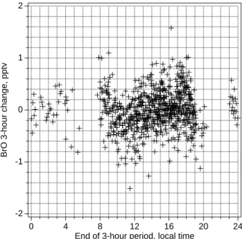
local time of the day (end of the 3-hour period) (Fig. 10). All data were lower than their respective detection limits, which reached as little as 0.5 pmol mol−1 when visibility was excellent. Only data with detection limits lower than 2 pmol mol−1 were considered. The data scattered around zero, however, changes in BrO mixing ratio during the 3-hour period ending at 11:00 local time were mostly negative, aver-aging −0.3 pmol mol−1, which would be consistent with de-creasing BrO mixing ratios during morning as simulated by MOCCA (Fig. 5). Evaluated BrO mixing ratios lower than the detection limit have to be taken with great care, as they may result from systematic features in the DOAS spectra, caused by diurnal changes of the lamp emission structures or by changes in trace gases absorbing in the wavelength re-gion covered by the spectrum. Nonetheless, plots of changes of other trace gas concentrations as measured by DOAS do not show any noticeable diurnal variations, indicating that the uncertainty of the evaluation is mostly caused by random noise in the spectra.
12 10 8 6 4 2 0 -2 Br t , pmol mol -1 20 15 10 5 0 -5 -10
Br– deficit, pmol mol-1 r2 daytime = 0.016
r2 nighttime = 0.74
Fig. 9. Measured mixing ratios of Brt versus corresponding Br−
deficits in bulk aerosol during the daytime (red) and nighttime (black). Error bars correspond to precisions stated in the text. Slanted lines are regressions for daytime (red dashed) and nighttime (black solid), respectively, calculated by the reduced major axis method (Hirsch and Gilroy, 1984). Regression parameters are as follows: Brtvs. Br−deficit daytime: slope=1.84, intercept=−1.40;
Brtvs. Br−deficit nighttime: slope=1.12, intercept=−0.86.
-2 -1 0 1 2
BrO 3-hour change, pptv
24 20 16 12 8 4 0
End of 3-hour period, local time
Fig. 10. Changes in BrO mixing ratios over a nominal 3-hour period
plotted versus local time of end of the 3-hour period. Actual time differences between the two spectra used varied between 2.5 and 3.5 hours. All values were lower than their respective detection limits.
The measured Br− concentrations and enrichments
rela-tive to sea salt indicate that most of the super-µm size frac-tions were depleted in Br−(Table 3, Fig. 11). Bromide de-pletion increased with decreasing diameter from an average EF of about 0.5 for the >21 µm size fraction to 0.09 for the 2.4 µm size fraction. The 2.4 µm and 1.3 µm size fractions of most samples were almost completely depleted in Br−. The smallest size fractions were typically enriched in Br− relative to sea-salt (EFBr>1 for most of the samples).
(a) (b) 0.6 0.4 0.2 0.0 Br – , pmol mol -1 3 4 5 6 7 1 2 3 4 5 6 7 10 2 GMD, µm -1.0 -0.5 0.0 0.5 1.0 EF Br for GMD > 0.33 µm 3 4 5 6 7 1 2 3 4 5 6 7 10 2 GMD, µm 25 20 15 10 5 0 -5 EF Br for GMD = 0.33 µm
Fig. 11. Average particulate Br−enrichment factors (a) and mixing ratios (b) as a function of size based on measured concentrations during daytime (red) and nighttime (black). Error bars are ±1 stan-dard deviation of the eleven values from which the averages were calculated for each point plotted. Daytime values are slightly offset horizontally to reduce overlap. Note the different scale for EFBr for the 0.33 µm size fraction in panel a.
The measured and simulated Br−enrichments were com-parable for most size fractions. Simulated enrichments inte-grated over all size fractions were between 0.6 and 0.9 and decreased from ≈0.95 in the largest particles to ≈0.05 in the 2.4 µm size bin (Figs. 7 and 11). However, the measured excess of Br−in smallest size fraction (GMD 0.33 µm, Ta-ble 3) was not reproduced by the model. The simulated sub-µm sea-salt particles lost their bromine almost entirely. Ex-ternally mixed sulphate particles accumulated some bromine but this gain was at most 20 times less than the corresponding loss from similarly sized sea-salt particles.
Most of the measured particle mass in the sub-µm size fraction is contributed by SO2−4 , NH+4 and associated H2O (e.g. Table 2). These fine particles are also enriched in potas-sium and sometimes calcium relative to sea-salt, presum-ably due to terrestrial or combustion sources of K and Ca. Most sub-µm aerosols (or their surface layers) in the Hawai-ian MBL are presumably hydrated and acidic so any asso-ciated Br− should recycle, which makes it difficult to ex-plain the enrichment by inorganic Br of non-marine origin. One possibility is that the Br−is associated with chemically distinct particles, e.g. particles originating from combustion of leaded fuel in East-Asian vehicle fleets or particles
origi-nating from biomass burning. The highest Br−enrichments
were observed in association with the presence of significant pollutants, which trajectories suggest may have been trans-ported from Asia. Alternatively, MOCCA may be missing some important process that leads to accumulation of
sub-µm Br−. See Sander et al. (2003) for further discussion of
inorganic bromine chemistry in the MBL.
3.4 Interactions among halogens, ozone and nitrogen com-pounds
Sensitivity of the model to O3 mixing ratio was explored. When the initial mixing ratio of O3was increased from 20 (simulation M1) to 30 nmol mol−1(simulation M4), mixing ratios of reactive halogen species in the gas phase also in-creased (Fig. 12). Bromide depletions of sea-salt particles increased by up to 8%. Observed O3variations between 15 and 35 nmol mol−1 during the campaign may thus explain some of the variability in the measured halogen species. Gas-phase inorganic halogens reduce O3concentrations, making the sea-salt aerosol a catalytic reactor for O3 destruction. This effect can be seen by comparing O3in simulations M2 and M3 (see Fig. 5). The O3mixing ratio at the end of sim-ulation M3 with high sea-salt is 16 nmol mol−1while in M2, with the lowest sea-salt mixing ratio, the O3mixing ratio is 19 nmol mol−1. The ≈25% increase in sea-salt mixing ratio corresponds to a 16% O3decrease.
The role of the sea-salt particles in O3chemistry is rather complex. Ozone is destroyed catalytically by Br via reac-tions (R3) to (R5) and to some extent by the analogous Cl re-actions. Reactions (R4) and (R5) convert HO2to OH, which also leads to O3destruction via the HOxcycle:
OH+O3→HO2+O2 (R6)
HO2+O3→OH+2O2 (R7)
These O3losses are partly offset by formation through reac-tions with NO
XO+NO→X+NO2 (X=OH, Br, Cl) (R8)
followed by NO2photolysis
NO2+hν→NO+O. (R9)
Ozone losses by various pathways were calculated in sim-ulations M1 and M3 to quantify the effect of halogens on MBL O3concentration. In Fig. 13, the diel variation of O3 loss due to (R3) plus its Cl analog is compared to losses due to O3photolysis and the HOxand NOxcycles. The contri-bution from (R8) was not subtracted from that of (R3) and was plotted separately because this reaction simultaneously contributes to O3 formation in the NOx cycle. Photolysis is the most important O3sink with a magnitude of approx-imately 1500 pmol O3mol−1day−1. In MOCCA this sink is approximately compensated by the stratospheric contribu-tion. Figure 13 shows that the halogens deplete O3 in the
Fig. 12. Simulated mixing ratios of some halogen species and ozone in the gas phase in model runs M1 (black) and M4 (red, dotted).
MBL to an extent similar to that of the HOxcycle (200 to 700 pmol mol−1day−1). Increasing sea-salt aerosol concen-tration (and particle surface area) from that in simulation M1 to that in M3, increases O3depletion by approximately a fac-tor of two. Dry deposition of O3 to the sea surface was of similar magnitude to that of the HOx-cycle sink in both sim-ulations. At the same time, photochemical O3formation de-creased by a factor of 2 from 1540 to 790 pmol mol−1day−1 at the beginning of simulation M3. This decrease was caused by more intensive removal of NOxfrom the gas phase, which
was mainly caused by heterogeneous reaction of BrNO3with sea-salt particles. It is the coupling between NOxand halo-gen cycles that makes the sea-salt – O3interaction complex. Halogen nitrates are formed through
XO+NO2→XNO3(X=Br, Cl). (R10)
In the model these nitrates react with liquid aerosols (Sander et al., 1999):
XNO3+H2O(l)→HOX+HNO3 (R11)
Fig. 13. Diel cycles of different ozone sinks from simulations M1 (a) and M3 (b). Negative values imply net ozone production.
Nitric acid can be reduced to NO2in the gas phase by pho-tolysis and by reaction with OH. In the aqueous phase, NO−3 can be photolysed to NO2and OH.
The budgets of different NOx sinks are compared in Fig. 14. The gas-phase sinks were mainly reaction of NO2 with OH (55 to 60%) and reaction of DMS with NO3. Gas-phase reduction of HNO3 to NO2 was unimportant in both model simulations (0.2 pmol mol−1day−1 in
maxi-Fig. 14. Diel cycles of different sinks of NOxfrom simulations M1 (a) and M3 (b). Negative values are sources from NO−3 photolytic reduction in sea-salt particles.
mum). The heterogeneous sink of NO2(R10) was followed by (R11) or (R12) with BrNO3responsible for 80 to 95% of the integrated 24-hour loss of NOxthrough (R10) to (R12). On sea-salt particles the most important heterogeneous reac-tion of BrNO3was reaction with Cl− while on the sulphate particles it was hydration. In sea-salt particles a few pmol mol−1 day−1 of NO−3 were reduced back to NO2 through photolysis. This reaction was negligible in sulphate particles.