HAL Id: hal-00877479
https://hal.archives-ouvertes.fr/hal-00877479
Submitted on 28 Oct 2013
HAL is a multi-disciplinary open access archive for the deposit and dissemination of sci-entific research documents, whether they are pub-lished or not. The documents may come from teaching and research institutions in France or abroad, or from public or private research centers.
L’archive ouverte pluridisciplinaire HAL, est destinée au dépôt et à la diffusion de documents scientifiques de niveau recherche, publiés ou non, émanant des établissements d’enseignement et de recherche français ou étrangers, des laboratoires publics ou privés.
one-dimensional cases?
Éric Lantz, François Vernotte
To cite this version:
Éric Lantz, François Vernotte. Can we define a best estimator in simple one-dimensional cases?. IEEE Signal Processing Magazine, Institute of Electrical and Electronics Engineers, 2013, 30, pp.151 - 156. �10.1109/MSP.2013.2276532�. �hal-00877479�
in simple 1-D cases ?
´
Eric Lantz and Franc¸ois Vernotte
I. SCOPE
What is the best estimator for assessing a parameter of a probability distribution from a small number of measurements? Is the same answer valid for a location parameter like the mean as for a scale parameter like the variance? It is sometimes argued that it is better to use a biased estimator with low dispersion than an unbiased estimator with a higher dispersion. In which cases is this assertion correct ? In order to answer these questions, we will compare on a simple example the determination of a location parameter and a scale parameter with three “optimal” estimators: the minimum-variance unbiased estimator, the minimum square error estimator and the a posteriori mean.
II. RELEVANCE
Nowadays, it seems that processing a huge amount of data is a very common task. However, in some cases it is of great importance of being able to assess the statistical parameters of a process from a very small number of measurements. This can occur for instance in the analysis of the very long term behavior of time series (e.g. amplitude estimation of very low frequencies, time keeping, etc.). This paper focuses on the choice of the best estimator to be used over, say, less than 10 measurements.
III. PREREQUISITES
The reader is expected to have a basic understanding of data statistical processing, such as the one developed in [1].
E. Lantz is with Department of Optics, Femto-ST, University of Franche-Comt´e/CNRS, UFR Sciences - Route de Gray, 25030 Besanc¸on Cedex - France (Email: [email protected]).
F. Vernotte is with UTINAM, Observatory THETA of Franche-Comt´e, University of Franche-Comt´e/CNRS, 41 bis avenue de l’observatoire - B.P. 1615, 25010 Besanc¸on Cedex - France.
IV. PROBLEM STATEMENT
A. Two examples of measurement
We consider in this note the simplest archetypal measurement situation: an unknown quantity µ is measured N times, giving N measurements forming a set {di, i = 1 . . . N }, noted {di} in the following. Each measurement may be written as
di = αµ + ni (1)
where
• αµ is the deterministic part: α is a known constant1, |α| ≤ 1, and µ a parameter we want
to estimate;
• ni is the random part which is supposed to be a zero-mean additive white Gaussian noise, of unknown variance σ2, independent from one measurement to another.
In the following, we discuss successively the estimation of the two unknown parameters ap-pearing in this measurement process. The generic name of the unknown parameter will be θ, corresponding respectively to:
• (Example 1) θ = µ. In this first example, θ can be either positive or negative and is called
a location parameter, since the probability density of the data di can be expressed as a function of the difference of location |di− αθ|.
• (Example 2) θ = σ2. This variance is positive and is called a scale parameter since it
determines the precision scale relevant for the measurement of the location parameter of the measurement process.
Before going further to the definition of estimators, let us recall the heuristic concepts of location parameter versus scale parameter and model world versus measurement world.
B. Location parameter and scale parameter
Let us consider a random variable d which depends on a parameter θ. Let us denote pθ(d) its probability density function (PDF).
1For rendering this example relevant, we ought to keep in mind that α can be frequency dependent. For instance, α may be
a transfer function H(f ) of a measurement apparatus for a given frequency f , if θ is the Fourier transform for this frequency of a time varying signal.
1) Location parameter: A location parameter is a parameter whose variation induces a shift of the PDF of a random variable which depends of it. It is an additive parameter.
Let us denote p0(d) the PDF obtained for θ = 0:
pθ(d) = p0(d − θ). (2)
The mean and the median of a normal distribution are location parameters.
2) Scale parameter: A scale parameter is a positive parameter which controls the flattening or the narrowness of a PDF, for example the variance of a normal distribution. It is a multiplicative parameter. Let us denote p1(d) the PDF of the estimator of this parameter, obtained for θ = 1. We have : pθ(d) = 1 θp1 µ d θ ¶ . (3)
p1(d) is for example a χ2 distribution ifd is the estimator of the variance of a normal distribution.
C. Model world and measurement world
Two problems are generally addressed: the direct problem, which aims to forecast the measure-ment data knowing the parameter and the inverse problem, which aims to estimate the parameter knowing the measurement data. In the same vein, Tarantola distinguishes the model space, i.e. the space in which the parameter is given, from the data space, i.e. the space in which the measurement data are given [2]. In the following, we will use the terms “model world” and “measurement world”.
1) Model world (direct problem): In the model world, the question is “Knowing the parameter θ, how are the measurements {di} distributed?”. We have to define the conditional PDF: p(di|θ) where the vertical bar means “knowing” (i.e. the probability of obtaining the measurement di knowing that the parameter is equal to θ).
In the model world, the model parameter θ is considered as a definite quantity whereas the measurements {di} are realizations of a random variable d.
However, the parameter θ is precisely the unknown quantity that we want to estimate. Sup-posing that this parameter is known has sense only in theory and simulations.
2) Measurement world (inverse problem): In the measurement world, the question is “Know-ing the measurements {di}, how to estimate a confidence interval over θ?”. We need thus to reverse the previous conditional PDF for definingp(θ|{di}) which describes the probability that the parameter is equal to θ knowing that the measurements are {di}.
This is the right question of the metrologist!
Let us notice that in the measurement world, the parameter θ is considered as a random variable whereas the measurements {di} are data, i.e. totally determined values.
D. Three “optimal” estimators
We want to construct an “optimal” estimator ˆθ as a function of the measurements: ˆθ = f ({di}) and we will see rapidly that the usual optimality criteria do not work equally on both examples. Three estimators are often used as optimal, even if it is well known that they are generally different from each other for small N . Let us first see the main properties of these three estimators. Their mathematical calculations for both examples will be described in Section IV-E.
• (Estimator 1) minimum-variance unbiased estimator.
Properties:
P1.1) the estimator is unbiased: E(ˆθ) = θ, where E stands for mathematical expectation. P1.2) among the unbiased estimators, it has the smallest variance: E
·
³ ˆθ − E(ˆθ)´2¸ minimum.
Since we consider the mathematical expectation of ˆθ, it means that we consider this estimator as a random variable, like the measurements, and thus we define these properties in the model world.
• (Estimator 2) minimum mean square error estimator (MMSE). A MMSE estimator is
an estimation method which minimizes, in the model world, the mean square error of the estimator regardless of a possible bias [3].
Properties:
P2.1) The mean square error (MSE) E
h
(ˆθ − θ)2i is minimum
P2.2) this estimator can be biased. Since E
h
(ˆθ − θ)2i=hE(ˆθ) − θi2+ E ·
the idea is to admit some bias (first term of the sum) in order to strongly diminish the variance of the estimator (second term).
• (Estimator 3) a posteriori mean. In this so-called Bayesian approach, the measurements,
and therefore ˆθ, are no more considered as random variables (as they are in the model world), but as a particular realization of these random variables, i.e. known data having given values in the measurement world. In this measurement world, θ appears as a random variable and we aim to construct a probability law on θ with density p(θ) that takes into account these measurements: p(θ|{di}) and, if available, all the information that was known before the measurements: π(θ). This information π(θ) is called “a priori” and p(θ) = π(θ)p(θ|{di}) is called “a posteriori probability density” (i.e. after the measurement process). The a posteriori mean is ˆθ = E(θ) =R−∞+∞θp(θ)dθ.
Properties:
P3.1) this estimator minimizes the a posteriori mean square error: ˆθ is now a constant and
E h
(ˆθ − θ)2i=hE(θ)− ˆθi2 + E£(θ − E(θ))2¤ , (5)
since the variance of θ (second term of Eq. (5)) does not depend on the estimator, the mean square error is minimized if the first term vanishes.
E. Applying the three estimators to the two measurement processes
Let us show some significant differences in the use of these estimators on the two above examples.
1) Minimum-variance unbiased estimator on Example 1: It is evidently: ˆ θ = d¯ α = θ + 1 N α N X i=1 ni, (6)
However, this estimator cannot be employed if N |α|2 ≪ 1: though the noise term has a zero mean, its variance N|α|σ22 is high and the error, despite its null expectation, can be high. Therefore,
estimators 2 or 3 must be used.
2) MMSE estimator or a posteriori mean on Example 1: We find (see Annex 1): ˆ θ = 1 α ¯ d 1 + E(n 2) N |α|2E(θ2) . (7)
This formula tells us that we may restore θ, the true value of the signal before measurement, if the signal-to-noise ratio after measurement is high. It is known as Wiener filtering and is based on an estimation, even rough, of this signal-to-noise ratio. This kind of information does not come directly from the measurements: at a specific frequency, it is not straightforward to distinguish between the signal and the noise. It is called “a priori” information (before the measurements). To simplify, we have supposed Eprior(θ) = 0 and the derivation of the a posteriori mean [3] assumes Gaussian a priori laws for n and θ.
Of course, if we have absolutely no information about the signal-to-noise ratio, we should consider all the output signal as carrying information and the unbiased estimator is the best. This situation rarely occurs in practice: the power of the additive noise can often be estimated, for example at a high frequency where the transfer function is zero, and the power of the signal can be estimated at low frequencies. Even if this estimation is not precise and if the noise deviates appreciably from the Gaussian hypothesis, the restoration by using Eq. (7) proves [4] to be much better than a simple multiplication by 1α.
3) Example 2: estimation of the variance of a Gaussian process: Although all the three above estimators are asymptotically unbiased (i.e. converge to the true value for large N ), they give very different results for smallN in absence of any a priori information about σ2. Let us consider N = 2, the minimum number of measurements that gives an information on the variance. We also take α = 1: we have two measurements {di = θ + ni, i = 1, 2} where ni is an additive independent centered Gaussian noise, of totally unknown variance σ2: no a priori information is available. Well known calculations (see Annex 2 for passing from Eq. (8) to Eq. (9)) lead to:
• Minimum-variance unbiased estimator: ˆ σ2 E = 1 N − 1 N X i=1 (di− ¯d)2 ˆ σ2 E = 1 2(d1− d2) 2 for N = 2 (8) • MMSE estimator: ˆ σ2 M = 1 N + 1 N X i=1 (di− ¯d)2 ˆ σ2 M = 1 6(d1− d2) 2 for N = 2 (9) • a posteriori mean: E(σ2) = ∞ for N < 4 E(σ2) = 1 N − 3 N X i=1 (di− ¯d)2 for N ≥ 4 (10)
The minimum-variance unbiased estimator σˆ2
E given in Eq. (8) is known in the time and frequency metrology domain as the Allan variance. It should be certainly used, because of its unbiasedness, if we can repeat the measure on many other couples of measurements. However, we restrict our analysis to the case where only d1 and d2 are available, or, at least, where the number of measurements is small.
4) Rough explanation of the differences between the estimator results: Unlike in Example 1, the last two estimators give very different results. An explanation of this difference can be given as follows.
Let us define, for N = 2, Y = ˆσ2
E/σ2. In the model world, Y obeys, as shown in Annex 2 Eq. (19), a χ2 law with N − 1 = 1 degree of freedom (see Figure 1(A)), where the estimator ˆ
σ2
E is a random variable and the true value σ2 appears as a constant coefficient.
In the measurement world, σ2 is a random variable which follows, as shown in Annex 2 Eq. (20), an inverseχ2
N−1 distribution (see Figure 1(B)) andσˆE2 a known constant coefficient issued from the measurements.
In both worlds, the probability of having a true value σ2 much greater than the unbiased estimatorσˆ2
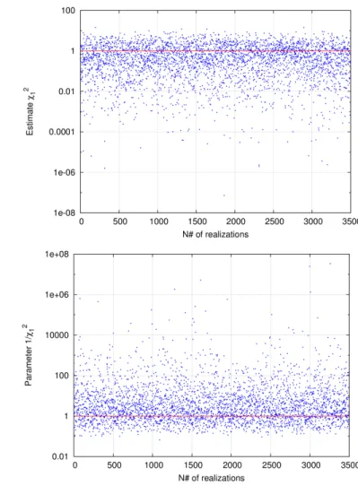
E has the same non negligible value : for example P (σ2 > 10 ˆσE2) = 0.25. However, this probability has completely different consequences in each world.
In the measurement world, the possibly huge values of the true valueσ2 induce the divergence of the a posteriori mean for N < 4 (huge values of 1
χ2 1
in Eq. (20)). These huge values occur in the real world with a non negligible probability and the divergence of the mean is a simple consequence of this existence (see Figure 1(B)).
In the model world for a given true value σ2, the random realizations of the measurements give, with the same non negligible probability, values such that the estimatorσ2
E is much smaller than σ2. In other words, the true unknown value of σ2 is huge, if expressed in units of σˆ2
E, the only available value from the measurements. Unfortunately, these low values ofσˆ2
E with respect to the true value have almost no weight in the estimator expectation given by Eq. (19), and also in the MMSE estimator expectation which is proportional to it: less than 1% of this expectation is due to values of σˆ2
E < 0.1σ2, though the probability of having σˆE2 < 0.1σ2 is the same 0.25 as in the measurement world (see Figure 1(A)).
Because the danger of underestimating the true value is not properly taken into account, the MMSE estimator is a bad estimator for a scale parameter. Though not new (see for example [2]), this statement was often missed [5].
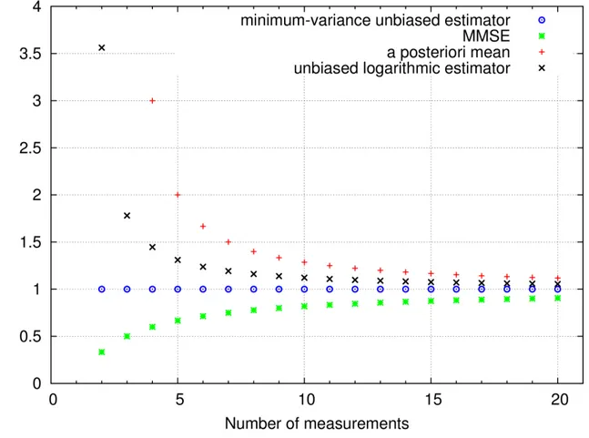
Even for a greater number of measurements, the difference between the estimators remains non negligible. For instance, the MMSE and a posteriori mean differ by 20% for 20 measurements (see Figure 2).
V. SOLUTION: AN OPTIMAL ESTIMATOR ?
The situation of Example 2 seems at first sight desperate, since the “right” estimator in the measurement world diverges. The best solution would be, of course, to make more measurements: E(σ2) is defined for N ≥ 4. In some cases, this is not possible, especially in the time and frequency metrology domain at very long duration (106−107 s): we would have to wait for several days-months. Moreover, appreciable differences remain between the estimators even for more measurements, as shown in Figure 2. The following considerations give clues to the solution:
• A confidence interval on σ2 can be defined without any difficulty: at 95 % of confidence,
σ2 lies between 0.18 ˆσ2
(A)
(B)
Fig. 1. (A): Set of 3500 realizations which follow a χ2
1 distribution. (B): Set of 3500 realizations which follow an inverse χ21
distribution.
of freedom. The divergence of the mean comes from the values above the high limit of this interval.
• Because of this huge confidence interval, only an order of magnitude of σ2 can be
deter-mined, suggesting that the natural variable choice is log(σ2).
• The entire set{di} can be replaced without any loss of information by an estimator, called a sufficient statistics: the three estimators, Eq. (8-10), define each a sufficient statistics for the variance of a gaussian distribution, differing only by a known multiplicative constant for a given number of measurements. More generally,C · ˆσE2 is a sufficient statistics whatever the value of the multiplicative constant C. Likewise the sample mean is a sufficient statistics
Fig. 2. Comparison of the three estimators of Section IV-D, and of the unbiased logarithmic estimator proposed in Section V.
for the determination of the mean of a gaussian distribution. [1]
• To determine the a posteriori law p(θ), we have used the so called “fiducial argument”,
introduced by Fisher [6], which is valid if:
1) no a priori information exists, rendering the measurements strictly not recognizable as appertaining to a subpopulation [6]
2) transformations of a sufficient statistics C · ˆσE2 to u and of θ to τ exist, such that τ is a location parameter for the PDF p(u|τ) [7], i.e. u = log(C · ˆσ2E) and τ = log(θ), transforming (see Eq. (3)) pθ(C · ˆσE2|θ) = pθ
³C·ˆσ2 E θ
´
to pτ(u|τ) = pτ(u − τ).
After this transformation, the quotients characterizing any scaled probability density, Eq. (3), become differences and the probability density in both the model and the measurement worlds can be expressed as a function of u − τ: p(u|τ) = p(τ|u) = f(u − τ), implying a constant a priori probability density π(τ ). Indeed, p(u and τ ) = p(τ |u)p(u) = p(u|τ)π(τ), implying π(τ ) = p(u), where p(u) is constant since u is a constant issued from the measurements.
If such a transformation exists, the derivation of p(θ) is warranted: as stated in Eq. (20), p(σ2|ˆσ2
E) is an inverse χ2 density and the expectation of σ2 can be calculated. On the other hand, the direct use of u and τ , though not yet the most popular choice, allows a perfect symmetry between both worlds [8]. Indeed, for any scale parameter θ we have u = log(ˆθ) + B, τ = log(θ), where B is a constant chosen in order to obtain a non biased estimator in the model world: B such Z +∞ −∞ u · p(u|θ 0)du = Z +∞ −∞ u · f(u − τ 0)du = τ0 (11)
where θ0 is the true value of the parameter θ and τ0 = log(θ0).
Then we have in the measurement world, after measurements leading to a given value u0: Z +∞ −∞ τ · p(τ|u 0)dτ = Z +∞ −∞ τ · f(u 0− τ)dτ = u0. (12)
The demonstration is performed by a variable change x = u − τ0 in Eq. (11), leading to R+∞
−∞ xf (x)dx = 0 by using R+∞
−∞ f (x)dx = 1. Then Eq. (12) is obtained by using y = u0− τ. In the particular case of the Example 2 withN = 2, we find u = log(ˆσ2
E) + B, with B = 1.27. Hence we proposed [8] in linear units a new estimatorσL2 = exp(u) = exp(B)ˆσE2 = 3.56 ˆσ2E. This estimator is log-unbiased: E [log(ˆσ2
L)] = log(σ2) and, in the measurement world E [log(σ2)] = log(ˆσ2
L). In short, log(ˆσ2L) is both an unbiased estimator and an a posteriori mean.
The above arguments extend to other estimators of a scale parameter. The most evident other example is the estimation of the expected lifetimeλ−1of a Poisson process, defined as the inverse
of the mean rateλ. Similar considerations allow the definition of a log unbiased estimator, that is, for example for a unique measurement, 1.78 (i.e. exp(e), where e is the Euler’s constant) times the minimum-variance unbiased estimator. Note that makingN measurements consists in waiting from an origin time t = 0 until the time tN where the Nth event occurs. The minimum-variance unbiased estimator is tN/N . A wrong procedure would be to define a priori a time interval T and to count the number of events in T . Such a procedure induces a priori information on the magnitude of λ and leads to famous absurdities when trying to define unbiased estimators [9].
Let us return to Example 1 under the light of the above considerations. The sample mean ¯d obeys a Gaussian distribution of mean θ and variance σ2/N (for α = 1). Hence, it is directly a location parameter, ensuring that ¯d is both a minimum-variance unbiased estimator in the model world and the a posteriori mean in the measurement world, if no a priori information on the mean is available. This is a great difference with the situation of Eq. (7), where the a priori information, i.e. the a priori mean power E(θ2) of the signal, could be taken into account either with the MMSE estimator or with the a posteriori mean, but not with an unbiased estimator. Note that, in the measurement world, p( ¯d − θ) is no more Gaussian since σ2 is known by its probability density. It is well known that p³√N ( ¯d − θ)/p ˆσ2
E ´
is a Student distribution for ¯d in the model world. Seidenfeld [10], has shown that this law is also, as proposed by Fisher [6], a Bayesian a posteriori law for θ.
Of course, obtaining an unbiased estimator in both worlds is not sufficient to define an optimal estimator. It should also have the minimum variance in the model world. In the measurement world, p(θ) must be constructed from such a minimum-variance unbiased estimator to ensure a minimum variance on θ. In this case, the estimator will be also MMSE because the constant a priori probability density ensures the same MSE in both worlds for a location parameter. For Example 1 in the absence of any a priori information, p(θ) can be inferred either from the sample average or defined as the mean of the probability density equal to the product of the data likelihoods. Both methods lead to the same results, since the sample mean is a complete sufficient statistics for the underlying Gaussian probability. The minimum-variance unbiased estimator can have more complex forms: for example in the case of a biexponential (or Laplace) distribution of the data, it is obtained by adequate weighting of the ordered data [11]. In this case, we have verified that the mean of the product of the data likelihoods gives the same estimator as the so-called “efficient estimator” proposed in [11].
VI. CONCLUSION
We have recalled that the three most popular estimators give very different results for a small number of measurements in some standard situations. If a priori information is available, the difference is irreducible because the best estimator is biased in the direction of this a priori information. If no a priori information is available, except the model of the underlying probability, these three estimators give the same result for a location parameter. For a scale parameter, using the logarithms of the data allows the transformation of this scale parameter to a location parameter, ensuring the equivalence of the three estimators.
VII. AUTHORS
• Eric Lantz ([email protected]) is professor in the Department of Optics,
Femto-ST, at the University of Franche-Comt´e.
• Franc¸ois Vernotte ([email protected]) is professor in the
UTINAM Institute, Observatory THETA, University of Franche-Comt´e.
REFERENCES
[1] G. Saporta, Probabilit´es, analyse des donn´ees et statistique, 3rd ed. Paris: Technip, 2011.
[2] A. Tarantola, Inverse Problem Theory. Elsevier, 1987.
[3] D. Johnson, “Minimum mean squared error estimators,” Connexions, November 2004, http://cnx.org/content/m11267/1.5/.
[4] M. Wahl, Digital Image processing. Boston and London: Artech House, 1987.
[5] S. Kay and Y. C. Eldar, “Rethinking biased estimation,” IEEE Signal Processing Magazine, vol. 25, pp. 133–136, 2008.
[6] R. A. Fisher, Statistical methods and scientific inference, 3rd ed. New York: Hafner, 1973.
[7] D. V. Lindley, “Fiducial distribution and Bayes’ theorem,” Journal of the Royal statistical Society B, vol. 20, pp. 102–107, 1958.
[8] F. Vernotte and E. Lantz, “Statistical biases and very-long-term time stability,” IEEE Transactions on Ultrasonics,
Ferroelectrics and Frequency control, vol. 59, pp. 523–530, 2012.
[9] J. Romano and A. Siegel, Counterexamples in Probability and Statistics. Monterey (CA): Wadsworth & Brooks/Cole, 1986, p. 168.
[10] T. Seidenfeld, “R.A. Fisher’s fiducial argument and Bayes’ theorem,” Statistical Science, vol. 7, pp. 358–368, 1992.
[11] Z. Govindarajulu, “Best linear estimates under symmetric censoring of the parameters of double exponential population,”
ANNEX 1: WIENER FILTERING
Let us construct from the data di = αθ + ni an estimator ˆθ: ˆ θ = βd¯ α = βθ + β N α N X i=1 ni. (13)
Clearly the real coefficient β should approach 1 if the noise term in ˆθ can be neglected, while β should approach 0 if this noise becomes predominant. The mean-square error writes:
E³ ˆθ − θ´2 = (1 − β)2θ2 + µ β N |α| ¶2 N σ2, (14)
where we have used our hypotheses on the noise: ni is centered and additive, i.e. independent of θ, meaning that all cross terms between the true value and the noise vanish. The determination of the value of β minimizing the mean square error is immediate but uses the unknown true value θ:
β = N |α| 2θ2
N |α|2θ2+ σ2. (15)
Hence, to use in practice this filter, we have to replace θ2 by a level of signal E(θ2), known a
priori, leading to Eq. (7). See [4] for more details.
ANNEX 2: DERIVATION OF THEMMSE AND A POSTERIORI MEAN FOR A SCALE PARAMETER
Minimum square error
Following [5], we search a coefficient m relating Eq. (8) and (9): m is defined by ˆσ2 M = (1 − m)ˆσ2
E. Eq. (4) becomes, since σˆ2E is non biased: Eh¡ ˆσ2M − σ2
¢2i
= (m · σ2)2+ (1 − m)2var¡ ˆσ2
E¢ . (16)
Hence the MSE is minimum for ∂m∂ Eh(ˆσ2
M − σ2) 2i = 0: m = var (ˆσ 2 E) var (ˆσ2 E) + σ4 . (17)
Since (N − 1)σˆE2
σ2 obeys a χ2 distribution with (N − 1) degrees of freedom, the variance of ˆσE2 is equal to N2σ−14 , leading to:
1 − m = N − 1N + 1. (18)
A posteriori mean
In the model world, whereσ2 has a definite value, the random variableσˆ2
E can be normalized such that Y = (N − 1)ˆσ2E/σ2 obeys a χ2
N−1 probability densitypY(Y ), of mean N − 1. Let Z = f (Y ) be a random variable which is a monotonic function of Y . If pZ(Z) is the corresponding probability density, we have pY(Y )dY = pZ(Z)dZ, giving immediately for Z = ˆσE2:
E(ˆσE2) = Z ∞ 0 ˆ σE2p(ˆσE2|σ2)dˆσ2E = σ 2 N − 1 E(Y ) = σ2 N − 1 Z ∞ 0 χ2N−1p(χ2N−1)dχ2N−1 = σ2 (19)
In the measurement world, whereσˆ2
E is known, the fiducial argument [6] consists in considering the random variable Z = σ2 = (N − 1)ˆσ2
E/Y , leading to E(σ2) = Z ∞ 0 σ2p(σ2|ˆσE2)dσ2 = (N − 1)ˆσ2E Z ∞ 0 1 χ2 N−1 p(χ2N−1)dχ2N−1. (20)
This quantity is infinite for N < 4 and equal to (N −1)ˆσ2E
N−3 for N ≥ 4. Note that Eq.(20) can be also obtained from a pure Bayesian point of view by introducing an a priori law 1/σ2 to calculate the a posteriori law p(σ2|ˆσ2