HAL Id: hal-00944665
https://hal-enpc.archives-ouvertes.fr/hal-00944665
Submitted on 11 May 2014HAL is a multi-disciplinary open access archive for the deposit and dissemination of sci-entific research documents, whether they are pub-lished or not. The documents may come from teaching and research institutions in France or abroad, or from public or private research centers.
L’archive ouverte pluridisciplinaire HAL, est destinée au dépôt et à la diffusion de documents scientifiques de niveau recherche, publiés ou non, émanant des établissements d’enseignement et de recherche français ou étrangers, des laboratoires publics ou privés.
National corridors for climate change mitigation:
managing industrial CO2 emissions in France
Jeff Bielicki, Guillaume Calas, Richard Middleton, Minh Ha-Duong
To cite this version:
Jeff Bielicki, Guillaume Calas, Richard Middleton, Minh Ha-Duong. National corridors for climate change mitigation: managing industrial CO2 emissions in France. Greenhouse Gases: Science and Technology, 2014, 3 (4), pp.262-277. �10.1002/ghg.1395�. �hal-00944665�
Article published Greenhouse Gases: Science and Technology DOI: 10.1002/ghg.1395
National Corridors for Climate Change
Mitigation: Managing Industrial CO
2 Emissionsin France
Jeffrey M. Bielickia,b,*, Guillaume Calasc,e , Richard S. Middletond, Minh Ha-Duongc
First online: 12 DEC 2013
aDepartment of Civil, Environmental, and Geodetic Engineering, The Ohio State
University, 483b Hitchcock Hall, 2070 Neil Avenue, Columbus, OH 43210, U.S.A.
bThe John Glenn School of Public Affairs, The Ohio State University, 250c Page Hall,
1810 College Road, Columbus, OH 43210. U.S.A.
cCentre International de Recherche sur l’Environnement et le Développement, CNRS,
Campus du Jardin Tropical, 45 bis, avenue de la Belle Gabrielle, 94736 Nogent-sur-Marne Cedex, France.
dEarth and Environmental Sciences, Los Alamos National Laboratory, MS T003, Los
Alamos, NM 87545, U.S.A.
ePresent Address: Calera Corporation, 100A Albright Way, Los Gatos, CA, 95032, U.S.A.
*Corresponding Author: bielicki.2@osu.edu; phone: (614) 688-2131; fax (614) 292-3780.
Keywords: CO2 Capture and Storage; Industrial CO2; Pipeline Routes; Social and
Political Acceptance; Qualitative Scenarios; Optimization
Abstract
Planning for the deployment of carbon dioxide capture and storage (CCS) infrastructure must consider numerous uncertainties regarding where and how much CO2 is produced and where captured CO2 can be geologically
stored. We used SimCCS engineering-economic geospatial optimization models to determine the characteristics of CCS deployment in France and corridors for pipelines that are robust to a priori uncertainty in CO2
production from industrial sources and CO2 storage locations. We found a
number of stable routes that are robust to these uncertainties, and thus can provide early options for pipeline planning and rights-of-way acquisition.
1 Introduction
The need to reduce greenhouse gas (GHG) emissions by present energy systems and industrial systems is well established for environmental, social, economic, and health reasons.1, 2 Carbon dioxide (CO
2) is the most worrisome GHG because of its long
residence time in the atmosphere and the present societal reliance on energy and industrial processes that emit it. A transition away from systems that vent CO2 emissions
to the atmosphere requires the deployment of numerous technologies, many of which are mature enough to be readily deployed.3
Much effort has focused on reducing CO2 emissions from electric power plants that
emit CO2 as a consequence of combusting fossil fuels (namely coal, but also natural gas
and oil). In 2010, fossil-fueled electric power plants contributed approximately 41% of worldwide CO2 emissions.4 In addition,
many industrial facilities also emit CO2 as a byproduct of the conversion processes
that produce their marketable goods. High CO2-emitting facilities include cement
manufacturers, oil and ethanol refineries, ammonia producers, and iron and steel mills, among others. For example, cement manufacturing emitted approximately 1.9 GtCO2 in
2006, and accounts for approximately 5% of anthropogenic CO2 emissions,5 whereas
steel production emitted approximately 2.7 GtCO2 in 2011.6
CO2 capture and storage (CCS) is one technological option that reduces CO2
emissions.3, 7 CCS is an important component of the portfolio of climate mitigation
technologies, in part because it is the only technology that can address CO2 emissions
from across sectors of the economy. CCS is a process whereby CO2 is collected from
large point sources, compressed and transported (most likely by pipeline) to locations where it is injected into deep sedimentary basins. CO2 emissions from industrial sources
may be substantial, and, in contrast to energy sources, may be better located relative to prospective basins for CO2 storage. These candidate storage basins have contained fluids
such as oil, natural gas, and unusable brine for millions of years, suggesting that the CO2
will likely be contained and isolated from the atmosphere. Mechanisms that trap CO2 in
these reservoirs can be classified into four categories7: (1) structural trapping, (2) residual
trapping, (3) solubility trapping, and (4) mineral trapping. The dominant trapping mechanism may evolve over time7 and vary by the type of reservoir; long-term trapping
in saline aquifers may be dominated by structural8 or residual9 mechanisms whereas
solubility mechanisms dominate in oil9 and gas10 reservoirs.
In some quarters, the focus of CO2 management has turned to how CO2 may be put to
beneficial reuse in order to have a business case for CCS activities, and CCS thus been re-branded as CCUS to emphasize the possibility of “U”tilizing CO2. Large volumes of
CO2 may be used to enhance oil recovery (CO2-EOR)11 or natural gas recovery12 and
industrial scale experience with CO2-EOR, and the ability to put CO2 for uses such as
these has been the focus of much effort to develop the requisite knowledge.14 CO
2 that is
captured from anthropogenic sources is sometimes called "byproduct CO2" as opposed to
"extracted CO2" that is mined from natural deposits such as salt domes.15 Other potential
options to use the large volumes of byproduct CO2 include pressure support for
geothermal energy production from hydrothermal sources,16 use as the fluid to stimulate
impervious formations capable of producing electricity from geothermal heat17 and as the
primary working fluid in geothermal energy applications in sedimentary basins.18
A transition away from CO2-emitting economies requires policy, planning, and
regulatory treatment that encourages adoption, and societal acceptance of the associated activities in order for these new means diffuse broadly. Political and institutional commitments to CO2 emissions reduction can occur through a variety of means, including
quotas that cap the amount of CO2 that can be emitted and pricing mechanisms that make
it more costly for a facility to emit CO2. Norway was the first country to enact a CO2 tax,
in 1991, which then led to the first industrial scale CO2-injection-for-storage project at
Sleipner, in 1996. A few places worldwide have followed with mechanisms that impose costs on facilities that emit CO2 to the atmosphere: the European Union Exchange
Trading System (EU-ETS), the Australian Carbon Tax, the Regional Greenhouse Gas Initiative (RGGI) in the U.S. Northeast, the Chicago Climate Exchange, and the California Cap-and-Trade program. In addition, CCS infrastructure planning and deployment must consider a variety of interacting factors. For example, CO2 pipeline
infrastructure must be deployed in a way that is most acceptable and minimally disruptive while designed to connect locations that will be useful over time, given the possible evolution in CO2 emissions locations and quantities as well as the availability of CO2
disposal options for reuse or storage. Originally implemented in 2005, the EU-ETS provided CO2 emissions allowances to six GHG intensive industries: electricity
generation, cement manufacturing, glass production, iron production, chemicals production, and paper and pulp production. After the collapse of permit trading prices in 2007, the EU-ETS was re-designed and broadened for Phase III, from 2013 to 2020. Of importance for this paper, Phase III of the EU-ETS consolidates the 27 individual CO2
emissions caps for each of the member countries into one EU-wide cap, and broadens its application beyond the original six industries; Facilities from industrial sectors in Europe must also possess emissions allocations in order to emit CO2 to the atmosphere. Without
political support that considers the realities of the current physical, economic, and social systems, well-intentioned policy and planning will likely have limited success.
We investigated the desirable spatial arrangement of CCS activities in France, arising from three scenarios for the availability of CO2 disposal options combined with three
scenarios for CO2 emissions from stationary sources. We construct the potential storage
options from a 2011 roadmap for CCS by the French Environment and Energy Agency, Agence de l'Environnement et de la Maîtrise de l'Energie (ADEME)19 that includes
qualitative descriptions of the extent of CCS deployment as a consequence of technical, societal, and regulatory enablers. The CO2 production scenarios are based on data for
CO2 emissions from sources in the electricity and industrial sectors of France from 2003
to 2011 and are constructed a priori uncertainty in the locations and quantities of CO2 We
applied a coupled engineering-economic, geospatial optimization model to the nine combinations of these scenarios to identify the cost-minimized deployment of CCS and the robustness of potential pipeline routes to these differences in CO2 storage availability
and uncertainty in CO2 emissions. France has typically emphasized energy system
planning and public management, but there has been no CO2 transportation pipeline for
private reuse of CO2 to date.
2 Case Study: France
France is an ideal case study for the deployment of CCS for CO2-emitting facilities
from the energy and industrial sectors: (a) France participates in the EU-ETS; (b) the majority of its CO2 emissions come from industrial sources; (c) France has actively
pursued relevant understanding of the technical, social, and political mechanisms and their influence on CCS deployment; and (d) France has typically emphasized energy system planning and public management, but there has been no CO2 transportation
pipeline for private reuse of CO2 to date..
Originally implemented in 2005, the EU-ETS provided CO2 emissions allowances to
six GHG intensive industries: electricity generation, cement manufacturing, glass production, iron production, chemicals production, and paper and pulp production. After the collapse of permit trading prices in 2007, the EU-ETS was re-designed and broadened for Phase III, from 2013 to 2020. Of importance for this paper, Phase III of the EU-ETS consolidates the 27 individual CO2 emissions caps for each of the member countries into
one EU-wide cap, and broadens its application beyond the original six industries; Facilities from industrial sectors in Europe must also possess emissions allocations in order to emit CO2 to the atmosphere.
The amount of CO2 emitted from France between 2003 and 2011 ranged between 131
and 203 MtCO2/year, most of which did not come from the electricity sector. In 2011,
electricity generated in France totaled 530 TWh, 421 TWh (79.4%) of which came from nuclear power plants, 66.5 TWh from renewables (mostly hydroelectric) and 45.1 TWh from facilities that use fossil fuels as the primary source of energy.20 In that year, CO
2
emissions in France totaled 148.3 MtCO2, only one-fifth of which (30.2 MtCO2) came
from facilities with the primary purpose of producing energy.21 As a consequence, France
emitted only 13.9 MtCO2 from the electricity sector in 2011. An equal amount of CO2
was emitted from oil refineries that year, and steel mills emitted 19.5 MtCO2.
Despite having minimal CO2 emissions from the electricity sector and relatively little
remaining coal reserves when compared to other major economies actively pursuing CCS development (e.g., 160 million tonnes vs. 438 billion tonnes in the United States and 40 billion tonnes in Australia)22 France has actively pursued CCS research. For example, the
Lacq Pilot CCS project injected 51,000 tCO2 into a depleted gas reservoir between
January 2010 and March 2013. Overall,
France has three sedimentary basins; the Paris Basin is the largest and includes the Dogger and Trias aquifers as candidate CO2 storage reservoirs. A few studies have sought
to estimate the CO2 storage capacities of these aquifers, one of which estimated that the
Dogger could store 13.6 GtCO2 and that the Trias aquifer could store 15.5 GtCO2.23
In 2010, ADEME developed a CCS roadmap for France through an expert stakeholder-driven scenario process, using well-defined methods.19 The ADEME panel
identified three major topics that will be influential in the development and deployment of CCS: (1) incentives and regulatory policy, more generally, within France, in Europe, and throughout the world; (2) the technical and societal impediments to deployment; and (3) the deployment, maintenance, and operation of the CO2 transportation infrastructure,
including the entities involved with planning and financing this infrastructure. The ADEME study identified four “visions” for the deployment of CCS based on the intersection of two mechanisms underlying the viability of large-scale deployment: the degree to which deployment is impeded by technical and societal restrictions, and the existence of incentives and regulation. The four ADEME Visions are summarized in Table 1.
[Table 1 approximately here]
We used two versions of the Scalable Infrastructure Model for CO2 Capture and
Storage, SimCCS, a geospatial economic-engineering optimization model, that simultaneously considers CO2 capture, transportation, and storage. SimCCSCAP 24, 25
deploys spatially optimized infrastructure based on a quantity target, whereas
SimCCSPRICE 26, 27 deploys the optimal spatial configuration in response to a CO
2 price.
SimCCSPRICE thus considers the costs of the CCS system to be deployed and the costs
incurred by paying the CO2 price for emitting CO2 to the atmosphere. Section 3 provides
more details on the SimCCS models.
We limited our analysis to CO2 capture and transportation within France, leaving the
possibility of international pipelines for future work. Other analyses of infrastructure for CCS in Europe have investigated potential national28 and international29, 30 pipeline
networks. These analyses, however, have not been based on roadmaps that incorporate non-technical constraints on deployment. Further, unlike SimCCS, these methodologies do not have the spatial resolution to incorporate characteristics of the land and surface interests that will influence routing.
[Table 2 approximately here]
Our storage scenarios are based on the scenarios developed by the ADEME process for the interaction between varying degrees of (a) regulation and incentives and (b) technological and societal constraints. We developed three scenarios for CO2 storage
options (Table 2), conforming to the potentials articulated in Visions 2-4 of the ADEME CCUS roadmap for France:
A. North Sea. CO2 captured from French sources is transported by surface
pipelines to a hub in northern France at Le Havre. This CO2 is then transported in
a subsea pipeline to a larger hub at Rotterdam where it is further transported for injection into locations under the North Sea, either for storage or CO2-EOR. Since
Le Havre serves as a hub for further transportation to other offshore locations, there is no capacity constraint.
B. North Sea and Onshore in the Parisian Basin. In addition to the hub at
Le Havre, CO2 could be transported onshore to locations atop the Parisian Basin.
We use effective storage capacities that are less than 10% of previous estimates23:
1.1 GtCO2 in total over our three Trias injection locations and 900 MtCO2 in total
over our three Dogger injection locations. We used the six potential injection locations,31 as shown in Table 3.
C. Offshore. This storage scenario corresponds to Vision 3. In addition to
the hub at Le Havre for CO2 to be stored in the North Sea, a hub is developed in
Southern France at Marseille for offshore storage in the Mediterranean Sea. The Marseille hub, like that at Le Havre, is not modeled with a capacity constraint.
[Table 3 approximately here]
and scaled them using their sensitivity analyses and the parameters for our storage locations. Erreur : source de la référence non trouvée
[Figure 1 approximately here]
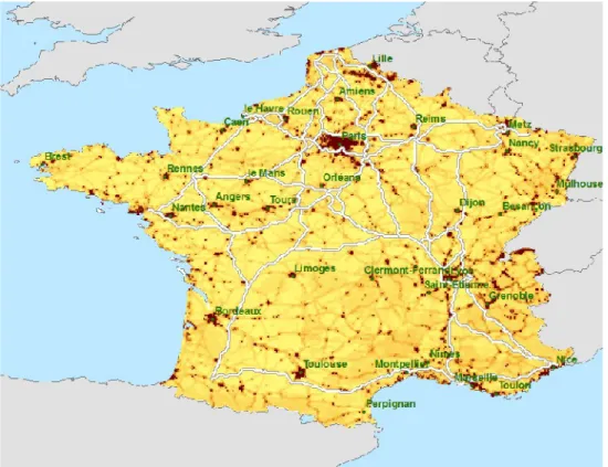
Previous research on CO2 sources in France identified clusters in five industrial areas
that can provide early opportunities for CO2 capture and transportation: Lorraine, lower
Seine, Paris, Nord-Pas-de-Calais, and Provence Alpes-Côte d’Azur.32,33 We acquired CO 2
emissions data for point sources in France from the IREP database 21 for 2003 through
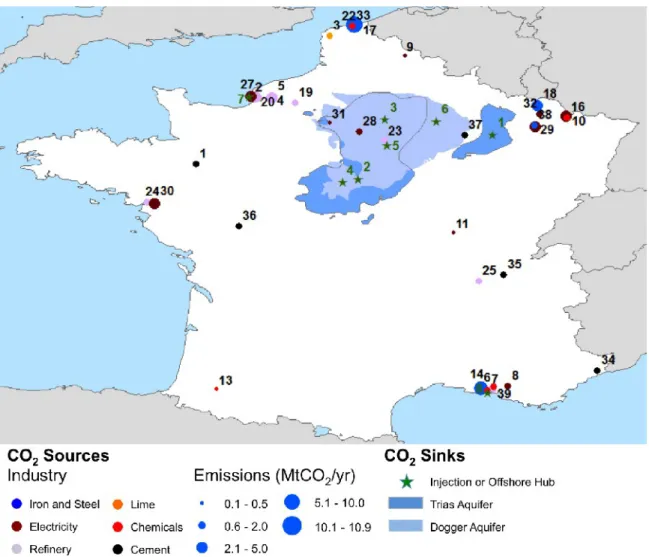
their CO2 emissions at the midpoint (2007) of the data. Figure 1 shows the locations of
these sources and the eight potential CO2 disposal options in Scenarios A-C. For sources,
colors indicate economic sector, and size indicates yearly CO2 emissions capacity. Green
stars indicate the location of sinks in the Parisian Basin or hub locations for offshore pipelines to the North Sea (ID 7) or the Mediterrean Sea (ID 8).
[Table 4 approximately here] [Figure 2 approximately here]
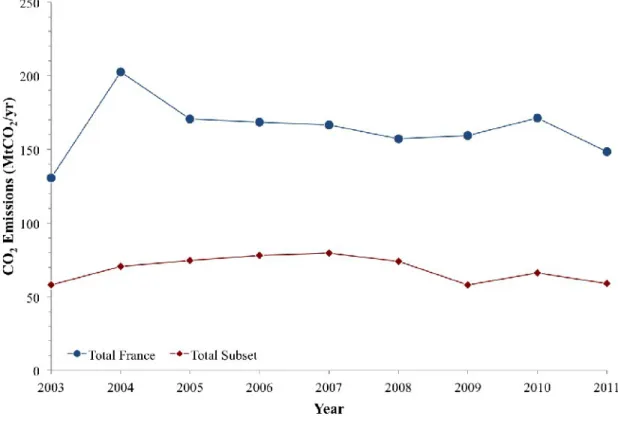
Figure 2 shows the total CO2 emissions from all of the 1,577 sources in the IREP
database for France and from the 39 sources that were selected for this study. Between 2003 and 2011, France averaged emissions of 164 MtCO2/yr; the amount of CO2 emitted
from these 39 sources varied over time (Figure 3), and accounted for between 35% and 48% of the total CO2 emissions in France. In this subset of the data, sources in the
electricity sector emitted 13.9 MtCO2, an equal amount of CO2 was emitted from oil
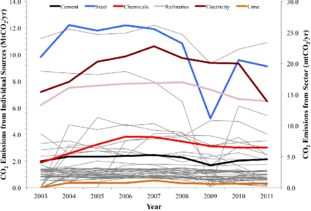
refineries that year, and steel mills emitted 19.5 MtCO2. Some sources did not exist at the
beginning of the time period we used (2003), and some did not exist at the end of the time period (2011). Further, the 2009 global recession is evident in the decrease in industrial output and CO2 emissions; some sources’ CO2 emissions dipped to near zero.
[Figure 3 approximately here]
We constructed three scenarios for CO2 production based on these data for these 39
sources during the time span of this data. These scenarios were established to represent uncertainty in future CO2 production for each individual facility: (1) average, (2)
maximum, and (3) minimum. The minimum scenario, thus assigns zero to those facilities that did not emit CO2 during the timespan, either because they were temporarily or
permanently not operating. We used SimCCS to determine how much of the CO2 that is
produced by each facility in each scenario should be captured, and thus how much would be left to be emitted.
3 The Scalable Infrastructure Model for CO2 Capture and Storage
(SimCCS)
SimCCS, is a coupled engineering-economic geospatial optimization model that
determines the cost-minimized optimal deployment of the integrated CO2 capture,
transport, and storage system.24 SimCCS has been used to model CCS deployment in
California according to a cap on CO2 emissions,24 and extended to model responses to a
infrastructure. SimCCS has also been applied to a range of CO2 emission sources
including coal and natural gas power plants,35 oil shale industry,36 oil sands production,27
and ethylene manufacturing.25 The SimCCS approach has been the point of departure for
other CCS infrastructure models30 and for wind37 and hydrogen38 energy technology
deployment.
SimCCS includes a range of economic and engineering considerations. Capture costs
are separated into capital, fixed operation and maintenance (O&M), and variable O&M costs. Consequently, the model can capture the tradeoff between infrastructure capacity and capture utilization rates. Transportation costs are based on a combination of right-of-way costs and construction costs, including materials, labor, and planning costs. Pipeline costs vary significantly with pipeline capacity. SimCCS splits storage and injection costs into two parts: upfront reservoir costs (such as surveying and permitting) and injection costs. Injection cost for an individual reservoir is driven by the number and cost of wells required to inject the optimized amount of CO2. Each well has a fixed cost (such as the
drilling and material costs) and a variable O&M cost (such as pumping, tracers, and pore space purchase). Each reservoir has a fixed storage capacity and a maximum injection rate. Overall, SimCCS optimizes the infrastructure in order to minimize total costs while (i) capturing a target (or cap) amount of CO2, or (ii) maximizing captured CO2 while
keeping CCS costs below the CO2 price. Since leakage in the system is assumed to be
zero, that amount of CO2 captured by a SimCCS cost-minimizing optimization equals the
amount stored in the geologic reservoir.
We used established cost estimates for CO2 storage in Europe from the Zero
Emissions Platform (ZEP)39 and scaled them using their sensitivity analyses and the
parameters for our storage locations. The ZEP approach establishes broad “most likely”, “maximum”, and “minimum” values for relevant storage parameters, and uses them to estimate storage costs. For generic onshore saline aquifer storage with no legacy wells that can be reworked for CO2 injection for storage, the “most likely” field capacity is 66
MtCO2, which ranges between 40 and 200 MtCO2. The “most likely” well injection rate
is 0.8 MtCO2/year per well, ranging between 0.2 and 2.5 MtCO2/yr. And the “most
likely” well depth is 2000 m, ranging between 1000 and 3000 m. We used three parameters to adjust the ZEP results by the parameters from our injection locations: field capacity, well injection rate, and well depth. We base our cost estimates on a conservatively lower well injection rate of 0.4 MtCO2/year, and use the depths and
estimated capacities specific to our storage options (Erreur : source de la référence non trouvée) to estimate CO2 storage costs for this study.
We used CO2 capture costs from available literature, but considerably less effort has
investigated the cost to capture CO2 from industrial sources than from coal-fired power
plants. We used published studies and publicly available reports31, 40, 41, 42 that provided
estimates of capture costs, including the assumption of 90% capture efficiency. In some cases the literature provided ranges of estimates. Estimating the cost to capture CO2 from
the individual plant. Each facility will have its own characteristics, and detailed studies such as these, while important for the management, operation, and decision-making of any specific plant, are beyond the scope of this paper. For our simulations, we chose realistic representative capture costs for each facility according to its industrial sector (Table 4).
[Table 4 approximately here]
The map used by SimCCS to identify potential routes for CO2 pipelines incorporates
various aspects of the physical, social, and cultural topography that are combined to produce a “cost surface”. This cost surface indicates the degree to which pipeline infrastructure should avoid that location.37 We used the cost surface developed for
France,31 which includes routing considerations to avoid:
• Existing infrastructure, including roads, highways, and railroads
• Existing rights-of-way, including existing pipelines and transmission lines
• Nature reserves, including biological, biosphere, and nature reserves
• Elevation changes (slope and aspect)
• National and regional parks
• Special protected areas
• Population density
SimCCS applies a modified version of Dijkstra’s shortest path algorithm to the cost
surface in order to determine potential pipeline routes between all combinations of sources and sinks (grey in Figure 4). These potential routes thus avoid, to the extent possible, places where it may be more costly to build pipelines.
[Figure 4 approximately here]
Since energy is required to operate capture, compression, and pumping equipment throughout the CCS supply chain, these “energy penalties” can result in additional CO2
emit CO2. If this additional CO2 is not captured, and instead emitted to the atmosphere,
the net change in CO2 emissions to the atmosphere will be less than the amount of CO2
being captured and stored. Quantifying the CO2 emissions that are avoided requires an
assessment of where and how the extra energy is being produced. If the electricity comes from a coal-fired power plant, for example, there will be extra CO2 emissions. But if the
electricity for the energy penalty is produced by a nuclear power plant, there will not be any additional CO2 emissions and the CO2 that is captured and stored will equal the
avoided CO2. Methods have been developed to incorporate avoided CO2 into pipeline
planning43, but our analysis focused on the CO
2 captured by the sources we include in our
three CO2 production scenarios and stored in the three sink availability scenarios. We did
not model electricity sources and flows or the internal characteristics of a power plant that may provide its own makeup electricity to satisfy the energy penalties, and thus we did not attempt to quantify the extra CO2 that could be emitted as a result of the energy
penalties incurred by infrastructure SimCCS deploys. As a consequence, we implicitly assumed that the electricity for the energy penalties comes from elsewhere in the economy, but we do not allocate that electricity to specific sources and thus we cannot quantify the difference between the amount of CO2 that is captured and stored and the net
amount of CO2 emitted to the atmosphere.
4 Results and Discussion
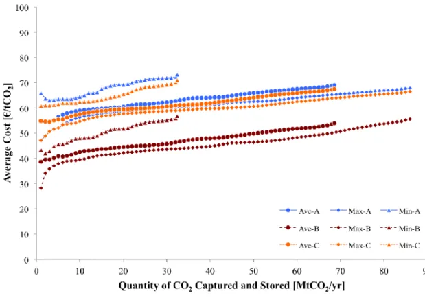
Figure 5 shows the average costs of the CCS system for all of the nine combinations of the three CO2 production quantities and the three storage options as a function of the
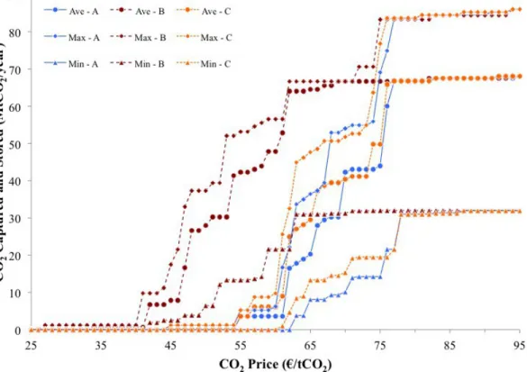
amount of CO2 captured and stored. Figure 6 shows the amount of CO2 captured and
stored as a function of the CO2 price for these nine combinations. This figure corresponds
to the marginal costs associated with Figure 5, with the axes switched. Holding the storage options constant, scenarios involving the minimum amount of CO2 production are
always more costly than those with the average amount of CO2 over the timeline, and
these average CO2 production scenarios are, in turn, more costly than scenarios that
consider the maximum amount of CO2.
[Figure 5 approximately here]
[Figure 6 approximately here]
Average system costs decrease as the number of storage options increase because additional storage options may be cheaper and/or located closer to the CO2 sources,
resulting in a possible decrease in storage and/or transportation costs. If these additional storage options are not cost-effective to deploy, the economies of scale that can occur
when pipelines are networked together to combine CO2 flows into larger diameter
pipelines are unchanged. As a consequence, holding the CO2 sources constant while
increasing the options for CO2 disposal can only reduce average costs.44 In the
application here, systems with storage scenario A (offshore hub at Le Havre) are more costly than those with storage scenario C (offshore hubs at Le Havre and Marseille). Storage scenario B, where CO2 can be transported to Le Havre for storage under the
North Sea or to locations within the Parisian Basin, is the cheapest scenario. Single point-to-point pipelines are inefficient at the system level, and having a few larger sinks can reduce costs through economies of scale. But somewhere between these two end cases, arrangements can exist that might minimize costs due to the flexibility of storage options.
Marginal costs are critical for understanding when a particular source could begin to cost-effectively capture CO2. A CO2 price of €65/tCO2, for example, means that
SimCCSPRICE optimally identifies the combination of sources, pipelines, and sinks
whereby the amount of managed CO2 is maximized while ensuring that the system-wide
marginal cost is less than €65/tCO2. That is, when making the CCS system handle one
more unit of CO2, that unit of CO2 will cost €65/tCO2 or more.
Some differences exist between the results for storage scenario A (Le Havre) and storage scenario C (Le Havre and Marseille) within a single CO2 production scenario.
Both of these storage scenarios transport CO2 for offshore storage; the availability of
these hubs is the major difference between the two scenarios. Adding the hub at Marseille expands the disposal options, which can reduce the CO2 price at which CCS is
cost-effective because the system-wide costs may be reduced as a result of building a shorter pipeline or deploying slightly more costly sources that are more proximal to the additional storage option. The lower-cost network, due to increased storage options, can facilitate more CO2 being captured and stored for any given CO2 price.
The plateaus in Figure 6 arise because the majority of the CO2 being produced by the
sources is captured and stored in systems with lower CO2 prices. When the minimum
CO2 production is considered, CCS begins to be deployed at €61/tCO2 (Scenario C) and
€63/tCO2 (Scenario A), but deployment begins at the same CO2 price for the average and
maximum CO2 production scenarios: 55 €/tCO2 and 45 €/tCO2, respectively. While CCS
begins to be deployed at the same CO2 price in this maximum CO2 scenario, the rest of
the curve for the amount of CO2 being captured is shifted to the left and system-wide
cost-savings can be realized.
[Figure 7 approximately here]
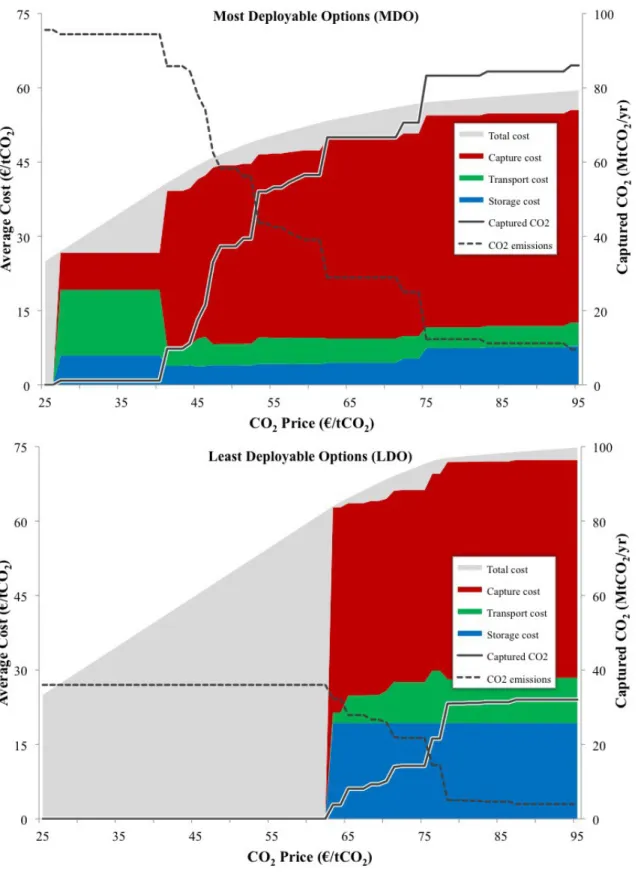
Figure 7 shows the breakdown in costs for the two cases at each end of the spectrum of CO2 production and storage options. The top image shows the characteristics of the
most optimistic system—the Most Deployable Options (MDO)—where the maximum amount of CO2 production is considered along with the most storage options (Scenario
B). The bottom image shows the characteristics of the most pessimistic system—the Least Deployable Options (LDO)—where the minimum amount of CO2 production is
considered with only one offshore storage option (Scenario A). These stacked area graphs show the costs for CO2 capture (red), transport (green), and storage (blue). The grey area
represents the system-wide CCS cost which includes the CO2 price applied to any
emissions. When the capture cost (i.e., stacked blue, green, and red areas) and CO2 price
are identical, the stacked areas and the grey area cost coincide. Solid lines indicate how much CO2 is captured and dashed lines indicate how much CO2 is emitted.
As stated above, the optimal systems deployed by SimCCS are built “all at once” at a constant CO2 price. The results in Figure 7 show that much more CO2 is captured, at
lower CO2 prices, and at lower average costs, for the MDO than for the LDO. A single
CO2 source—a lime manufacturer—captures 1.2 MtCO2/yr for systems designed for CO2
emissions prices from €27/tCO2 to €41/tCO2. CCS systems designed for a €41/tCO2 price
capture an additional 8.4 MtCO2/yr from three electricity-generating sources. The amount
of CO2 captured then climbs relatively steadily for systems designed for CO2 prices up to
€75/tCO2 until flattening again at 83 MtCO2/yr. In contrast, in the LDO case, CO2 is first
captured for systems designed for a CO2 price of €63/tCO2 when the system manages 3.8
MtCO2/yr; for systems designed for CO2 prices above €63/tCO2 the amount captured
increases relatively steadily to until a system designed for €78/tCO2 captures 31
MtCO2/yr.
For the LDO case, CO2 capture flattens when 5 tCO2/yr of capturable CO2 are not
captured, and are thus emitted to the atmosphere at a €78/tCO2 price. In contrast, more
than twice this amount (12.3 tCO2/yr) of capturable CO2 is emitted in the MDO case
when the capture curve flattens. While more CO2 is emitted (i.e., not captured) at the
high end of the CO2 prices, much more CO2 is captured in the MDO than in the LDO: 83
MtCO2/yr for MDO vs. 32 tCO2/yr for LDO. In addition, the average of total system
costs, including both CCS infrastructure costs and costs incurred from emitting CO2 (CO2
emissions x CO2 price), is 15-20% less for the MDO system than the LDO system.
[Figure 8 approximately here]
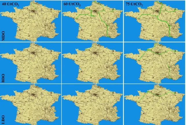
Figure 8 shows the spatial deployment of the integrated CCS system for CO2 prices of
€40/tCO2, €60/tCO2, and €75/tCO2 for the MDO (top row), LDO (bottom row), and a
scenario between MDO and LDO (middle row) combinations. The "between combination" (BDO) is the average amount of CO2 production combined with the two
offshore storage options. Green lines in Figure 8 indicate where pipelines are deployed on the potential routes (grey). Only the MDO has CO2 captured at €40/tCO2 price, where the
one lime manufacturer in northern France captures and transports its CO2 for injection
into one of the Trias injection locations in the Parisian Basin. This system expands substantially by €60/tCO2, where an integrated network captures CO2 from 32 sources
and transports that CO2 to five storage locations, all of which are located onshore. This
network is more extensive at €75/tCO2, as it connects all but three of the costliest and
smallest sources with the onshore reservoirs.
In contrast, a system designed for €60/tCO2 for the BDO case will deploy only three
sources close to the offshore hubs. By €75/tCO2, CO2 is captured from all but eight of the
sources and is transported by four single (not networked) pipelines, to the offshore hubs, three of which terminate at Le Havre. The pipelines extend from near Nantes (in the west), along the northern coast to near Lille (in the North), and near Metz (in the East) to the northern offshore hub at Le Havre, and from just north of Saint Etienne south to the offshore hub on the Mediterranean Sea at Marseille. The LDO deploys two of these routes at €75/tCO2: the routes from near Nantes to Le Havre and near Metz to Le Havre.
[Figure 9 approximately here]
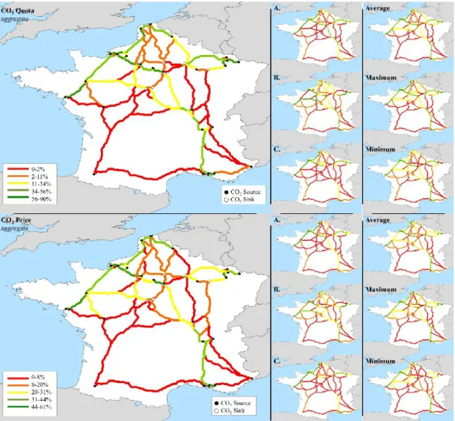
Altogether, Figure 9 shows the relative frequencies by which potential pipeline routes are chosen across all nine combinations of CO2 production and storage options—for
1,203 optimizations conducted by two models of the geospatial deployment of CCS infrastructure, one that optimizes based on the least cost solution to a CO2 quota (Figure
9, top row) and one that optimizes based on the least cost solution to a CO2 price (Figure
9, bottom row). In Figure 9, pipeline routes are color-coded by the quintile in which they are deployed, for the aggregate results by CO2 production scenario (right), CO2 storage
option (middle), and altogether (left) according to CO2 quotas (top) and CO2 prices
(bottom). . Green indicates that the route was deployed in the top 20% of the time, whereas red indicates that the route was deployed the bottom 20%. The percentages in the legends indicate the percentage of model runs within each quintile. The routes that are deployed most often, and are thus most robust to the emissions and storage
uncertainties, are in the top quintile (shown in green).
Figure 9 can be used to indicate where the priorities for pipeline planning and Rights-of-Way (ROW) acquisition should be focused, given the fluctuations in CO2 emissions
and the a priori uncertainty of CO2 storage options. The route south from Saint Etienne to
Marseille and the routes that extend from Le Havre southwest to near Nantes, northeast to near Lille, and east along a route south of Paris are all in the top quintile of deployed routes. In addition, a segment of this latter east-west route extending from Reims (just east of Paris) west to Metz where two other segments, one from Nancy to the south and one from the east, are also among the most deployed routes.
5 Conclusions
We investigated pathways for CCS deployment in France using the concept of a “corridor” in numerous ways: (a) our storage scenarios were based on a prior expert-elicitation process that developed scenarios based on institutional and social conditions that encourage, to varying degrees, CCS deployment;19 (b) our case study is for a country
where the majority of its large point source CO2 emissions are from the industrial, not
electrical, sector (France); (c) our CO2 production scenarios are based on the
characteristics of eight years of large point source CO2 emissions; and (d) we produced a
map that indicates priorities for pipeline routes based on how robust these routes are to the a priori uncertainty in CO2 production and CO2 storage options.
We constructed options for CO2 storage based on the qualitative scenarios elicited
from experts and used them in combination with three scenarios for CO2 production.
These CO2 production scenarios were based on summary statistics of the emissions by
multiple industrial sources in France between 2003 and 2011. While there was variability in the quantities and locations of CO2 emissions in France over this timeframe, the
application of quantitative modeling to qualitative scenarios demonstrates how approaches that optimize infrastructure deployment can be combined with qualitative scenarios that incorporate various degrees of political and social restrictions to assist planning under a variety of situations and in advance of actual deployment.
Even with uncertainty in how many options there may be in the future and where and how much capturable CO2 may be produced, we found that a number of corridors for
pipelines within France exist across the combinations of scenarios; pipeline routes that are robust to the uncertainty in these parameters exist and may be the focus of advance planning and investment for ROWs.
6 Acknowledgments
This international cooperation was supported in part by ADEME convention 10 94 C0012.
7 Tables and Figures
Table 1: Visions for CCS Deployment in France (ADEME, 2011)
Restrictions due to Technical and Societal Concerns
Strong Weak R es tr ic ti on s d u e to I n ce n ti ve s an d R eg u la to ry P ol ic y S tr on g Vision 1: Incremental deployment of CCS.
Vision 2: Restricted to a few large
sources and sectors that cannot implement other means to reduce CO2
emissions.
W
ea
k Vision 3: Strong pooling of CO2
from multiple sources and storage in offshore reservoirs.
Vision 4: Large-scale CCS deployment with storage in onshore and offshore reservoirs.
As used by ADEME, ‘strong’ restrictions significantly impede deployment, whereas ‘weak’ restrictions impose only minimal barriers.”
Table 2 : Case Studies and Sinks for CO2
Case Study Onshore (IDs) Offshore (IDs)
A. North Sea North Sea (7)
B. North Sea and
Parisian Basin Trias (1-3), Dogger (4-6)
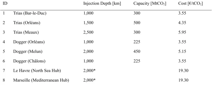
Table 3: CO2 Sink Locations, Reservoirs, and Characteristics
ID Injection Depth [km] Capacity [MtCO2] Cost [€/tCO2]
1 Trias (Bar-le-Duc) 1,000 300 3.55 2 Trias (Orléans) 1,500 500 4.35 3 Trias (Meaux) 2,500 300 5.95 4 Dogger (Orléans) 1,000 225 3.55 5 Dogger (Melun) 2,000 450 5.15 6 Dogger (Châlons) 1,000 225 3.55
7 Le Havre (North Sea Hub) 2,000* 19.30
8 Marseille (Mediterranean Hub) 2,000* 19.30
Unless otherwise noted, injection depths and capacities are from Coussy (2009), BRGM (2009)45, and Calas (2011)
Table 4: Major CO2 Sources and Characteristics in Five Industrial Areas in France
Sector IDs Total Capturable CO2
(MtCO2/yr) CO2 Capture Costs (€/tCO2) Cement 1, 2, 34-37 6.41 48.87 Chemicals 4, 13, 15, 16, 26, 33, 39 8.11 41.35 Electricity 8-11, 27-32 22.77 34.59 Lime 3 1.16 7.52
Iron and Steel 14, 17, 18, 38 25.53 53.38
Refining 5-7, 12, 19-25 16.82 41.35
Figure 1: Carbon Dioxide Sources and Sinks – Sources: Thirty-nine sources and IDs
are shown. Colors indicate economic sector, and size indicates yearly CO2 emissions
capacity. Sinks: Green stars indicate the location of sinks in the Parisian Basin (Trias Aquifer, IDs 1-3, depth 1500-1800m; Dogger Aquifer, IDs 4-6, depth 2000-2500m) or hub locations for offshore pipelines to the North Sea (ID 7) or the Mediterrean Sea (ID 8).
Figure 2: Total CO2 Emissions in France and the Total CO2 Emissions from the 39
Sources Selected in Five Industrial Areas - Over the span of the nine years between
2003 and 2011, France averaged emissions of 164 MtCO2/yr. Over this timespan, CO2
emissions from the 39 sources in this study ranged from 35% and 48% of the total CO2
Figure 3: CO2 Emissions for Each Source (Primary Axis) and by Sector (Secondary
Axis) for the 39 CO2 Sources in France Considered – CO2 emissions by each source
can fluctuate, with some sources having zero emissions at the beginning of the time span, some at the end, and some temporarily fluctuating to almost zero during the time span.
Figure 4: Cost Surface and Candidate Pipeline Network – The cost surface used to
generate the candidate network (grey) indicates the degree to which locations should be avoided when routing CO2 pipeline infrastructure. The candidate network indicates
potential routes that can be chosen to link CO2 sources (black circles) and CO2 sinks
Figure 5: Average Cost Curves for CCS Deployment in all Nine Combinations of
CO2 Production and Storage Options – Blue lines and markers are the results for
storage scenario A, where CO2 is transported to Le Havre as a hub for offshore storage.
Red markers and lines are the results for when injection into the Parisian Basin is available in addition to Le Havre. Orange Markers and lines are the results for offshore storage only—scenario C with hubs at Le Havre and Marseille. Circles indicate the average CO2 production from each source was modeled. Diamonds indicate that the
maximum CO2 production from each source was modeled. Triangles indicate that the
Figure 6: CO2 Capture Curves for Nine Combinations of CO2 Production and
Storage Scenarios – This figure corresponds to the marginal costs associated with Figure
Figure 7: Cost and Performance Characteristics of Integrated CCS Systems for Most Deployable Options (Max – B) and the Least Deployable Options (Min – A)
Combinations of CO2 Production and Storage Scenarios - The stacked area graphs
show the costs for CO2 capture (red), transport (green), and storage (blue). The grey area
emissions. When the capture cost (i.e., stacked blue, green, and red areas) and CO2 price
are identical, the stacked areas and the grey area cost coincide. Solid lines indicate how much CO2 is captured and dashed lines indicate how much CO2 is emitted.
Figure 8: Spatial Deployment of CCS CO2 Pipelines in France for Select CO2 Prices
and Combinations of Deployable Options Based on CO2 Storage Options
Availability and CO2 Production Quantities – The amount of CO2 captured from
sources is shown as the red portion of the pink pie, and the amount of CO2 delivered to a
sink is the blue portion of the light blue pie. Green lines indicate where pipelines are deployed in the potential routes (grey). The top row contains the most promising combination of scenarios (maximum CO2 production and offshore and onshore storage
options) whereas the bottom row contains the least promising combination of scenarios (minimum CO2 production and one offshore storage option).
Figure 9: Corridors for CO2 Pipelines in France Indicating the Percentage of the
Model Runs in which Pipeline Segments were Deployed – Pipeline routes are color-coded by the quintile in which they are deployed, for the aggregate results from the CO2
Quota models (top row) and the CO2 Price models (bottom row). Green indicates that the
route was deployed in the top 20% of the time, whereas red indicates that the route was deployed the bottom 20%. The percentages in the legends indicate the percentage of model runs within each quintile. The smaller images show the results aggregated by storage scenarios A-C (middle columns) and by CO2 production scenarios (right
1 IPCC (2007). “Climate Change 2007: Mitigation. Contribution of Working Group III to the Fourth Assessment Report of the Intergovernmental Panel on Climate Change.” Cambridge University Press: Cambridge, United Kingdom and New York, N.Y. USA.
2 GEA (2012). “Global Energy Assessment - Toward a Sustainable Future.” Cambridge University Press, Cambridge, UK and New York, NY, USA and the International Institute for Applied Systems Analysis, Laxenburg, Austria.
3 Pacala, S. and Socolow, R. (2004). “Stabilization Wedges: Solving the Climate Problem for the Next 50 Years with Current Technologies.” Science, 305, 968-972.
4 IEA (2012). “CO2 Emissions from Fuel Combustion: Highlights.” IEA Statistics, International
Energy Agency. Available at: http://www.iea.org/co2highlights/co2highlights.pdf
5 IEA (2008) “Cement Technology Roadmap: Carbon Emissions Reductions to 2050.”
International Energy Agency. Available at:
http://www.iea.org/publications/freepublications/publication/Cement.pdf
6 WSA (2012). “Sustainable Steel 2012: Policy and Indicators.” World Steel Association. Available at: http://www.worldsteel.org/dms/internetDocumentList/press-release-downloads/2012/Sustainable-Steel-2012/document/Sustainable%20Steel%202012.pdf
7 IPCC (2005). “Special Report on Carbon Dioxide Capture and Storage.” Metz, B., Davidson, O., Coninck, H., Loos, M., and Meyer, J. P., Intergovernmental Panel on Climate Change. Cambridge: Cambridge University Press: 2005; p 431.
8 Johnson, J., and Nitao, J., and Knauss, K. (2004) “Reactive Transport Modelling of CO2 Storage
in Saline Aquifers to Elucidate Fundamental Processes, Trapping Mechanisms, and Sequestration Partitioning.” Geological Society of London Special Publication on Carbon Sequestration Technologies. Lawrence Livermore National Laboratory, UCRL-JRNL-205627.
9 Han, W., McPherson, B., Lichtner, P., and Wang, F. (2010). “Evaluation of Trapping Mechanisms in Geologic CO2 Sequestration: Cast Study of SACROC Norther Platform, a
35-Year CO2 Injection Site”. American Journal of Science, 310, 282-324.
10 Gilfillan, S., Lollar, B., Holland, G., Blagburn, D., Stevens, S., Schoell, M., Cassidy, M., Ding, Z., Zhou, Z., Lacrampe-Couloume, G., and Ballentine, C. (2009). “Solubility trapping in formation water as dominant CO2 sink in natural gas fields.” Nature, 458, 614-618.
11 Bachu, S., Shaw, J., and Pearson, R. (2004). “Estimation of Oil Recovery and CO2 Storage
Capacity in CO2 EOR Incorporating the Effect of Underlying Aquifers.” Society of Petroleum
Engineers, 89340-MS.
12 Oldenburg, C., Stevens, S., and Benson, S. (2004). “Economic Feasibility of Carbon Sequestration with Enhanced Gas Recovery (CSEGR).” Energy, 29(9–10). 1413-1422.
13 White, C., Smith, D., Jones, K., Goodman, A., Jikich, S., LaCount, R., DuBose, S., Ozdemir, E., Morsi, B., and Schroeder, K. (2005). “Sequestration of Carbon Dioxide in Coal with Enhanced Coalbed Methane Recovery: A Review” Energy and Fuels, 19(3), 559-724.
14 NETL (2010). “Storing CO2 and Producing Domestic Crude Oil with Next Generation CO2
-EOR Technology: An Update.” U.S. Department of Energy, National Energy Technology laboratory. DOE/NETL 2010/1417.
15 Middleton, R., Levine, J., Bielicki, J., Rice, M., Viswanathan, H., Carey, J., and Stauffer, P. (2013) Ethylene extracted vs byproduct “Ethylene:CO2-EOR – jumpstarting commercial-scale CO2 capture and storage”. Submitted to Environmental Science & Technology.
16 Buscheck, T., Elliot, T., Celia, M., Chen, M., Sun, Y., Hao, Y., Lu, C., Wolery, T., and Aines, R. (2013). “Integrated Geotherman-CO2 Reservoir Systems: Reducing Carbon Intensity through
17 MIT (2006). “The Future of Geothermal Energy.” Massachusetts Institute of Technology, Cambridge, MA.
18 Randolph, J., and Saar M. (2011). “Combining Geothermal Energy Capture with Geologic Carbon Dioxide Sequestration.” Geophysical Research Letters, (38), L10401.
19 ADEME (2011) Le captage, transport, stockage géologique et la valorisation du CO2. Feuille de route stratégique. Available at: http://www2.ademe.fr/servlet/KBaseShow? catid=24277#thm1tit5
20 EIA (2013). “International Energy Statistics.” U.S. Energy Information Administration, Available at: http://www.eia.gov/cfapps/ipdbproject/iedindex3.cfm
21 IREP (2013). “Registre Francais des Emissions Polluantes.” Ministère de l'Ecologie, du
Développement Durable, et de l'Energie. Available at:
http://www.irep.ecologie.gouv.fr/IREP/index.php
22 EIA (2012). “U.S. Coal Reserves.” U.S. Energy Information Administration. Available at:
http://www.eia.gov/coal/reserves/
23 Bonijoly, D., Ha-Duong, M., Leynet, A., Bonneville, A., Broseta, D., Fradet, A., Le Gallo, Y., Munier, G., Nédelec, B., and Lagneau. V. (2009) “METSTOR: a GIS to look for potential storage zones in France. Energy Procedia, 1(1), 2809-2816.
24 Middleton, R., Bielicki, J., (2009). A scalable infrastructure model for carbon capture and storage: SimCCS. Energy Policy 37, 1052-1060.
25 Middleton, R. (2013) “A new optimization approach to energy network modeling: anthropogenic CO2 capture coupled with enhanced oil recovery.” International Journal of Energy Research. DOI: 10.1002/er.2993
26 Kuby, M., Bielicki, J., Middleton, R., (2011). Optimal Spatial Deployment of CO2 Capture and Storage Given a Price on Carbon. International Regional Science Review 34, 285-305.
27 Middleton, R., Brandt, A., (2013). “Using Infrastructure Optimization to Reduce Greenhouse Gas Emissions from Oil Sands Extraction and Processing.” Environmental Science &
Technology 47, 1735-1744.
28 Klokk, O., Schreiner, P., Pages-Bernaus, A., Tomasgard, A., (2010). Optimizing a CO2 value
chain for the Norwegian Continental Shelf. Energy Policy 38, 6604-6614.
29 Mendelevitch, R., Herold, J., Oei, P.-Y., Tissen, A., (2010). “CO2 Highways for Europe:
Modelling a Carbon Capture, Transport and Storage Infrastructure for Europe.” CEPS Working Document No. 340.
30 Morbee, J., Serpa, J., Tzimas, E., (2012). “Optimised deployment of a European CO2 transport
network.” International Journal of Greenhouse Gas Control 7, 48-61.
31 Calas, G. (2011). “Le transport de dioxyde de carbone par canalization: Modalités de développement et modélisation en France des réseaux de transport dans le cadre du captage et stockage de CO2.” Mémoire de Master 2 Recherche, Économie du Développement Durable, de
l’Environnement et de l’Énergie
32 Ha-Duong, M. (2009) “SOCECO2. Économie et sociologie de la filière capture et stockage géologique du CO2. Poster at the ANR symposium “Quelle recherche pour les énergies du futur?” November 19-20, 2009. Available at: http://minh.haduong.com/files/AfficheSOCECO2-2552x3402.png
33 Coussy, P. (2009). “French CC Roadmap: SocECO2 Project Scenarios”. Communication to the
Recent advances in CCS economics and sociology workshop, Pau, France, 9-10 April 2009. Available at: http://www.centre-cired.fr/IMG/pdf/Coussy-2009-SOCECO2Scenarios.pdf
34 35 36 37 38
39 ZEP (2011). “The Costs of CO2 Storage: Post-demonstration CCS in the EU”. European
Technology Platform for Zero Emission Fossil Fuel Power Plants. Available at:
http://www.zeroemissionsplatform.eu/library/publication/168-zep-cost-report-storage.html
40 GCCSI (2012) “The Global Status of CCS: 2012”. Global CCS Institute. Canberra, Australia. Available at: http://www.globalccsinstitute.com/publications/global-status-ccs-2012.
41 UNIDO (2010). “Carbon Capture and Storage in Industrial Applications.” United Nations
Industrial Development Organization. Technology Synthesis Report. Working Paper –
November 2010. Available at:
http://www.unido.org/fileadmin/user_media/Services/Energy_and_Climate_Change/Energy_Eff iciency/CCS_%20industry_%20synthesis_final.pdf
42 IEA (2011). “Technology Roadmap: Carbon Capture and Storage in Industrial Applications.”
International Energy Agency and United Nations Industrial Development Organization.
Available at:
http://www.unido.org/fileadmin/user_media/Services/Energy_and_Climate_Change/Energy_Eff iciency/CCS/CCS_Industry_Roadmap_WEB.pdf
43 Fimbres Weihs, G., and Wiley, D. (2012). “Steady-State Design of CO2 Pipeline Networks for
Minimal Cost Per Tonne of CO2 Avoided.” International Journal of Greenhouse Gas Control, 8,
150-168.
44 Bielicki. J. (2009). Integrated Systems Analysis and Technological Findings for Carbon Capture and Storage Technology Deployment. Ph.D. Dissertation. Harvard University.
45 BRGM (2009). “SOCECO2 - Evaluation technico-économique et environnementale de la fili`re captage, transport, stockage du CO2 à l’horizon 2050 en France.” Final Report: BRGM/RP-57036-FR. Available at: http://www.centrecired.fr/IMG/pdf/06-BRGM-57036-SOCECO2-EvaluationTechnicoEconomiqueEtEnvironnementale.pdf