Analysis of two- and three-dimensional flow separation

Analysis of Two- and Three-dimensional Flow Separation

by

Olivier Grunberg

B.S. in Mathematics, University of Paris VII, France (2000) M.S. in Fundamental Sciences, Ecole Polytechnique, France (2002)

Submitted to the Department of Mechanical Engineering in partial fulfillment of the requirements for the degree of

Master of Science in Mechanical Engineering

at the

MASSACHUSETTS INSTITUTE OF TECHNOLOGY

February 2004

©

2004 Massachusetts Institute of Technology. All rights reserved.

Signature of Author ... Departmept of MecAan C ertified by ... A ccepted by ...

if

ical Engineering December 19, 2003 /,I A",

...

George Haller Associate Professor mhesis Supervisor Ain A. Sonin Professor of Mechanical Engineering Chairman, Department Committee on Graduate Students

MASSACHUSETTS INS E

OF TECHNOLOGY

JE

l

2 0

20041

LIBRARIES

Analysis of Two- and Three-dimensional Flow Separation by

Olivier Grunberg

Submitted to the Department of Mechanical Engineering on December 19, 2003, in partial fulfillment of the

requirements for the degree of

Master of Science in Mechanical Engineering Abstract

Prandtl (1904) showed that streamlines in a steady flow past a two-dimensional streamlined body separate from the boundary where the skin friction (or wall shear) vanishes and admits a negative gradient. Although commonly thought otherwise, these separation conditions are purely kinematic: They can be derived for any two-dimensional steady vector field that con-serves mass (see, e.g. Shariff, Pulliam, and Ottino 1991).

Haller (2002) managed to extend the Lagrangian separation theory to compressible two-dimensional velocity fields with general time dependence. Specifically, he defines unsteady flow separation as a material instability induced by an unstable manifold of a distinguished boundary point. In this general context, the unstable manifold is a time-dependent material line that shrinks to the separation point in backward time. In forward time, the unstable manifold attracts and ejects particles from a vicinity of the boundary.

Using the above Lagrangian definition, the above kinematic separation theory renders math-ematically exact Eulerian criteria for the location of time-dependent unstable manifolds. The theory only assumes local mass conservation and regularity for the unsteady velocity field.

After recalling the main points of Haller's theory, we apply it to a specific model: a two-dimensional pitching airfoil. We first analyze the flow around the airfoil, and show how, under certain conditions, separation happens on the upper part of this airfoil. Next we consider the unsteady flow conditions, and determine the shape of the separation profile emanating from the wing. At that point, we also outline a new approach to the control of separation.

In the second part of this thesis, we extend Haller's two-dimensional separation theory to three-dimensional flows, treating the case of open and closed separation separately.

Next, we use a method developed by Perry and Chong (1986) to derive expansions of the Navier-Stokes equations that we use as models of three-dimensional separation. We verify our theory on those models.

Finally we discuss new results on genuinely three-dimensional aspects of flow separation: open and closed separation, separation lines and separation surfaces.

Thesis Supervisor: George Haller Title: Associate Professor

Acknowledgements

First and foremost, I would like to express my sincere and deep gratitude to my advisor, Professor George Haller, for his guidance, advice and encouragement throughout the course of this work. His enthusiasm for the topic was greatly inspirational. I am also thankful to Dr. Frangois Lekien, who, as a postdoctoral fellow in my laboratory, gave me really interesting suggestions, and his contributions are very much appreciated.

I am also grateful to Professor Jean Salengon for introducing me to the world of Mechanical Engineering. I have never had such an interesting teacher, and he is the reason why I am now doing Mechanical Engineering.

I also wish to thank my lab-mate of research, Dr. Weijiu Liu, my office mates of research, Amit Surana and Reza Alam, my office mates, Raul Coral Pinto, Jae Jeen Choi, Siavash Yazdanfar, Mac Schwager and Dan Macumber, and my roommates, Frangois Impens, Fabien Sorin, Florent Brunet, Rapha8l Tardy and Emmanuel Abbe, for their help and friendly support. While at MIT, I received financial help from an AFOSR Grant. This support is gratefully acknowledged.

Finally, my utmost gratitude is due to my parents and to my two brothers for their support, and particularly to my fianc6e, Nathalie, for her unconditional support, love and affection.

Contents

1 Location and shape of aperiodic separation over a pitching airfoil 1.1 _{Introduction . . . .} 1.2 _{Brief Review of Separation Criteria . . . .} 1.2.1 Introduction . . . . 1.2.2 Non-flat boundary . . . . 1.2.3 Necessary Condition . . . . 1.2.4 Sufficient Condition . . . . 1.3 Separation over a pitching airfoil . . . . 1.3.1 _{Model . . . .} 1.3.2 Aperiodic flow . . . . 1.3.3 Separation . . . . 1.3.4 _{Control of separation . . . .} 1.4 Conclusion . . . . 2 Kinematic theory of three-dimensional unsteady flow separation

2.1 Introduction . . . . 2.2 Fixed unsteady separation . . . . 2.2.1 Set-up . . . . 2.2.2 Assumptions . . . . 2.2.3 Equation for the separation profile . . . . 2.2.4 Necessary conditions for separation . . . . 2.2.5 _{Effective separation points . . . .} 2.2.6 Direction of separation . . . . 2.2.7 _{Density-independent formulation . . . .} 2.2.8 Separation on moving boundaries of general shape . 2.3 Fixed unsteady separation in incompressible flows . . . . . 2.3.1 Set-up . . . . 2.3.2 Equation for the separation profile . . . . 2.3.3 Necessary conditions for separation . . . . 2.3.4 Effective separation points . . . . 2.3.5 _{Separation profile up to third order . . . .} 2.4 Unsteady separation from pressure and skin friction . . . . 2.5 Sufficient conditions for sharp separation . . . . 2.6 Separation in flows with simple time-dependence . . . .

17 . . . . . 17 . . . . . 17 . . . . . 17 . . . . . 19 . . . . . 19 . . . . . 20 . . . . . 21 . . . . . 21 . . . . . 21 . . . . . 22 . . . . . 23 . . . . . 23 25 . . . 25 . . . 26 . . . 26 . . . 26 . . . 28 . . . . . 29 . . . . . 30 . . . . . 30 . . . . . 31 . . . . . 32 . . . . . 34 . . . . . 34 . . . . . 34 . . . . . 35 . . . 35 . . . 35 . . . 36 . . . 38 . . . . . 38

2.6.1 Steady flows . . . . 2.6.2 Time-periodic flows . . . .. . 2.6.3 Quasiperiodic flows . . . . 2.7 Unsteady flow reattachment . . . .. 2.8 Moving separation . . . . 2.8.1 Analytic approach . . . . 2.8.2 Harmonics-based approach . . . . 2.9 Conclusions . . . .. . .. ..

3 Three-dimensional analytical models for unsteady separation 3.1 Introduction . . . .. . . 3.2 Flow expansion . . . .. . . . 3.2.1 Velocity field . . . . 3.2.2 Equations . . . . 3.3 Separation with linear skin friction field . . . . 3.3.1 Analysis of the separation pattern . . . . 3.3.2 Examples . . . . 3.3.3 Preliminary conclusion . . . . 3.4 Three-dimensional separation bubble . . . . 3.4.1 Motivation . . . . 3.4.2 Topology of the separation pattern . . . . 3.4.3 Analysis of the separation . . . . 3.4.4 Analysis of specific cases . . . . 3.5 Quasiperiodic compressible closing bubble . . . . 3.5.1 Method . . . . 3.5.2 Separation shape . . . . 3.5.3 Visualization of separation . . . . 3.6 An example of aperiodic separation . . . . 3.6.1 Velocity field . . . . 3.6.2 Analysis of separation . . . . 3.7 Conclusion . . . . 4 Open problems in the three-dimensional theory

4.1 Introduction . . . . 4.2 Effective separation points . . . . 4.3 Separation line . . . . 4.3.1 Introduction . . . . 4.3.2 Incompressible equation . . . . 4.3.3 Special cases . . . . 4.3.4 Quasi-periodic flows . . . . 4.4 Separation surface . . . . 4.5 Conclusions . . . . 83 . . . . 83 . . . . 83 . . . . 83 . . . . 83 . . . 8 3 . . . 85 . . . . . . . . 86 . . . . . 86 . . . . 86 . . 39 - . 40 . . 42 . 44 . . 45 . 46 - - 47 - - 47 49 - - 49 - - 49 - - 49 . . 50 . . 53 . . 54 . . 56 . . 61 . . 61 . . 61 . . 61 . . 63 . . 65 . . 76 . . 76 . . 76 - . 77 . . 78 . . 78 - - 79 . . 80

A Proofs of the 3D theory A.1 Slope formula ...

A.2 Incompressible orders of separation . . . . A.3 Sharp separation . . . . A.4 Moving separation . . . . B Proofs for the flow expansions

B.1 Tensor term of the curvature . . . . B.2 A word on the saddle-focus profile . . . . B.2.1 Numerical method to calculate the orders of separation B.2.2 Analyticity . . . .

B.3 Steady saddle-foci of the bubble . B.3.1 Saddle-foci profile . . . . B.3.2 Change of variables . . . B.3.3 First terms . . . . B.3.4 Conclusion . . . . B.4 Separation surfaces . . . . B.4.1 Complicated shape of the B.4.2 Theory . . . . B.4.3 Steady bubble . . . . B.4.4 Periodic bubble . . . . B.5 Periodic moving saddle-foci . . . B.5.1 Periodic slope . . . . B.5.2 Periodic curvature . . . .

B.6 Periodic moving saddle-saddles . B.6.1 Periodic slope . . . . attracting 89 . . . 89 . . . . . . . . . . . . . . . . . . . . . . . . . . . . surfaces . . . . . . . . . . . . . . . . . . . . . . . . . . . . . . . . . . . . B.6.2 Periodic curvature . . . . 92 93 98 103 103 104 104 108 112 112 112 114 116 116 116 117 117 118 119 119 120 125 125 127

List of Figures

0-1 Three basic shapes of separation: saddle-sink, saddle-saddle and saddle-focus. . . 15

1-1 Flow over a pitching airfoil. . . . 18

1-2 Separation over a non-flat boundary. . . . 19

1-3 M esh of the pitching airfoil. . . . 22

1-4 Third-order polynomial least-square fit to sampled values of

Sto-T

uY(,(to) ,Os) ds it0 p(-Y tO),O's) and to-T by(r a-(r)

f7

Q

ds

+

bar)

(

s) ds -- dr , respectively. 23 fto [P() fto P(S) \t Ps 1-5 Time-scale determined by (1.7) for the sufficient condition in the separation sim ulation. . . . 23

1-6 Separation over the pitching airfoil. . . . 24

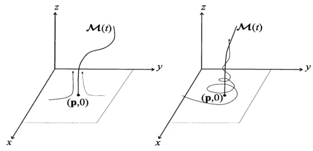
2-1 _{Unsteady separation profiles emanating from separation points (p,O) viewed as} a time-dependent material line that guides particles away from the wall. . . . 27

2-2 M oving boundary. . . . 32

2-3 Reattachment profile as a time-dependent stable manifold for the point of sepa-ration . . . 44

2-4 Behavior of wall-bound material lines near a reattachment profile in backward tim e. . . . 4 5 2-5 Moving separation along a no-slip boundary . . . 46

3-1 Flow emanating from a sink. . . . 53

3-2 _{Predicted and real saddle-sink separation profiles. . . . 57}

3-3 Approximate and real separation for the saddle-saddle type separation . . . 59

3-4 Visualization of the separation in the case of saddle-focus. . . . 60

3-5 Skin friction fied of the separation bubble. . . . 62

3-6 Visualization of the accuracy of the computed profiles with respect to the sep-aration in the steady bubble flow. Left: streamlines passing under the bubble. Right: streamlines passing over the bubble. . . . 69

3-7 Some slides of the visualization of separation on a bubble; we showed the skin friction field, the periodic predicted profiles of separation at second-order, the periodic surfaces of separation and a few trajectories. . . . 71

3-8 Separation on a closing bubble. . . . 74

3-9 Separation on a non-closing bubble. . . . 75

3-11 Separation over the aperiodic non-closing bubble. Even if the flow is aperiodic,

separation is fixed! . . . 81

4-1 Separation surface. . . . 84

A-i The definition of the flower-cone

Q.

. . . .. 94

A-2 Fluid particles entering and leaving the flower-cone

Q.

. . . 95

B-i Predicted and real saddle-focus separation profiles. . . . 105

B-2 Saddle-focus separation profiles at different orders. . . . 108

B-3 Saddle-focus separation profiles at increasing orders. . . . 111

Introduction

Preliminaries

The theory of separation was initiated by Ludwig von Prandtl in 1904 who showed that stream-lines in a steady flow past a two-dimensional streamlined body separate from the boundary where the skin friction vanishes and admits a negative gradient. If we define y = 0 to be the flat boundary of a two-dimensional steady velocity field (u(x, y), v(x, y)), the skin friction -, along the wall must satisfy a set of conditions at a separation point (p, 0):

TW(p) = vp(p, 0) Uy(p, ) = , ₍₁₎

T'W(p) = _{VP(p, 0)U2.y(p, 0) < ,}

where v is the kinematic viscosity and p is the density of the fluid.

For a long time, these conditions have been considered the definition of separation, until Rott (1956), Moore (1958) and Sears & Telionis (1971) proved that zero skin friction does not caracterize separation in unsteady flows. This lead to a change of the definition of separation for unsteady flows and yielded the Moore-Rott-Sears (MRS) principle. This principle, however, requires that we know the separation speed; indeed, Williams (1977) and Van Dommelen (1981) explained why this principle is difficult to apply.

Van Dommelen (1981) and Van Dommelen & Shen (1982) were the first to study unsteady boundary-layer separation in Lagrangian coordinates. The computational simplifications ren-dered by this method revealed that unsteady separation is in essence Lagrangian. Cowley, Van Dommelen & Lam (1990) showed that separation is caracterized by contraction towards a point, accompanied by a spiky expansion in the wall-normal direction at that point. The Lagrangian notion of separation was further studied by Peridier (1995), Cassel, Smith & Walker (1996), Degani, Walker & Smith (1998). Formal asymptotic expansions for Van Dommelen's singularity in the boundary-layer equations have been obtained by Cowley (1983) and Van Dommelen &

Cowley (1990).

Although boundary-layer separation has been numerically studied very accurately, no satis-fying theory has been formulated. Moreover, because separation occurs both for low and high Reynolds numbers, one should be able to study separation without solving the boundary-layer equations. Indeed, Sears & Telionis (1975) pointed out the need for an unsteady separation definition that does not depend on boundary layers. Moreover, Cowley et al. (1990) stressed that an ideal separation definition which would be independent of the coordinate system. Fi-nally, active flow control forced Wu, Tramel, Zhu & Yin (2000) to seek a separation criterion that only uses quantities obtained along the boundary.

The conditions (1) are purely kinematic: They can be derived for any two-dimensional steady vector field that conserves mass, as shown by Shariff, Pulliam & Ottino (1991). Moreover, the Lagrangian definition of steady separation has the above three ingredients, and was the starting point of Shariff et al. (1991): For two-dimensional, incompressible, time-periodic flows, the separation point is a fixed point with an unstable manifold for the Poincar6 map associated with the flow. They showed that unsteady separation takes place where the time-average of the skin friction vanishes. Yuster & Hackborn (1997) re-derived this result in more rigorous terms for near-steady, time-periodic, incompressible flows, and Hackborn, Ulucakli & Yuster (1997) verified it experimentally. The latter authors, however, also showed that the principle of zero-mean-skin-friction fails for compressible time-periodic flows.

Haller (2002) analyzed the steady flow separation as an instability in the Lagrangian frame, which is due to the presence of a distinguished fixed point (the separation point) with an unstable manifold. This manifold acts as an attracting material line that collects and transports particles away from the wall. The distinguished fixed point is degenerate due to the no-slip boundary conditions, and hence its location and stability cannot be predicted from linearization. Prandtl's first condition in (1) gives a necessary condition for the existence of such a degenerate fixed point, while (1) as a whole gives a sufficient set of conditions for the existence of an unstable manifold. Haller then extended the Lagrangian separation definition of Shariff et al. (1991) to compressible two-dimensional velocity fields with general time dependence. Specifically, one can define unsteady flow separation as a material instability due to an unstable manifold emanating from a fixed boundary point. Then unstable manifold is a time-dependent material line that

shrinks to the separation point in backward time. In forward time, the unstable manifold attracts and repels particles from a vicinity of the boundary.

Using the above Lagrangian definition, Haller (2002) derive mathematically exact Eulerian criteria that locate the separation point. Due to nonhyperbolicity of fixed points on a no-slip wall, classical dynamical systems methods for locating their unstable manifolds fail to apply. To overcome these limitations of classical invariant manifold theory, Haller (2002) uses a novel nonlinear technique that gives both the location and the shape of unstable manifolds, that are named separation profiles. This approach only assumes local mass conservation and regularity for the unsteady velocity field.

We show on a practical example the validity of the above theory: The analysis of separation over a pitching airfoil is a matter of interest to the aerodynamics community. We then consider a relevant example of an airfoil: a NACA 0012. We change periodically its angle of attack, and use a Navier-Stokes solver (developed by Hesthaven 1998) to derive the flow around the airfoil. Using Haller's formulae restricted to the upper surface of the airfoil allows us to analyze aperiodic separation.

As fluid flows are rarely two-dimensional, the matter of three-dimensional separation has received a lot of interest for decades. Different definitions of separation have been proposed, some highly contentious.

Legendre (1956) and Lighthill (1963) were the first to introduce a theoretical treatment of three-dimensional separation. Without proposing a theory that would predict 3D steady separation, they describe separation with geometrical arguments. The topological classification of Chapman (1986) distinguishes a great number of separation shapes, contrary to the relative simplicity of two-dimensional separation geometry. Here we show in figure 0-1 three basic shapes of separation: saddle-sink, saddle-saddle and saddle-focus.

Streamtines/

Saddle-sink Saddle-saddle Saddedcu

separation '"' separation separation

point point point

Figure 0-1: Three basic shapes of separation: saddle-sink, saddle-saddle and saddle-focus.

Further work by Wang (1970) introduced the concept of open separation: contrary to the two-dimensional case, one can observe separation (along a surface) while there is no observed specific separation point. First highly criticized, this concept has been adopted by others (see Wang 1983 for details). One can now define steady separation as a breakaway of particles from the wall. Closed separation occurs at a zero skin friction point, which acts as a distinguished separation point (and may also be part of a separation surface). By contrast, open separation does not occur at a zero skin friction point: there is no distinguished separation point but a separation surface, whose intersection with the wall (the separation line) is a skin friction line. A similar definition for any unsteady flow has, however, always been missing. Here we define closed separation as a case of separation (particles breaking away from the wall) where there is at least one distinguished separation point; we call the separation open when there is no such point. When the flow is steady, the two definitions coincide.

Later work has concentrated on the experimental verifications of the geometrical concepts of three-dimensional separation, which are of vital importance in a wide range of engineering ap-plications. For instance, separation drives the formation of vortices over a surface, as explained by Wu & Gu (1987). One can also study the transition to turbulence and fully developed turbulence of various wall-bounded flows. A lot of related numerical computations have been performed by Legendre and Werl6 (D61ery 2001).

With the increasing development of computational fluid dynamics, one needs a quantitative criterion to characterize separation. As for now, only a topological theory has been introduced: the critical point theory of Perry & Chong (1987), which classifies steady separation points in geometrical terms; an analysis of the topology of pressure surfaces (Tobak and Coon 1996) which links separation surfaces to pressure surfaces; and a vorticity dynamics theory (Wu et al. 2000) which analyzes the on-wall signatures of separation, and shows that closed separation occurs at zero skin friction points. These theories generally describe the flow in an Eulerian way, and only focus on steady incompressible flows. The ideas they introduce are qualitative and geometric, and only apply to steady flows. So far, an understanding of three-dimensional unsteady separation has been missing, and no theory has ever been presented.

In his previous work on two-dimensional separation, Haller (2002) analyzed unsteady 2D separation; his theory is here extended to three-dimensional unsteady separation. The main

result is that fixed closed separation takes place where the weighted backward-time average of the skin friction remains uniformly bounded. The weight function in the average is just the squared reciprocal of the fluid density. We also introduce the concept of effective separation points at which the finite-time mean of the skin friction vanishes. Numerically, these points converge to the fixed separation points.

To validate this new theory, we derive some three-dimensional separated flow models using a concept developed by Perry & Chong (1986). We present the three basic shapes caracterizing steady closed separation: saddle-sink, saddle-saddle and saddle-focus separation, showing how the predicted separation profile fits the observed shape of separation. Then we develop a new model: a separation bubble, with an interesting pattern of separation. We study different kinds of unsteadiness on this model: periodic and quasiperiodic.

Finally, we explain the current limits of our theory and propose further extensions.

Thesis outline

The outline of this thesis is as follows.

In chapter 1, we review the kinematic theory of 2D unsteady separation from Haller (2002) and apply it to a relevant example. The first part of this chapter is mostly intended to recall the concepts of separation, separation point and separation profile. The second part of chapter 1 focuses on the validation of the theory in the unsteady case: we analyze the flow around a two-dimensional pitching airfoil, and show how, under certain conditions, separation happens on the upper part of this airfoil. We shall also develop some concepts for the control of separation. In chapter 2, we extend Haller's theory of separation to three-dimensional flows. We define closed and open separation, then concentrate on closed separation. We still use the concepts of separation point, separation profile or moving separation.

In chapter 3, we use a method developed by Perry & Chong (1986) to introduce physically relevant incompressible expansions of the Navier-Stokes equations to be used as models of three-dimensional separation. These flow models allow us to verify our separation theory on relevant steady, periodic and quasiperiodic examples. We first introduce a steady model that contains the three separation patterns one typically observes: saddle-sink, saddle-saddle and saddle focus. Secondly, we present a three-dimensional model of a separation bubble flow, both for the steady and the unsteady cases. On this model, we illustrate the usual concepts of three-dimensional unsteady separation points and profiles. In addition, we also explain the genuinely three-dimensional concepts of separation lines and separation surfaces.

In chapter 4, we focus on a new approach to separation lines and surfaces. We discuss initial results for these objects, and outline the next steps to be taken in their study.

Finally, we present our conclusions.

In appendix A, we derive the proofs and formulae used in our three-dimensional separation theory.

In appendix B, we present details of the arguments used in the validation of the three-dimensional theory.

Chapter 1

Location and shape of aperiodic

separation over a pitching airfoil

1.1

Introduction

The objective of this chapter is to visualize the points and angles of separation in an unsteady flow over a pitching airfoil. This method can be applied to a wide range of vehicles, such as passenger cars, submarines, etc.

The pitching airfoil is investigated as an example to detect and control dynamic stall. Prob-lems involving unsteady separation over aerodynamic boundary layers are usually modeled as nominally two-dimensional flows over a moving airfoil. As explained by Sinha et al. (1997), such models contain the essential characteristics of dynamic stall on helicopter rotors, where stall occurs during the pitch-up motion of the blade of a rotor. Particles can separate from the upper part of the airfoil, which causes fatigue failure in the blade control mechanisms, as well as loss of lift.

The above problem has been studied experimentally by Pal et al. (1997) and numerically by Okong'o & Knight (1997), but a full understanding of stall has not been achieved. More recently, Kuo & Hsieh (2001) analyzed the structure of separation over a pitching airfoil using vortex visualization. New simulations and experiments by Magil et al. (2001), Reuster & Baeder (2001) and Emblemsvag et al. (2002) aim to control separation over pitching airfoils. Here we shall use Haller's (2002) criteria for separation to analyze separation over a pitching airfoil.

The organization of this chapter is as follows. We first recall the main points of Haller's theory in

§

1.2. Then we present an airfoil model, and study separation over it in

§

1.3. We finally present our conclusions in

§

1.4.

1.2

Brief Review of Separation Criteria

1.2.1 Introduction

For convenience, we briefly recall criteria developed by Haller (2002) for unsteady separation points and angles. Consider a two-dimensional velocity field v(x, y, t) = (u(x, y, t),

v(x,

y,

t)),

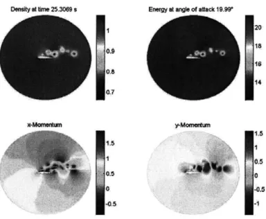
DensIty at Ime 25.3069 s Energy at angle of stack 19.W

4 20

14

X-MoaWn y-Mornedum

Figure 1-1: Flow over a pitching airfoil.

with the induced fluid particle motion satisfying

=u(x, y, t), y=v(x, y, t).

Assume further that a boundary is present in the flow at y = 0 with the no-slip boundary conditions

u(x, 0, t) = v(x, 0, t) = 0.

We also assume that no sinks or sources are present at separation, and hence the continuity equation

Pt + V - (pv) = 0 (1.1)

holds for the density p(x, y, t) in a neighborhood of a separation point (x, y) = (y, 0) .

We seek a time-dependent material line M(t)-the separation profile-that collects and ejects fluid particles from a vicinity of the boundary. As a material line, M(t) is anchored to a boundary point -y due to the no-slip boundary conditions. In dynamical systems terms, M(t) is an unstable manifold for a fixed point of the y = 0 boundary.

Suppose the separation profile is represented by a time-dependent graph x = y + yF(y, t),

F(y, t) has a series expansion

F(y, t) = fo(t) + yfi(t) +

-where

fo(t) = F(O,t), fi(t) = Fy (0, t). Thus, the angle

<p

of separation at time to with the x-axis is

1

= _arctan fo(to)

The explicit criteria and formulae for the point and profile of separation are as follow. 1.2.2 Non-flat boundary

Assuming now that the velocity field satisfies no-slip boundary conditions along a boundary B, we want to find a necessary condition for separation at a point whose relative location is fixed on the non-flat boundary. If the boundary is represented by a differentiable graph y = h(x), as indicated in figure 1-2, we transform the velocity field to a canonical form by letting

(1.2)

Y

y=Jh(x)

OM x

Figure 1-2: Separation over a non-flat boundary.

Compressibility or incompressibility is unaffected by the change of coordinates (x, y)

-(),

j). We only need to apply the previous change of variables in all separation formulae given below.

1.2.3 Necessary Condition

The necessary condition for the separation point

y(to)

at time to is

0

d

to-T 'dT _to d p(y(to), _{0, s) /O} dx p(-y(to), 0, s) T=O >0. (1.3) = x, 71 = y - h( ). d ( JO o- _{Y (_Y(to), 0, s) d,} dT o p(-Y(to), 0, s) T=O

These two conditions represent an extension of Prandtl's necessary criteria to moving separation. Here (g) (x, to, -) is a low-order polynomial least-square fit to sampled values of g(X, to, -) over a T interval as large as possible. This practically means a least-square polynomial fit for g values up to T =

to

-too, where too is the earliest time at which velocity data is available. For a faithful approximation of (g), the order of the least-square polynomial should be low relative to the number of sampled values for g. The slope fo(to) of the separation profile at t = to is given by

p(to)$ /to-T Fb) a) a)(r) - a r

P 2L)a~T

Lto

f, 2S- ds + bx(i-)

f

acs) ds) dT~

fo(to)

-

d(r)

T=O (1.4)

fito-

ax~r -by1 2bx(T)r Vs) ds d, where a(t) = uy(-,0,t), ax(t) = UXY (-, 0, t), 1 ay(t) = (70) b(t) = vy(-,0,t), bx(t) = vxy (7, 0, t), by (t) = Y b (7, 0, 0), 1 p(t) = pb, 0, ) 1.2.4 Sufficient Condition

First, for the present time to, we compute the effective separation point 'Yeff(t, to) for all available t < to, which is obtained via the formula

ft

Uy( eff , 0, T) dT = 0. (1.5)

i PCbeffA-) We then identify the upper and lower bounds

(t o) = sup 7eff (s, to), y-(t, to) = inf Yeff (s, to),

sE[t,to) sE[t,to)

on 'Yeff(t, to). Let the maximal x distance travelled by -yeff(s, to) over the interval [t, to) be denoted by

6(t, to) = Y+(t, to) - Y_ (t, to), which is the length of the interval

One can then prove the existence of finite-time separation at the point

'"y(to) =

[}+

(to - Tm(to), to) + _Y (to - Tm(to), to)] , (1.6) where T,(to) is the smallest time for which

1 ito

-J(t, to) max IuxY(x, 0, t)I dt = 1, (1.7)

2 -Tm(to) xEI(to -Tm (to),to)

max uxy(x,0, t) < 0, t E [to - Tm(to), to] x EI(to-T,, (to),to)

The above conditions distinguish one finite-time unstable manifold out of the infinitely many near the moving separation point.

The moving separation slope is given by the formula

p(to) ₀ )b(r) a(t) ds + b(T) r s) ds - a(T d

fA(to) - 2b. - (1.8)

ftoT.(to) a r) bxr P(3- s

1.3

Separation over a pitching airfoil

1.3.1 Model

The first part of this work consists of defining the airfoil to be studied. We consider the most common airfoil, the NACA 0012. In such an airfoil of the National Advisory Committee for Aeronautics with four digits, say MPXX, the digit M represents the maximum value of the mean line in hundredths of the chord, P represents the chordwise position of the maximum camber in tenths of the chord, and the number XX is the maximum thickness in percent of the chord.

The equation of the upper boundary of this airfoil is given by

y = 1(x) = 0.17735V/ - 0.075597x - 0.212836x2 + 0.17363X3 - 0.06254x4.

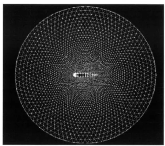
The lower boundary is symmetric. We translate this airfoil to place it in the middle of our numerical grid. The length of the airfoil is one; it is placed in the center of a circle of radius 3, as shown in figure 1-3.

1.3.2 Aperiodic flow

When the inflow is steady, the flow developing near the airfoil is periodic or quasiperiodic, with vortices behind the airfoil. When the inflow is periodic, the developing flow tends to be aperiodic. In the latter case, we periodically (period = 10s) change the angle of attack of the airfoil between -5 to +15 degrees. Under such flow conditions, the airfoil is said to be pitching.

Figure 1-3: Mesh of the pitching airfoil.

1.3.3 Separation

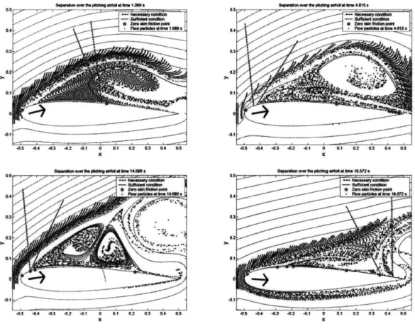
We use a Navier-Stokes solver developed by Hesthaven (1998) to generate the velocity field around the airfoil. We then use the method explained in § 1.2 to find the zero skin friction points, and evaluate the sufficient and necessary separation points. Figure 1-6 underlines the difference between the zero skin friction points and the separation points.

Computation

We use both the necessary and the sufficient criteria in Section 1.2 to determine the approximate points and angles of separation. For the necessary condition, we use a third-order polynomial least-square fit to extract the mean components. Figure 1-4 shows that such a fit well captures the profiles of sampled values of fto Y(to)O ds and

ato-T

by(rax(r) _{to p~) io ps)ds} Usr ds + b.(r) _b~T) \Jt ps) a)dsr /s -p - (,r)

1

dr, respectively.

For the sufficient condition, the time scale T is determined by (1.7) and is shown in figure 1-5.

Visualization of separation

We compute the approximate points and angles of separation through formulae (1.4) and (2.5), as shown in figure 1-6. We track the particles and show the zero skin friction points, and the necessary and sufficient separation points along with their slopes (see the legend of the figure for explanation). We conclude that our formulae give a good approximation of the separation point and angle. Indeed, the two separating lines are close to the exact separation profile along which the spikes of fluid particles are formed. Furthermore, we see that the zero skin friction point is not the point of separation; this disproves the common belief that the zero skin friction point is the point of separation in unsteady flows.

I

Figure 1-4: Third-order polynomial least-square fit to sampled values of fto to),Os) d('y and fo"-T

[by(r) (T) ds + ba(r)

(

f ds dr, respectively.

Figure lation.

1-5: Time-scale determined by (1.7) for the sufficient condition in the separation

simu-1.3.4 Control of separation

A next step of this analysis will be, instead of looking at separation, trying to control it. We still need an efficient device capable of controlling the phenomenon of separation, which creates losses of drag and lift.

Wang et al. (2003) established a feedback control law to control separation in two-dimensional shear flows. Work by Salman et al. (2002) established a feedback control law for Stokes flows, noting that the same control law fails for Navier-Stokes flows. This failure is due to inertia-related delays in real flows, as explained by Insperger (2003). Later work has concentrated on implementing delays in the controller; preliminary results by Lekien et al. (2003) are promising.

1.4

Conclusion

We have performed numerical simulations for real-time monitoring of separation points and angles in the unsteady pitching of an airfoil. These simulations showed Haller's criteria for

- df -OW' a 4 6 a G t 2 0 to 20 30 40 W

1:-. CWft

I

I

---

---

----0 ID 20 30 40 t

A$ 4 413 02 01 6001 02 S CA - 0442 41 9 01b W0 0w, XX 02-01 -03 49A 43 4,2 -0,1 0 0*1 02 0.3 0.4 A5 414 04 2 -0 02 41 0 401 0'2 03 0A4 02 x x

Figure 1-6: Separation over the pitching airfoil.

separation in two-dimensional unsteady flow to be accurate. We have also found that the zero skin friction point is not the point of separation, and that the behavior of the separation point depends on the flow. If the flow is periodic, or quasiperiodic, the separation point is fixed; If the flow is aperiodic, the separation point appears to move, but its motion is unrelated to that of the zero skin friction point.

Chapter 2

Kinematic theory of

three-dimensional unsteady flow

separation

2.1

Introduction

In his work on two-dimensional separation, Haller (2002) analyzed unsteady 2D separation as a material instability due to an unstable manifold emanating from a fixed boundary point and extended Prandtl's formulae to any unsteady flow: He derived mathematically exact Eulerian criteria that locate the separation point and obtained both the location and the shape of the unstable manifolds that generate the separation profiles.

As explained in the introduction, Wang (1970) introduced the concept of open separation: contrary to the two-dimensional case, one can observe separation (along a surface) while there is no observed specific separation point. We define closed separation as a case of separation (particles breaking away from the wall) where there is at least one distinguished separation point; we call the separation open when there is no such point. When the flow is steady, our definition coincide with Wang's.

Haller's theory is here extended to three-dimensional unsteady separation. The main result is that fixed closed separation takes place where the weighted backward-time average of the skin friction remains uniformly bounded. The weight function in the average is just the squared reciprocal of the fluid density.

The organization of this chapter is as follows. We first derive necessary conditions for fixed compressible separation in

§

2.2, where we also give a first-order approximation for a general compressible separation profile. Section 2.2 also contains equivalent Lagrangian and density-independent formulations of our criteria, as well as a version for moving boundaries. We show how the theory simplifies for incompressible flows in

§

2.3, and exploit this simplification to derive a third order approximation for incompressible separation profiles. In

§

2.4 we give a kinetic version of the separation criteria for Navier-Stokes flows, and in

§

2.5 we formulate sufficient conditions for sharp unsteady separation. Section 2.6 explores how our fixed separation criteria simplify to steady, time-periodic and quasiperiodic flows. Unsteady reattachment is discussed in

§

2.7, and we deal with the difficult problem of moving separation in

§

2.8. We will

finally present our conclusions and some open problems in

@

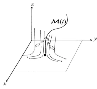
2.9.

2.2

Fixed unsteady separation

2.2.1 Set-up

Let us consider a three-dimensional unsteady velocity field

v(x, y, z, t) = (u(x, y, z, t), v(x, y, z, t), w(x, y, z, t)) which admits a boundary at z = 0, with

u(x, y, 0, t) = v(x, y, 0, t) = w(x, y, 0, t) = 0. (2.1) To distinguish the velocity components parallel to the boundary, we shall use the shorthand notation x = (x, y) and

u(x, z, t) = (u(x, y, z, t), v(x, y, z, t)) , w(x, z, t) = w(x, y, z, t).

Fluid particle motions satisfy the three-dimensional system of differential equations of mo-tion

0=

u(x, y, z, t), i = v(x, y, z, t), i = w(x, y, z, t), (2.2) or, briefly,

x = u(x,z,t), = w(x, z, t),

We seek a time-dependent material line M(t)-the separation profile-that collects and ejects fluid particles from a vicinity of the boundary. We also seek a surface of separation which attracts all particles away from the wall. The separation profile is a material curve that attracts all fluid particles within the separation surface. The separation surface may be degenerate: It may just coincide with M(t). An example of this type of separation is given by tornado-type vortex formation near the boundary.

To exclude degenerate or unphysical cases of separation, we shall only consider separation profiles with the following properties:

1. The separation profile is unique: no other separation profiles emerges from the same boundary point.

2. The separation profile is transverse, i.e., M(t) is not tangent to the boundary.

3. The separation profile is regular up to nth order: M(t) admits n derivatives (n > 1) that remain uniformly bounded at y = 0 for all times.

2.2.2 Assumptions

Assuming that no sinks or sources are present at separation, the continuity equation

z

MW(t)

(pO)

x z x

Figure 2-1: Unsteady separation profiles emanating from separation points time-dependent material line that guides particles away from the wall. is satisfied in a neighborhood of a separation point (x, z) = (y, 0). The conditions at z = 0 simplifies the continuity equation to

pt (x, 0, t) + p(x, 0, t)wz(x, 0, t) = 0 at boundary points and implies

(p,O) viewed as a

no-slip boundary

p(x, 0, t) = p(x, 0, to)e-

fi

w(x,0,s) ds _(2.4)

Differentiation of (2.4) with respect to x and y gives the wall-tangential density gradient evo-lution

pX(x, 0, t) = px(x, 0, to)e-

ft

wz(x,0,s) ds -p(x, 0, to)e ,f w (x,O,s) ds wt 2(x, 0, s) ds. (2.5) Here and in later formulae, the subscript x refers to the gradient operation with respect to the variables x and y.

As the density of the fluid should remain bounded from below and from above for all times along the boundary, for appropriate P2 > Pi > 0 and for all t,

0 < Pi < p(x, 0,t) P2 < 00 _(2.6) must hold along the boundary region of interest.

We also assume that the tangential density gradient along the boundary remains uniformly

M4(t)

bounded near the separation point for all times:

WXZ(X, 0, s) ds < K, < o, (2.7)

for an appropriate constant K1, for any time t, and for all x values near Y.

Assumptions (2.6)-(2.7) hold automatically for incompressible flows, because for such flows, wZ(x,

0,t)

0, wxz(x,0, t) 0.

2.2.3 Equation for the separation profile

We rewrite the velocity field in a form more suitable for separation studies. The no-slip boundary condition simplifies the velocity filed (2.2) to

x = zA(x, zt, = zB(x, z, t), (2.8)

where we define the quantities

1 1

A(x, y, z, t) = , uz(x, s z, t) ds, B(x, z, t) =

Jw(x,

s z, t) ds. (2.9) Fixed unsteady separation occurs if a boundary point p = (-y, 0) admits an unstable manifold M (t) not tangent to the boundary: then we locally represent this manifold

x = Y + zG(z, t).

Changing to the new horizontal coordinates

(

x - -y, we seek the following representation for the separation profile:

= zG(z, t). (2.10)

Substitution of (2.10) into (2.8) yields

z [(B(y + zG, z, t)G + zGz) + Gt - A(y + zG, z,

t

= 0. (2.11) As the separation profile is continuously differentiable, the bracketed expression in (2.11) must vanish for all z > 0. (It is zero for z > 0, and continuity implies that it also vanishes at z = 0.) Then (2.12) implies that the separation profile must satisfy the partial differential equation

Gt = A(-y + zG, z, t) - B(y + yG, z, t) (G + zGz) . (2.12) We call this equation the separation equation; we use it to deduce necessary criteria for separation, then for devising approximations to the separation profile at any order. These approximations are obtained from a series expansion

where

go(t) = G(0, t), gi(t) = Gz(0, t), g2(t) = GZZ(0, t).

2.2.4 Necessary conditions for separation We first simplify our notation and set

a(t) = A(y, 0, t), b(t) = B(y, 0, t), p(t) = p(-y, 0, t),

where (-y, 0) indicates the separation point we wish to characterize. Then the density satisfies

p(t) = p(to)e Jt b(s)ds. (2.14)

When we set z = 0 in the separation equation (2.12), we obtain the linear differential equation

9o(t) = -b(t)go(t) + a(t), (2.15)

whose general solution can be written

go(t) = go(to) + p(t) a(s) ds, (2.16)

p(to) Ito p(s)

using (2.14).

Recall that (go(t))i is the tangent of the angle that the separation profile encloses with the wall-normal direction at = 0, z = 0, in the x-direction, (go(t))2 is the tangent of the angle in the y-direction. Fixed separation takes place at x = -y, if go(t) remains bounded in backward time. By assumption (2.6), the first term on the right-hand side of (2.16) and the p(t) factor in the second term are both bounded in backward time. Therefore, a necessary condition for separation is the boundedness of the integral of the second term in (2.16). Using the skin friction field

r (x, t) = vp(x, 0, t)uz(x, 0, t), (2.17)

we express this boundedness requirement

ft(TQ,0,s)

lim sup

]

Y 0s) ds < oo, _(2.18)

t--oCo to P 2(-y, 0, S)

or, equivalently,

lim sup uz(, 0, S) ds < oc. (2.19)

t--oo Jto p(7Y,0, s)

Just as Prandtl's first two-dimensional separation condition, (2.18) is also satisfied at any point of a fluid at rest, which shows the need for a second condition to describe separation. A second necessary condition turns out to be

[-t ax(s) - bz(s)I _ a(r) 0 bx(s) + bx(s) - a(r)I

lim p)

1pr)dr]

ds = oc, (2.20)

a -snxer to Pth) pde) mttO [

(a)2 (bx)j. Condition (2.20) ensures that all material lines emanating from boundary points

near -y converge to the wall in backward time, a feature that flows at rest do not admit. 2.2.5 Effective separation points

The theoretical necessary condition (2.18) is not suitable for computation. To derive an equiv-alent condition, we again recall that material lines emanating from any boundary point near (y, 0) align with the boundary as t -- -oo. By formula (2.16), this asymptotic alignment in backward time is only possible if, for all small enough Ix - -Yj with x different from y,

lim sup u(x0) ds = +oo.

t-u-oo

ito p(x,O,s)

Defining the integral

it (x) = u(x S) ds J'0 p(x,0,s8)'

we see in the same way as in the two-dimensional case, that it(x) must admit at least one zero that approaches -y as t approaches -oo. As a result, defining the effective separation point 7eff (t, to) via the formula

f UZ(eY',os) ds jt = 0 (2.21)

to P(Yeff ,,s) we obtain

y= lim Yef f(t, to). (2.22)

t-+-oo

We do not prove the existence of the effective separation point (2.21) here; we simply postulate it and find that it works perfectly well in rigorous computations. Equations (2.21) and (2.22) give a practical algorithm for computing fixed unsteady separation points at time to from velocity data. For a past time t with It - to I large enough, one computes the integral in it(x) in the whole plane and finds one effective separation point

gIeff(t, to). By (2.22), this

effective separation point will converge to the real separation point -y as t -+ -00.

Two remarks are in order. First, it turns out that fixed separation points of time-periodic or time-quasiperiodic flows are exactly computable from finite-time velocity data without the use of effective separation points (cf.

§

2.6). Second, taking the limit t -+ -oo in our formulae does not require solving for the velocity field in backward time: It requires computing longer and longer backward-time averages from the available velocity data as the current time to progresses. 2.2.6 Direction of separation

To obtain an expression for the direction of fixed unsteady separation, we first differentiate (2.12) with respect to z and set z = 0 to obtain the differential equation

gi = az + (a. - bI) go - (bx - go) go - 2bgi. (2.23) Our notation here is consistent with that of the previous sections; for instance, we have ax(t) =

Using the density formula (2.14), we write the solution of the above linear ODE in the form gi(t) = gl(to)I2(7) +

.1:

p2(t) [az(s) + (ax(s) - bz(s)I) go(s) - (bx(s) - go(s)) go(s)] ds,

(2.24) where I denotes the 2 x 2 identity matrix. For a second-order separation profile (i.e., for a profile of bounded curvature), the above solution must be bounded as t - -oc. As we show in appendix A.1, this boundedness requirement leads to the following formula for the slope of the separation profile at t = to:

go(to) =--

[

t Q(s, to, t) dsl p(s, to) ds, (2.25)

t+- to _{_ to}

where we define

az(s) ax(s) - bz(s)I S a(r) ( s a(r) 2

p(s, to) = p()+ p~)

]~dr

- by (s)

y'~

dr)

p 2(S) p(S) to plr) to PCTr)

Q

(S to, t) - I [ax(s) - bz(s)I /.s a(r) 9 bx(s) + bx(s) - a(r)I dr (2.26)

p(to) p(s) to p(r) (

Similar expressions can be derived for higher-order derivatives of G(z, t) in a recursive fashion by further differentiating the separation equation (2.12) with respect to z at z = 0.

2.2.7 Density-independent formulation

Using the density relation (2.4), we can express the density in terms of the integral of wz (y, 0, t), and obtain a density-independent formulation of our separation theory. In this formulation, assumptions (2.6) and (2.7) are expressed as

wz(x, 0, s) ds < Ko < oo, wxz(x, 0, r) dr Ki < oo,

.1to _t

and the separation criteria (2.18) and (2.20) are replaced by

lim sup e O ,0 ) dsz' 0, T) dw < oo (2.27)

t--+-oo

Jto

and

~lo

im

ef; wz(yOs)ds _(ad(s) - Ibz(s))

(ef

w(7,,s) ds(a(r) 0 bx(s) + bx(s) - a(r)I) dr) ds = o. (2.28)

Similarly, effective separation points are defined by the formula

The separation slope and curvature, as well as higher order derivatives of the separation profile can all be expressed in purely kinematic terms using the density relation (2.4). We shall use the above density-independent formulation in deriving separation conditions for moving boundaries in

§

2.2.8.

2.2.8 Separation on moving boundaries of general shape

Let us assume now that the velocity field (2.8) satisfies no-slip boundary conditions along a boundary B(t) which is not flat and steady but moves with velocity vB(t) = (US(t), wB(t)). Thus we would like to find a necessary condition for separation at a point whose relative location

is fixed on the moving boundary. As the previous formulae are not directly applicable, we need to transform them.

If at time to the boundary-say, a moving airfoil-is represented by a differentiable graph z = h(x), then at a later time t the boundary satisfies

z -

j

wB(s) ds = h(x -

j

un(s) ds),

to t 0

as indicated in figure 2-2.

z

x

Figure 2-2: Moving boundary.

Then we transform the velocity field to the canonical form (2.2) by setting

= x - u (s) ds, 7 = z - h() - fwS(s) ds. (2.30)

In terms of the

((,

r) coordinates, fluid particle motions satisfy = 'C( , 77, t), I = fs( , 77, t),

with the new velocity field

((, t) = u( +

I:

U3(s) ds, r + h

()

+

/

w8(s) ds, t) - uB (t),

t((, r/, t) = w( +

ft

U3(s) ds, 97 + h( ) +

Jt

wB(s) ds, t) - wB3(t) - h'(,) - i(, 7, t).

t0t

The transformed velocity field (fi, zb) satisfies the boundary conditions

fi(x, 0, t) = 0, '(x, 0, t) 0. (2.31)

Furthermore,

Tr fl + zi Trux + h' -u, + whf -uz = Tr ux + wz,

which corresponds to the continuity equation (2.36), thus compressibility or incompressibility is unaffected by the change of coordinates (x, z) -4 (, rI) .

Because

(, 0, t) = uz(( + j us(s) ds, 9 + h( ) + jwB(s) ds, t), (2.32)

t t

7(, r7, t) = wz( +-f uB(s) ds, 9 + h( ) + jw (s) ds, t) - h'() - fiq r7, t),

t t

the density-independent necessary condition (2.27)-applied in the ( , rI) coordinates-takes the form

lim sup fE(-y, T, t) uz(-y + u(s) ds, h(-y) + w1(r) dr, ) dT <00, (2.33) where

E(-, r, t) exp wz ( + u3(r) dr, h(-y) + w1(r) dr, s)

to - t'O J10

-h'(y) -uz(-y +

f

u3(r) dr, h(y) +

/

wi(r) dr, s)] ds. (2.34) As in the case of flat boundaries, we locate the separation point on general boundaries by computing the effective separation point yeff(t, to) for

It

-

toI

large enough from the formula

ft

E(yejf, r, t) uz(-y +

f

u3(s) ds, h(-yeff) +

j'

wB(r) dr, T) dT = 0. (2.35)

To evaluate the second necessary condition (2.28) in the present ( , 97) coordinates, we compute the second derivatives

i tfi rom (3, Wit th se( er h, s

condition (2.28) becomes a straightforward but lengthy condition, which we omit here for brevity.

2.3

Fixed unsteady separation in incompressible flows

In this section, we consider incompressible flows, and show how our theory for fixed unsteady separation simplifies in this case. (We also derive a general third-order approximation for the separation profile.)

2.3.1 Set-up

Consider again the velocity field (2.2), but which also satisfies the incompressibility condition

Tr ux + wz = 0. (2.36)

The no-slip boundary conditions again enable us to rewrite the velocity field in the form (2.8), with the equivalent incompressibility condition

zTrAx + B + zB, = 0.

Setting z = 0 in this equation gives B(x, 0, t) 0, thus we can further rewrite the velocity field in the form

x = zA(x, zt, = z2C(x, z, t), (2.37)

where we have

C(x, z, t) = wzz(x, spz, t)p dp ds. (2.38)

Enforcing the incompressibility condition (2.36) for system (2.37) yields

z (Tr Ax + 2C + zCz) = 0. (2.39)

Away from the boundary, i.e., for z > 0, this relation between the functions A and C implies

TrAx + 2C + zCz = 0. (2.40)

Because Ax, C, and Cz are continuous, this last equation extends to z = 0. Therefore, (2.40) must hold all over the fluid, including the boundary.

In our arguments, we will work with the incompressible canonical velocity field (2.37) for simplicity. Alternatively, one could work with the compressible canonical form (2.8) and use the incompressibility condition (2.40), but that approach would quickly lead to intractably complex expressions.

2.3.2 Equation for the separation profile

As in the compressible case, we want to express the unsteady separation profile as an unstable manifold satisfying = x - - = zG(z, t). Differentiating in time and substituting this relation

into (2.37) implies

z [A(zG + -y, z, t) -- zC(zG + -y, z, t) (G + zGz) - Gt] = 0. By continuity, the bracketed expression must vanish for all z > 0, which yields

A(zG + y, z, t) - zC(zG + -y, z, t) (G + zG,) - Gt = 0. (2.41) Applying the incompressibility relation to the compressible separation equation (2.12), we also recover (2.41).

2.3.3 Necessary conditions for separation

We now write the constant term in the Taylor expansion of the incompressible relation (2.41) and obtain the differential equation

go = a. We integrate this equation to obtain

go(t) = go(to) +

j

a(T) dT. (2.42)

As at the point (y, 0) we require go(t) to be bounded in backward time, we obtain the first necessary condition:

limsup uZ(y, 0,T) dT < 00. (2.43)

t--oo

Re-applying the ideas in (2.20) and the proof of appendix A.1, we obtain the second necessary condition at fixed separation points:

lim

f

(a(-y, 0, r) + I Tr a(-y, 0,,T)/2)dT = 00. (2.44)

2.3.4 Effective separation points

As the separation criterion (2.43) is unsuitable for direct computations, we still use the effective separation point principle. Effective separation points are now defined as

/

Uz(ef f (to, t), 0, s) ds = 0. (2.45)

They approximate the location of the actual flow separation. Our argument for the convergence of effective separation points to actual separation points applies here again.

2.3.5 Separation profile up to third order

We now give explicit formulae for the time-dependent coefficients of the cubic separation profile