a. Additional information about the EICAT assessment procedure

(1)

a. Additional information about the EICAT assessment procedure

Uncertainty rationales

Confidence levels (high, medium or low) are assigned to each observation to indicate how confident the assessor is that the assigned magnitude is the ‘true’ one: the assessor therefore evaluates the chances that the ‘true’ impact magnitude is different from the one assigned (IUCN, 2020b; Volery et al., 2020). A High confidence level is assigned to an impact observation only when the assessor is confident that the assigned magnitude is the true one, i.e. that higher or lower impact magnitudes are unlikely according to the impact description and methodology of the study. A Medium confidence level is assigned when evidence indicates that the true impact magnitude is likely to be the one assigned, but that be a higher or lower magnitude is also possible. When the assessor did not find evidence indicating that the true impact magnitude is likely to be the assigned one, a Low confidence level was assigned. A Low confidence level can be assigned to vague impact observations with few or no details on the experimental or observational set-up, but also to well-designed studies testing effects not easily transferrable into EICAT criteria.

In our study, to increase transparency on how the confidence levels were assigned and to highlight where uncertainty occurs in each observation, the assessor evaluated if the true impact could be higher or lower than the one described, based on the described impact in the report and considering the methodology for observing it (see Sheet 4 in Supp. 2).

For example, if a field study finds decreases in performance of individuals of a native species (observed impact = MN), but did not look at changes in its population density, it is possible that the true impact might even have led to a population decrease (MO) (IUCN, 2020b; Probert et al., 2020; Volery et al., 2020). It is however unlikely that the impact is negligible (MC) as the decrease in the performance of native individuals was observed; it is also unlikely that the alien led to a local extinction (MR/MV) as individuals were observed. This approach led to higher consistency among the three assessors.

Species guilds

Deer are often forming guilds of several species, making it difficult to evaluate the impact of a species independently

from the others (e.g. Wardle, Barker, Yeates, Bonner, & Ghani, 2001). When the experimental set-up did not allow

distinguishing the individual impacts of each species, we assigned the described impact to all alien species in the guild

and decreased the confidence level. For instance, if a species was the most abundant in the guild, it is likely that this

species was contributing to the described impacts (no decrease in the confidence level), whereas if a species comprised

only a small part of the guild, it is less clear whether it contributed to the described impact or whether the same impact

would have been occurring in its absence (decrease in confidence level).

(2)

Complementary studies

In a few cases where multiple studies where explicitly complementing each other, the assessor combined them into one

impact observation (see Sheet 4 in Supp. 2). For instance, one study was observing the change in the native population

(e.g. a decline in the population size), and another study was establishing the link between this change and the alien

(e.g. by showing the mechanism through which the alien is acting on the native population). This was to avoid double

counting of impacts. When the link between two studies was not explicitly made in the reports, we did not combine

studies.

(3)

b. R code for the significance test of pairwise comparisons between impact risks To compare the impact risk of Species

a

with the impact risk of Species

b

:

# Generating beta distributions for Species

a

and Species

b

, based on the frequency at which they caused their highest impact a <- rbeta(number_of_simulations, (Species

a

_number_of_successes + 1), (Species

a

_number_of_failures + 1)) (where “successes”

indicate the number of regions in which Species

a

caused its highest impact magnitudes, and “failures” indicate the number of regions in which it caused lower impacts)

b <- rbeta(number_of_simulations, (Species

b

_number_of_successes + 1), (Species

b

_number_of_failures + 1))

# Comparing the two distributions by calculating their overlap sum((a-b)>0)/number_of_simulations

sum((b-a)>0)/number_of_simulations

We used 100’000 simulations to generate random beta distributions. The lowest overlap measure is taken as the p-

value: values around 0.5 indicate a complete overlap of the two probability distributions, whereas values around 0

indicate almost no overlap and allow to reject the null hypothesis that the two probability distributions are not different.

(4)

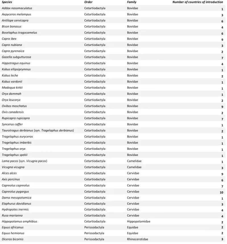
Table S1. Species classified as Data Deficient (DD). To test whether more widely ungulates were more often studied (see Table S8), we added the numbers of countries each species has been introduced to (no re-introductions) (extracted from Sheet 3 in Supp. 2).

Species Order Family Number of countries of introduction

Addax nasomaculatus Cetartiodactyla Bovidae 1

Aepyceros melampus Cetartiodactyla Bovidae 3

Antilope cervicapra Cetartiodactyla Bovidae 6

Bison bonasus Cetartiodactyla Bovidae 4

Boselaphus tragocamelus Cetartiodactyla Bovidae 6

Capra ibex Cetartiodactyla Bovidae 9

Capra nubiana Cetartiodactyla Bovidae 3

Capra pyrenaica Cetartiodactyla Bovidae 2

Gazella subgutturosa Cetartiodactyla Bovidae 7

Hippotragus equinus Cetartiodactyla Bovidae 4

Kobus ellipsiprymnus Cetartiodactyla Bovidae 1

Kobus leche Cetartiodactyla Bovidae 2

Kobus vardonii Cetartiodactyla Bovidae 1

Madoqua kirkii Cetartiodactyla Bovidae 1

Oryx dammah Cetartiodactyla Bovidae 1

Oryx leucoryx Cetartiodactyla Bovidae 2

Ovibos moschatus Cetartiodactyla Bovidae 9

Ovis canadensis Cetartiodactyla Bovidae 2

Rupicapra rupicapra Cetartiodactyla Bovidae 7

Syncerus caffer Cetartiodactyla Bovidae 1

Taurotragus derbianus (syn. Tragelaphus derbianus) Cetartiodactyla Bovidae 2

Tragelaphus euryceros Cetartiodactyla Bovidae 1

Tragelaphus imberbis Cetartiodactyla Bovidae 1

Tragelaphus oryx Cetartiodactyla Bovidae 1

Tragelaphus spekii Cetartiodactyla Bovidae 1

Lama pacos (syn. Vicugna pacos) Cetartiodactyla Camelidae 1

Vicugna vicugna Cetartiodactyla Camelidae 3

Alces alces Cetartiodactyla Cervidae 9

Axis porcinus Cetartiodactyla Cervidae 6

Capreolus capreolus Cetartiodactyla Cervidae 7

Capreolus pygargus Cetartiodactyla Cervidae 10

Dama mesopotamica Cetartiodactyla Cervidae 1

Elaphurus davidianus Cetartiodactyla Cervidae 3

Hydropotes inermis Cetartiodactyla Cervidae 4

Rusa marianna Cetartiodactyla Cervidae 4

Hippopotamus amphibius Cetartiodactyla Hippopotamidae 2

Equus africanus Perissodactyla Equidae 2

Equus hemionus Perissodactyla Equidae 2

Diceros bicornis Perissodactyla Rhinocerotidae 3

(5)

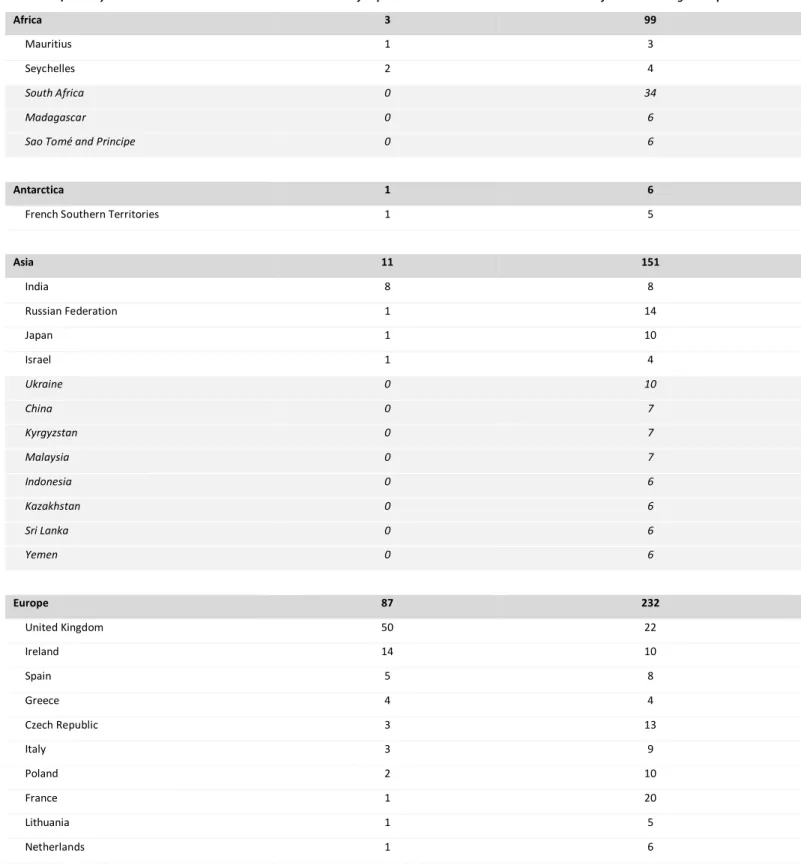
Table S2. Locations of impact observations. We list the 34 countries for which impact observations were available (white lines). To test whether impacts of ungulates were more often studied in countries with more introduced ungulate species (see Table S11), we added the numbers of introduced ungulate species per country (no re-introductions; extracted from Sheet 3 in Supp. 2). We completed the list with countries without impact observation, but with > 6 introduced ungulate species (grey lines and italic).

Continent/Country Number of impact observations Number of introduced ungulate species

Africa 3 99

Mauritius 1 3

Seychelles 2 4

South Africa 0 34

Madagascar 0 6

Sao Tomé and Principe 0 6

Antarctica 1 6

French Southern Territories 1 5

Asia 11 151

India 8 8

Russian Federation 1 14

Japan 1 10

Israel 1 4

Ukraine 0 10

China 0 7

Kyrgyzstan 0 7

Malaysia 0 7

Indonesia 0 6

Kazakhstan 0 6

Sri Lanka 0 6

Yemen 0 6

Europe 87 232

United Kingdom 50 22

Ireland 14 10

Spain 5 8

Greece 4 4

Czech Republic 3 13

Italy 3 9

Poland 2 10

France 1 20

Lithuania 1 5

Netherlands 1 6

(6)

Portugal 1 7

Germany 0 15

Sweden 0 10

Austria 0 8

Belgium 0 7

Slovakia 0 7

Denmark 0 6

Finland 0 6

Latvia 0 6

Slovenia 0 6

Switzerland 0 6

North and Central America 170 159

United States 119 33

Canada 41 16

Mexico 9 14

Saint Pierre and Miquelon 3 1

Saint Vincent and the Grenadines 1 1

Cuba 0 12

Antigua and Barbuda 0 7

Grenada 0 6

Haiti 0 6

Saint Kitts and Nevis 0 6

Oceania 123 110

New Zealand 61 18

Australia 49 21

Northern Mariana Islands 7 5

Fiji 3 5

New Caledonia 2 6

Papua New Guinea 1 11

Vanuatu 0 6

South America 47 104

Argentina 23 23

Ecuador 14 8

Brazil 6 9

Chile 2 10

Falkland Islands 2 6

Colombia 0 11

Peru 0 10

Bolivia 0 6

Venezuela 0 6

(7)

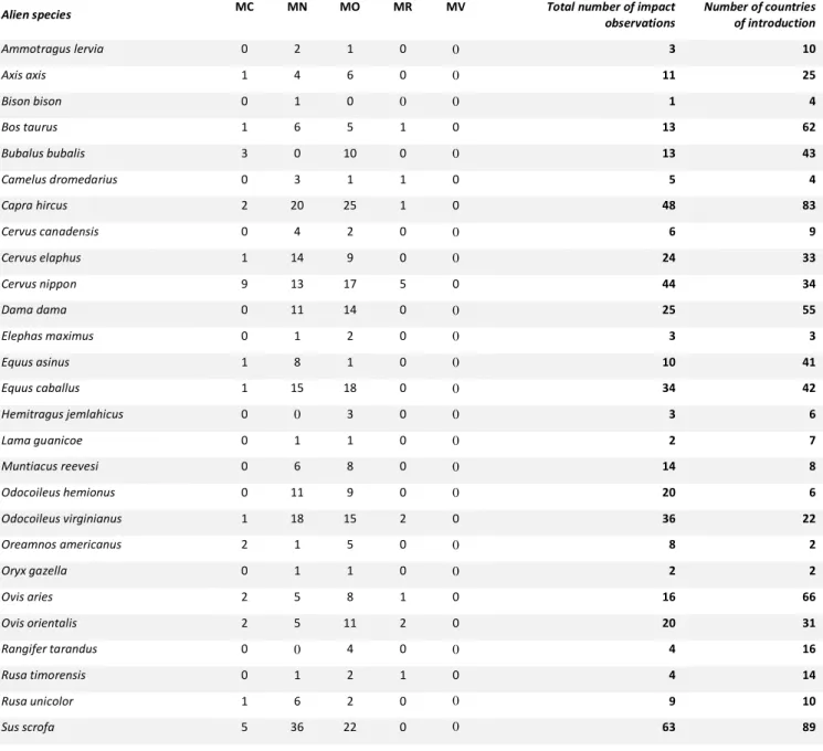
Table S3. Distribution of impact magnitudes per species. To test whether more widely introduced ungulates were more often studied (see Table S8), we added the numbers of countries each species has been introduced to (no re- introductions) (extracted from Sheet 3 in Supp. 2).

Alien species MC MN MO MR MV Total number of impact

observations

Number of countries of introduction

Ammotragus lervia 0 2 1 0 0 3 10

Axis axis 1 4 6 0 0 11 25

Bison bison 0 1 0 0 0 1 4

Bos taurus 1 6 5 1 0 13 62

Bubalus bubalis 3 0 10 0 0 13 43

Camelus dromedarius 0 3 1 1 0 5 4

Capra hircus 2 20 25 1 0 48 83

Cervus canadensis 0 4 2 0 0 6 9

Cervus elaphus 1 14 9 0 0 24 33

Cervus nippon 9 13 17 5 0 44 34

Dama dama 0 11 14 0 0 25 55

Elephas maximus 0 1 2 0 0 3 3

Equus asinus 1 8 1 0 0 10 41

Equus caballus 1 15 18 0 0 34 42

Hemitragus jemlahicus 0 0 3 0 0 3 6

Lama guanicoe 0 1 1 0 0 2 7

Muntiacus reevesi 0 6 8 0 0 14 8

Odocoileus hemionus 0 11 9 0 0 20 6

Odocoileus virginianus 1 18 15 2 0 36 22

Oreamnos americanus 2 1 5 0 0 8 2

Oryx gazella 0 1 1 0 0 2 2

Ovis aries 2 5 8 1 0 16 66

Ovis orientalis 2 5 11 2 0 20 31

Rangifer tarandus 0 0 4 0 0 4 16

Rusa timorensis 0 1 2 1 0 4 14

Rusa unicolor 1 6 2 0 0 9 10

Sus scrofa 5 36 22 0 0 63 89

(8)

Table S4. Impact magnitudes. Total numbers of impact observations classified in each impact magnitude.

Impact magnitude Count

Minimal Concern (MC) 32

Minor (MN) 193

Moderate (MO) 202

Major (MR) 14

Massive (MV) 0

441

Table S5. Confidence scores. Total numbers of impact observations classified in each impact magnitude and with each confidence score.

Confidence score MC MN MO MR MV Total

High 5 8 20 1 0 34

Medium 15 86 84 2 0 187

Low 12 99 98 11 0 220

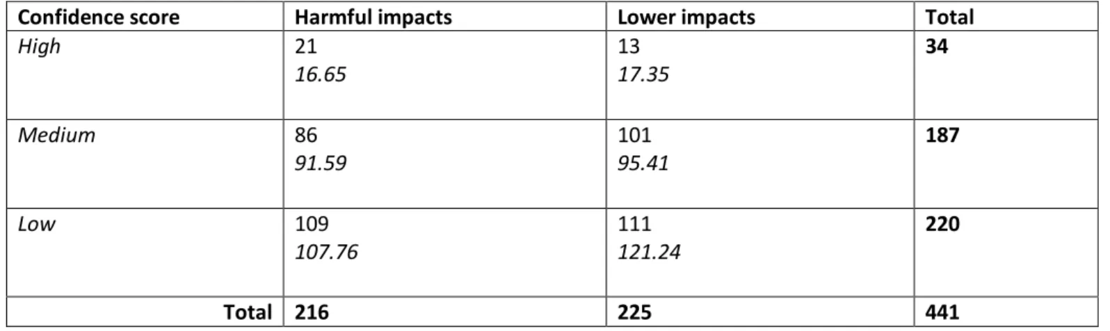
Table S6. Are harmful impacts associated with lower or higher confidence scores? Contingency table (Pearson’s Chi- squared test) showing observed and expected (in italic) numbers of harmful (MO, MR and MV) and lower (MC and MN) impacts by confidence score.

Confidence score Harmful impacts Lower impacts Total

High 21

16.65 13 17.35

34 Medium 86

91.59 101 95.41

187 Low 109

107.76 111 121.24

220 Total 216 225 441

X-squared = 2.92, parameter = 2, p = 0.23

(9)

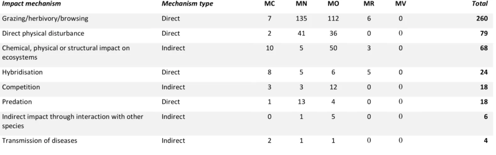
Table S7. Impact mechanisms. Total numbers of impact observations classified by impact magnitude and mechanism (some impact observations are recorded multiple times because they occurred through multiple mechanisms).

Impact mechanism Mechanism type MC MN MO MR MV Total

Grazing/herbivory/browsing Direct 7 135 112 6 0 260

Direct physical disturbance Direct 2 41 36 0 0 79

Chemical, physical or structural impact on ecosystems

Indirect 10 5 50 3 0 68

Hybridisation Direct 8 5 6 5 0 24

Competition Indirect 3 3 12 0 0 18

Predation Direct 1 13 4 0 0 18

Indirect impact through interaction with other species

Indirect 0 1 5 0 0 6

Transmission of diseases Indirect 2 1 1 0 0 4

Table S8. Are indirect mechanisms or direct mechanisms associated with higher impact magnitudes? We tested whether direct or indirect mechanisms were associated with harmful impacts on all 441 impact observations (see Sheet 4 in Supp. 2), except impact observations occurring through both direct and indirect mechanisms.

Model: glmer(harmful/lower impacts ~ direct/indirect mechanisms + (1|Region), family=binomial)

Estimate Std. Error p

Fixed effect: indirect mechanisms -1.41 0.31 < 0.001

Variance Std. Dev.

Random effect 1.07 1.03

AICc: 574.3; AICc of null model: 595.2 (∆AICc= 20.9)

Table S9. Impacted native species. Total numbers of impact observations classified in each impact magnitude, and in which animals or plants were affected. One impact observation is recorded twice because it affected both kingdoms.

Impacted kingdom MC MN MO MR MV Total

Animals 22 31 72 8 0 133

Plants 10 162 131 6 0 309

(10)

Table S10. Is native fauna or native flora associated with higher impact magnitudes? We tested whether native fauna or flora was associated with harmful impacts on all 441 impact observations (see Sheet 4 in Supp. 2), except the impact observation occurring on both native fauna and flora.

Model: glmer(harmful/lower impacts ~ native fauna/native flora + (1|Region), family=binomial)

Estimate Std. Error p

Fixed effect: native flora 0.73 0.25 0.005

Variance Std. Dev.

Random effect: Region 1.10 1.05

AICc: 594; AICc of null model: 600 (∆AICc= 6)

Table S11. Is the impact of ungulates more often studied in countries with more introductions? The numbers of impact observations and of introduced ungulate species for each country are given in the Table S2. We tested this on all 34 countries which had impact observations available, as well as on countries with no impact observations but at least six introduced ungulate species.

Model: lmer(log(number of impact observations for the country+1) ~ log(number of introduced ungulate species to the country+1) + (1|Continent))

Estimate Std. Error

Fixed effect 0.55 0.14

Variance Std. Dev.

Random effect: Continent 0.12 0.35

Residual 1.15 1.07

AICc: 208; AICc of null model: 218.4 (∆AICc= 10.4)

Figure S1. Caterpillar plot showing the variability in the increase of the number of impact observations per continent with the increase of introduced ungulate species.

Asia Africa Europe Antarctica South America North and Central America Oceania

-0.5 0.0 0.5

(11)

Table S12. Are more widely introduced species more studied? To test whether more widely introduced species were more studied, we tested, on all 66 ungulate species, whether the number of impact observations per species increased with the number of countries each species has been introduced to (see Table S1 for DD species and Table S3 for assessed species; DD species were assigned 0 impact observation).

Model: lm(log(number of impact observations per species+1) ~ scale(log(number of countries the species has been introduced to+1))

Estimate Std. Error p Residual

standard error

Adjusted R-squared F-statistic

1.10 0.09 < 0.001 0.78 on 64 DF 0.67 130.9 on 64 DF

AICc: 159; AICc of null model: 230.2 (∆AICc= 71.2)

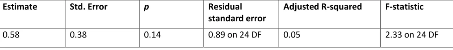
Table S13. Are species causing higher impacts more studied? We excluded DD species and the American bison (the only assessed species not causing higher impacts than MN impacts) and tested, on the remaining 26 species, whether the species having caused local extinctions (MR impacts) were more studied than species causing population declines (MO impacts) (see Table S3).

Model: lm(log(species’ total number of impact observations+1) ~ MO/MR impact)

Estimate Std. Error p Residual

standard error

Adjusted R-squared F-statistic

0.58 0.38 0.14 0.89 on 24 DF 0.05 2.33 on 24 DF

AICc: 72.7; AICc of null model: 72.5 (∆AICc= - 0.2)

Table S14. Are more widely introduced species causing higher impacts? We excluded DD species and the American bison (the only assessed species not causing higher impacts than MN impacts) and tested, on the remaining 26 species, whether the more widely introduced species were the ones causing higher impacts (local extinctions, MR impacts) (see Table S3).

Model: glm(MO/MR impact ~ scale(log(number of countries in which the species have been introduced+1), family=binomial)

Estimate Std. Error p Null deviance Residual deviance

0.72 0.46 0.12 32.1 on 25 DF 29.14 on 24 DF

AICc: 33.7; AICc of null model: 34.3 (∆AICc= 0.6)

(12)

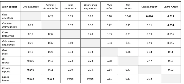
Table S15. Pairwise comparisons between the impact risks of the species classified in the Major category. When the impact risks of two species are significantly different from each other, they are shown in black and bold.

Alien species Ovis orientalis Camelus dromedarius

Rusa timorensis

Odocoileus virginianus

Ovis aries

Bos

taurus Cervus nippon Capra hircus Ovis

orientalis 0.29 0.19 0.20 0.10 0.064 0.046 0.013

Camelus

dromedarius 0.29 0.37 0.37 0.22 0.15 0.11 0.034

Rusa

timorensis 0.19 0.37 0.49 0.33 0.23 0.19 0.056

Odocoileus

virginianus 0.20 0.37 0.49 0.33 0.23 0.19 0.056

Ovis

aries 0.10 0.22 0.33 0.33 0.38 0.34 0.11

Bos

taurus 0.066 0.15 0.23 0.23 0.38 0.47 0.17

Cervus

nippon 0.046 0.11 0.19 0.19 0.34 0.47 0.12

Capra

hircus 0.013 0.034 0.056 0.056 0.11 0.17 0.12

(13)

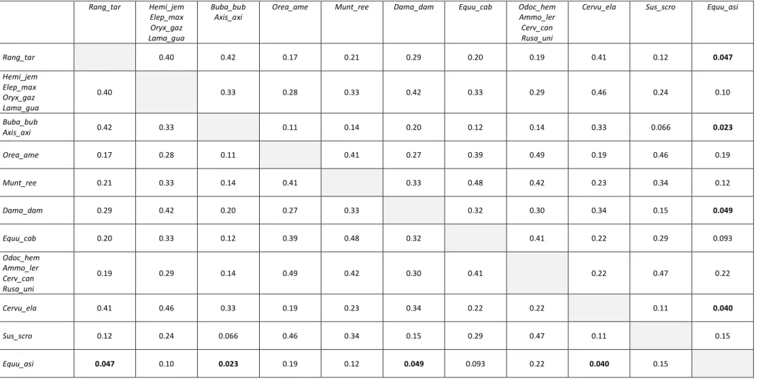
Table S16. Pairwise comparisons between the impact risks of the species classified in the Moderate category. When the impact risks of two species are significantly different from each other, they are shown in black and bold.

Rang_tar Hemi_jem Elep_max Oryx_gaz Lama_gua

Buba_bub Axis_axi

Orea_ame Munt_ree Dama_dam Equu_cab Odoc_hem

Ammo_ler Cerv_can Rusa_uni

Cervu_ela Sus_scro Equu_asi

Rang_tar 0.40 0.42 0.17 0.21 0.29 0.20 0.19 0.41 0.12 0.047

Hemi_jem Elep_max Oryx_gaz Lama_gua

0.40 0.33 0.28 0.33 0.42 0.33 0.29 0.46 0.24 0.10

Buba_bub

Axis_axi 0.42 0.33 0.11 0.14 0.20 0.12 0.14 0.33 0.066 0.023

Orea_ame 0.17 0.28 0.11 0.41 0.27 0.39 0.49 0.19 0.46 0.19

Munt_ree 0.21 0.33 0.14 0.41 0.33 0.48 0.42 0.23 0.34 0.12

Dama_dam 0.29 0.42 0.20 0.27 0.33 0.32 0.30 0.34 0.15 0.049

Equu_cab 0.20 0.33 0.12 0.39 0.48 0.32 0.41 0.22 0.29 0.093

Odoc_hem Ammo_ler Cerv_can Rusa_uni

0.19 0.29 0.14 0.49 0.42 0.30 0.41 0.22 0.47 0.22

Cervu_ela 0.41 0.46 0.33 0.19 0.23 0.34 0.22 0.22 0.11 0.040

Sus_scro 0.12 0.24 0.066 0.46 0.34 0.15 0.29 0.47 0.11 0.15

Equu_asi 0.047 0.10 0.023 0.19 0.12 0.049 0.093 0.22 0.040 0.15

(Rang_tar: Rangifer tarandus; Hemi_jem: Hemitragus jemlahicus; Elep_max: Elephas maximus; Oryx_gaz: Oryx gazella; Lama_gua: Lama guanicoe; Buba_bub: Bubalus bubalis; Axis_axi: Axis axis; Orea_ame: Oreamnos americanus; Munt_ree: Muntiacus reevesi; Dama_dam: Dama dama; Equu_cab: Equus caballus; Odoc_hem: Odocoileus hemionus; Ammo_ler: Ammotragus lervia;

Cerv_can : Cervus canadensis; Rusa_uni : Rusa unicolor; Cervu_ela : Cervus elaphus; Sus_scro : Sus scrofa; Equu_asi: Equus asinus)

(14)

Table S17. Comparison with the impacts of alien amphibians (Kumschick et al. 2017) and birds (Evans et al. 2016).

Contingency table (unconditional Exact functional test) showing observed and expected (in italic) numbers of harmful (MO, MR and MV) and lower (MC and MN) impacts by alien taxa.