Analysis of intermodulation interference to the instrument landing system

ANALYSIS OF INTERMODULATION INTERFERENCE

TO THE INSTRUMENT LANDING SYSTEM

by

YEANG, CHEN-PANG

B.S., National Taiwan University, Taipei, Taiwan June 1992

Submitted to the Department of Electrical Engineering and Computer Science in Partial Fulfillment of the Requirements for the Degree of

MASTER OF SCIENCE

at the

MASSACHUSETTS INSTITUTE OF TECHNOLOGY

January 1996

@

Massachusetts Institute of Technology 1996 All rights reserved

Signature of Author

Department of ElectricalYngineerii (and Corri. ter Science .January 18, 1996 Certified by

/

Certified by

e

(I

I A ,

Accepted by ..A•Ai.-USE CTS INS'I'U'TE" OF TECHNOLOGY

APR 1

1

1996

LIBRARIES

/#

Dr. Ying-Ching Eric Yang Thesis Supervisor

Professor Jin Au Kong Thesis Supervisor

S-Frederic R. Morgenthlaler Clhaima'an, )epar men t Conmmittee on Graduate Studeuts

.L

-t --`\I r-\

ANALYSIS OF INTERMODULATION INTERFERENCE

TO THE INSTRUMENT LANDING SYSTEM

by

Yeang, Chen-Pang

Submitted to the Department of Electrical Engineering and Computer Science on January 18, 1996 in partial fulfillment of the requirements for the degree of

Master of Science ABSTRACT

This thesis provides a model that could quantitatively evaluate intermodulation interference for the localizer receivers of instrument landing system. In this model a receiver is divided into frequency selection stage, which selects the desirable RF signal and converts it to IF; and baseband stage, which retrieves course deviation from the localizer baseband waveform. Both stages are characterized by a set of parameters. The parameters are inverted by matching simulation results with experimental data for standard interference conditions. The model is then used to predict the course deviation current under any given interference environment.

Thesis Supervisor: Jin Au Kong

Title: Professor of Electrical Engineering

Thesis Supervisor: Ying-Ching Eric Yang

Contents

Acknowledgment

...

7

List of Figures ... ....

... ...

11

List of Tables ...

...

... 13

Chapter 1 Introduction

15

1.1 Background ... 15

1.2 ILS Localizer Operating Principle ... 17

1.3 Types of Radio Interference to ILS ... 21

1.4 Overview of Problem and Methodology ... 23

Chapter 2 Generic Model for ILS Receiver

25

2.1 Localizer Receiver Architecture ... 25

2.2 Modeling of a Nonlinear Device ... ... ... 27

2.3 Modeling of Frequency Selection Stage ... ... 33

2.4 Modeling of Baseband Stage ... ... 44

Chapter 3 Model Synthesis

58

3. 1 Experiilllents for ILS Receiveri Inlterfeieilce(' ... 58

3.2 M odel S ,tlt llesis-Inlversioll of RIeceiverI lara• I I('ers ... tI ... ... ..61 3.3 Iive I '('ive s a 1 1 reshold C rves ... ... .(

Chapter 4 Simulation Results

74

4.1 Designing Future Receivers ... 74 4.2 Pure-Carrier Intermodulation Interference ... 78 4.3 Calculation of Course Deviation Current ... 81

Chapter 5 Conclusion

83

Acknowledgment

I wish to express my appreciation to my advisor Professor J. A. Kong, who provides me the chance to embark this study. His enthusiasm and kindness encourages the author of this thesis in many aspects.

I am deeply indebted to my research mentor, Dr. Eric Y. Yang. He gave me a lot of very precious guides and suggestions from shaping research scheme to conducting detailed theorization and simulation as well as writing a technical text. In a sense I am enlightened by him. I am also grateful to Dr. Robert T. Shin and Dr. A. Jordan for their direction on me to the methodology of scientific research.

I wish to thank Mr. Yan Zhang, my research partner. Some of the important ideas in this thesis were initiated by him. His warmth and diligence prove him a best research partner. I also wish to thank my senior Mr. Chih-Chien Hsu. He gave me a lot of help in familiarity with computers. My senior Shih-En Shih and my friend Tza-Jing Gung were the ones I can always count on. I would also like to thank them for their spiritual support. I am very fortunate to be surround with excellent persons in Professor Kong's group, Dr. Kung-Hau Ding, Dr. Jean-Claude Souyris, Dr. Joel Johnson, Mr. Jung Yan, other colleagues and our secretary Ms. Kit-Wali Lai.

" You don't want to become Buddha, nor do you want to learn alchemy "

Said the Master, " Then the only thing I can teach you is Magic "

" Gee! ", the Monkey starts to contemplate

" I heard his 108 Varieties are pretty fantastic, can I try them ? "

List of Figures

1.1 Instrument Landing System ... ... 19

1.2 ILS operating principle ... ... 20

2.1 ILS receiver configuration ... . 26

2.2 Typical nonlinear input/output relationship ... 29

2.3 RF-section block diagram ... ... ... 34

2.4 Block diagram of a balanced mixer ... 37

2.5 Sixth-order Chebyshev filter ... 40

2.6 IF-section block diagram ... 40

2.7a Configuration of AGC ... ... 43

2.7b Procedures for AGC simulation ... 43

2.8a FM power spectrum. The 20-dB bandwidth is 64 KHz ... 47

2.81) M odeled FM power spectrum ... 47

2.9 Envelope detector circuit ... ... 50

2.10 IF and baseband noise spectrum (one side) ... 54

2.11 CDI output based on simulated and approximate(d clnvelopc detector ... 57

2.12 CI)I imean and standard deviation ... ... 57

3.2 FAA intermodulation threshold test results ... 62

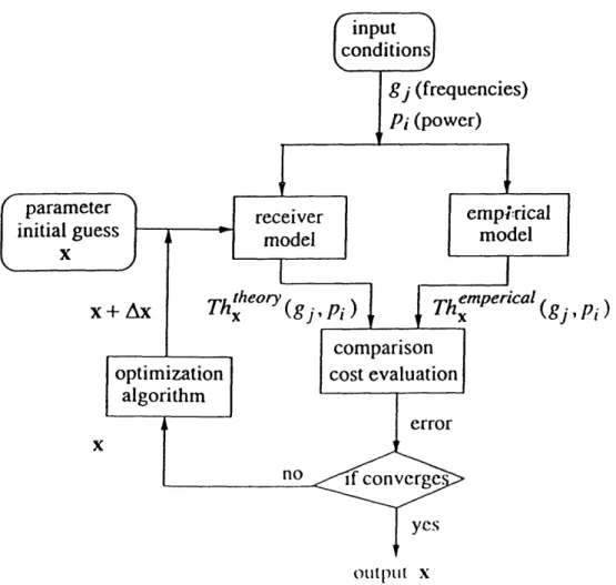
3.3 Parameter inversion procedures ... ... 68

3.4 Inverted AAM RF pre-filter response ... 71

3.5 Inverted ITU RF pre-filter response ... 71

3.6 AAM two-frequency B1 curves ... 72

3.7 AAM three-frequency B1 curves ... 72

3.8 ITU two-frequency B1 curves ... ... 73

3.9 ITU three-frequency B1 curves ... 73

4.1 Inverted ICAO RF pre-filter response ... 76

4.2 ICAO two-frequency B1 curves ... 77

4.3 ICAO three-frequency B131 curves ... 77

4.4 Comparison of pure-carrier interference with FM interference: AAM model ... 79

4.5 Comparison of pure-carrier interference with FM interference: ITU model ... 79

4.6 Comparison of pure-carrier interference with FM interference: ICAO model ... 80

4.7 Specification of over-threshold, threshold and under-threshold conditions ... 81

4.8 CDI distribution: over-threshold ... ... 82

4.9 CDI distribution: threshold ... 82

List of Tables

2.1 Simulated CDI for zero-noise conditions ... ... 56

3.1 Intermodulation frequencies (two frequencies) ... 70

3.2 Intermodulation frequencies (three frequencies) ... 70

3.3 Inverted receiver parameters ... 70

Chapter 1

Introduction

1.1 BACKGROUND

For the past few decades, Instrument Landing System (ILS) has been used to provide precision landing aid for aircraft during the period of low visibility. The operation of instrument landing system depends on the communication of radio signals between ground-based transmitters and airborne receivers. The ILS radio signals provide information of the aircraft course deviation, height and distance from the landing spot. The messages retrieved from airborne sensor can be fed into the aircraft control system. Newly developed landing systems such as Microwave Landing System (MLS) and Global Positioning System (GPS) adopt different spectrum regions, system architecture or coding characteristics; but they also rely on propagation of EM waves to get information of the airplane.

Chapter 1 Introduction

Since its invention ILS has worked well for the airports around the world without serious incidence. However, increasingly hostile radio environment around the airports due to urban development has gradually threatened its performance. Larger number of airport within a region makes it difficult to find ILS frequencies for different runways without running into interfering with other radio navigation systems. Buildings construction around the airport increases the opportunity of multipath interference to ILS radio signals. In addition, growth of FM stations, Industrial-Scientific-Medical equipment (ISM) and other instruments which radiate frequencies adjacent to ILS spectrum region also aggravates interference potential. The affore mentioned new systems is under consideration but the civil aviation authorities also made significant effort to alleviate those existing problems. The new landing systems utilizing different frequency band and signal processing schemes, such as MLS and GPS, have been developed. Before the transition to new systems has completed, however, the principal system is still ILS. Therefore the evaluation and improvement of ILS interference immunity are very important.

An appropriate way to conduct the evaluation of automatic landing system is to do statistical simulation on the landing process under realistic radio environment. The statistical parameters obtained from simulation such as failure rate are the basis for performance evaluation. In order to complete this simulation a theoretical ILS receiver model studying at the effect of radio interference is necessary. It is known that ILS interference comes from different types of mechanisms. In this thesis we choose intermodulation interference to be tile target of analysis. It is because the spectrum range of a specific ILS subsystem: localizer (108.1 MHz to 111.95 MHz) is very close to FM broadcast band (88.1 MHz to 107.9 MHz), FM power (1 to 100 KW) is much larger than localizer power (15W), and therefore FM broadcasting signals are capable of driving the receiver into nonlinear region to generate interimodulation components. The fi-eeuencies of low-order internlmodulation components, which often posses larger power, are close to localizer band. Apparently FM interlnodlllation interferenice is a non-negligible problem for ILS localizer.

1.2 ILS Localizer Operating Principle

The purpose of this thesis is to present an analysis of intermodulation interference on ILS localizer receiver. A generic model based on ILS circuit configuration is developed to cover the general population of receivers in service. This model contains the frequency selection part which include sections from RF to IF, and baseband signal processing part which include sections from IF envelope detector to output. The output error as a function of interfering frequencies is simulated and compared with empirical results. In order to invert appropriate receiver parameters an optimization technique is adopted to fit experimental results. This generic model is then used to extrapolate system response in other radio environments.

1.2 ILS LOCALIZER OPERATING PRINCIPLE

Instrument landing system (ILS) consists of three subsystems: localizer trans-mitter for azimuth guidance, glide slope transtrans-mitter for vertical guidance and marker beacons or distance measuring equipment (DME) for distance-to-threshold guidance. The placement of ground systems and rough sketch of operating principles are indi-cated in Figure 1.1. The localizer frequencies span from 108.1 to 111.95 MHz. There are altogether 40 channels, allocated at odd 100 KHz and 50 KHz frequencies. The glide slope frequencies span from 328.6 to 335 MHz. The DME frequencies span from 960 to 1215 MHz. These three components are tied together, so there are 40 channels in glide slope and DME as well [10].

ILS localizer provides the measure of azimuth deviation of airplane from the runway center line. Its operating principle is illustrated in Figure 1.2. The ground system contains a set of transmitting antenna arrays near the end of runway. The transimitted signal has two components, which are 90 IHz and 150 Hz respectively,

anmll)lit ucle-nmlodulate(d with localizer carrier frequency flo( . The arlrays are arranged such that. the lbeamln patterns for the two Imodulated signals point to differeint sides of the runlway and are symmmietric. Thus along the runway centerline, their signal

Chapter 1 Introduction

strength are equal. The field strengths in front of both antenna sets are of the same power and modulation index, i.e. Aoc[1

+

m cos(2r 90t)] cos(27rfloct) and AT [1 + mcos(2r- 150t)] cos(27rfloct). The airborne receiver tuned at same localizer channel floc detects a combination of 90 Hz and 150 Hz signals ARx[1 + m9 0 cos(27r

90t) + m150 cos(2r - 150t)] cos(27rfloct). As indicated in Figure 1.2, m90 and m150

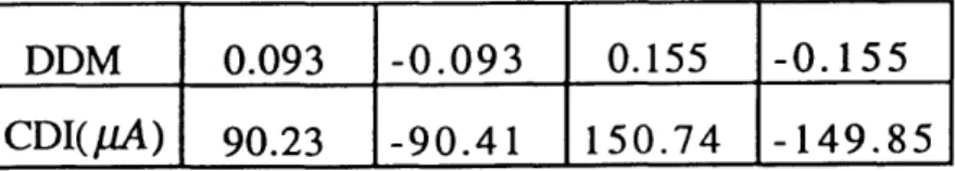
are functions of aircraft angular deviation 0. The way they are related to 0 depends on the shape of antenna beam pattern. With a narrow range of 0, usually between -20 and 20, the difference in depth of modulation DDM), m9g(0) - m1 50(0), is approximately proportional to 0. The numerical bound of modulation indices m90

and m150 can be calculated on the basis of localizer antenna beam pattern and modulation index of transmitted AM. Within the two-degree range the modulation indices are bounded within 0.2 0.0775. A localizer receiver outputs +150, A course deviation current when the angular deviation is +20 , and -150pi A current when the angular deviation is -2 . The function of localizer receiver is to retrieve DDM from the input signal

al _-- go( -eAI.( _{. ... I --. ac(}4(AAAI(4(A S (Or(eHKO. Ka 4 %-40 4%Xf "- A -AC& CA o AA CA 7C~ (i-u -•u VXtrAO rf g . S- 1 I 1 SJ:O c -CkC(ffz

Figl. _{Ilistrliiumint Landiing System f(2}

a

a

Chapter 1 Introduction

Localizer beam pattern.:

A + mingo (0) cos(2 r90 t) ]cos(2

7f,,t)

landing reg

runway center

A

[I

+

ms

o

(O) cos(2

rl50t)]

cos(2

xf,,.t)

ILS localizer receiver:

:urrent

Angular dependence of DDM:

0.155

-2

mr,.so

₎

+2

-0.155

1.3 Types of Radio Interference to ILS

1.3 TYPES OF RADIO INTERFERENCE TO ILS

Several physical mechanisms have been identified as possible causes of radio in-terference to ILS. They are divided into four classes by the International Telecommu-nication Union (ITU): Al, A2, B2 and Bi. Al is in-band interference. It refers to the condition when the input noise spectrum directly overlaps with localizer passband such that the amplitude of 90 Hz and 150 Hz subcarriers are changed. The band to cause Al interference is very narrow: centered at the operating localizer frequency it spans the width of localizer passband (several hundreds Hz). Since no other radio communication than ILS localizer is allowed within 108.1 MHz to 111.95 MHz, the likely source of interference is the harmonics of transmitters at other bands.

A2 covers the general adjacent-band interference. It is generated by the noise with spectrum not exactly in but very close to localizer band such that part of it falls in the receiver passband. The noise cannot be completely got rid of before receiver baseband so the amplitudes of 90 Hz and 150 Hz subcarriers are changed accordingly. A2 happens only when both localizer channel and interference spectrum are very close to 108.1 MHz, for example, localizer channel 108.1 MHz and FM channel 107.9 MHz. When the radio frequency is far away from the desired receiver frequency but causes interference the mechanism is classified as B2. It occurs when the input noise power level is relatively high. Because of the high input power the mechanism responsible for B2 is probably receiver nonlinearity.

The type of interference dealt in this thesis is B1 - intermodulation interference.

A l, A2 and B2 can be induced by one frequency, but B2 should be induced by two or more. Interniodulation is also the product of receiver nonlinearity. For a nonlinear systemlll, the out)plut includes not only those frequencies which are present in input excitation, b)ut also numiblers of harInon(ics which are the coiimbinations of the input, fre ueilcies. Interlnodulation interference to the receiver occurs when the receiver is d(rivell inIto _{a nonlinear region of operation by high-powered signal} such that, the

22 Chapter 1 Introduction

output. For the intermodulation to occur, at least two signals need to be present. And the harmonics are linear combinations of input frequencies. For example, if the input of a nonlinear device contains two frequencies fl and f2, then the second-order intermodulation components occur at fl + f2 and fl - f2, the third-order

intermodulation components occur at 2_{fl + f2,} 2_{fl - f2, 2f2 + fl and 2f2 - fl ,} and so on. Even if all the interfering frequencies lie out of the receiver passband, their intermodulation components can fall right at the desired frequency. The proximity of FM broadcasting frequencies to ILS localizer band makes localizer receiver susceptible to FM-generated intermodulation interference.

1.4 Overview of Problem and Methodology

1.4 OVERVIEW OF PROBLEM AND METHODOLOGY

The calculation of intermodulation products from multiple input frequencies has been known to be a tedious problem [11] [28]. In the past half century intensive study of intermodulation interference in communication and broadcasting technology have been conducted. Some of the most distinguishable cases of interest can be found in wireless communication circuits [6] [8] [13] [14] [22] and cable TV circuits [1] [4] [18] [22]. Most literature put emphasis on analyzing intermodulation effect of individual nonlinear device, for example, RF amplifiers and mixers. However, quantitative study of intermodulation on the whole system has been lacking. The latter is important for analyzing the interaction between RF systems and control systems, as in the case of ILS-driven aircraft automatic landing system. Only when we construct the model of whole system on the basis of available empirical data can we achieve this goal.

Out of this concern, the aviation community has studied ILS interference problem through a series of bench experiments on different kinds of operational receivers. These experiments consist of measuring the "threshold" of interfering power as a function of frequency under Al, A2/B2 and B1 conditions. Regression formula derived from the performance of typical receivers were derived. These empirical formula is important for radio environment evaluation since they specify the cut-off level at which interfering power is considered intolerable.

However, the regression curves specify the threshold conditions only. They do not provide the information of ILS response to the cases under or above the threshold conditions. Thlis information is important for the overall simulation of aircraft landing process. Therefore a receiver simulation model is necessary. Since it is impossible to run tihe detailed simulation for all kinds of ILS receivers on the miarket, we develotp a

"gelieric" M11odel based o011 tihe regressioll formula. The ilmethodology is described

as follows: (1) Based oil real operations of ILS receivers and certain accept able assulmill)tiolls, a simplified llatlienmatical nmodel is derived. This niodel is characterized b)y a set, of parammeters. (2) Thie paramneter values are inverted(l fronil a set of regressionl

Chapter 1 Introduction

curves. In this thesis two-frequency B1 curves are chosen as the objective to be fitted. (3) Apply the model to other conditions and compare the simulation results with new regression curves to verify the consistency of the generic receiver model.

The following chapters are arranged as follows: Chapter two is the detailed description of mathematical model. It includes frequency selection stage which converts RF into IF signal and baseband stage which extracts course deviation current from IF signal. Chapter three is the synthesis of receiver model with respect to empirical results. It contains the experimental procedures for ILS B1 test, regression formula for experimental results, inversion procedures for retrieving values of parameters, the values of receiver parameters inverted from regression formula of two-frequency intermodulation, and simulated threshold curves. Chapter four extends current model to different interference conditions. It includes the extrapolation of future-standard ILS receivers, simulation on pure-carrier intermodulation interference and CDI calculation under non-threshold interference conditions.

2.1 Localizer Receiver Architecture

Chapter 2

Generic Model for ILS Receiver

2.1 LOCALIZER RECEIVER ARCHITECTURE

The configuration of localizer receiver is in Figure 2.1. There are two principal stages in the receiver. The first stage, or frequency selection stage, recovers baseband signal from its amplitude-modulated form. It functions like a regular AM receiver, converting RF input into baseband output. At the very front an RF section filters and amplifies the input. Its output is fed into a mixer which multiplies the incoming RF signal by a local oscillator carrier to down-convert the operating frequency to IF. The IF signal is filtered and amplified in IF section. After IF an envelope detector is followed to detect the amplitude of IF output. Baseband signal is retrieved at the output of envelope detector. In additional to RF, mixer and IF, Automatic Gain Control (AGC) which confines the output power level of frequency selection stage within a narrow range is also incorporated.

Chapter 2 Generic Model for ILS Receiver

Generic Model for ILS Receivers

RF in

CDI

Frequency Selection Stage

I

Baseband Stage

2.2 Modeling of a Nonlinear Device

The second stage converts processed IF signal into Course Deviation Indicator (CDI) current. We shall call it baseband stage. Baseband signal is splitted into two paths: the first one contains a 90 Hz-centered bandpass filter and an envelope detector, the second one contains an 150 HZ-centered bandpass filter and an envelope detector. The output of the two paths are fed into a differential amplifier to get the course deviation current. Among all the sections IF envelope detector is the interface between the frequency selection stage and the baseband stage. In the following paragraphs IF envelope detector is attributed as a part of baseband stage.

A generic receiver model is built by linking all the models of function blocks in Figure 2.1 and cascading them together. The following sections will discuss the construction of frequency-selection-stage model and baseband-stage model in more detail. The modeling of a single nonlinear device is necessary before starting a macroscopic consideration.

2.2 MODELING OF A NONLINEAR DEVICE

Intermodulation interference is the result of receiver nonlinearity. For modeling purpose, we consider a nonlinear system S with one input x(t) and one output

y(t). Similar to the way a linear system is represented by an impulse response

h(t), a nonlinear system will be represented by a series of impulse responses hl (t), hI2(tl, t2), h3(t1 t2, t3), .... such that

Chapter 2 Generic Model for ILS Receiver

The form of (2.2.1) is called the Volterra-series representation [27] [29]. This representation takes into account not only high-order terms due to nonlinearity but also the temporal variation. In general y(t) cannot be expanded into a power series of x(t) but is a integral-transform type series with which transfer functions hl(t),

112(tl, t2), .... are involved.

Rather than sticking to this rigorous but complicated proposition, the thesis assumed that output y(t) is a functional of input x(t).

y(t) = F(x(t)) (2.2.2)

This assumption is correct if the operating amplitude and frequency are within reasonable regions. For example, to the first-order approximation the capacitive effect of a PN junction could be ignored and diode current (output) Id(t) is related to diode voltage Vd(t) by the formula Id(t) = Io(exp(Vd(t)/VT) - 1). The source of ILS receiver nonlinearity is mainly amplifier. It is well known that temporal variation is secondary in nonlinear amplifiers like FET or BJT. Modeling i/o relationship as a functional is a valid approximation. If y is a function of x then it could be expanded into a power series of x:

y =

Kxz

(2.2.3)

i=1

How many terms should we keep in order to cover the dominant nonlinear effect depends on the function itself and input amplitude. For a nonlinear amplifier, the in)put/output relationship usually resembles a curve like the one in Figure 2.2.

2.2 Modeling of a Nonlinear Device

y

Fig2.2 Typical nonlinear input/output relationship

The operational region, could be approximated by a low-order polynomial. If input amplitude is not high enough to drive output into saturation, then it is valid to model a nonlinear device as a low-order polynomial:

N

yx Kix i (2.2.4)

i=l

This thesis concentrates on the third-order approximation. For the case of FM (88.1 to 107.9 MHz) intermodulation interference on ILS localizer (108.1 to 111.95 MHz) the second-order term K2x2 generates harmonics far beyond localizer frequency (either floc - fFM or floc + fFM ), so it is sufficient to keep only two

terms: linear and the third-order:

y K1x +1 +- K3x3 (2.2.5)

Intermodulation interference generated by a single nonlinear device could be calculated bly using this model. Consider the case where N interfering components

Ai cos(27rft -4- 0i) along with a desired component Ao0 os(27rf0t) enter the device:

N

x(t) = A0 cos(2 7rf 0t) + t Ai cos(2T fit + 4i) (2.2.6)

Chapter 2 Generic Model for ILS Receiver

The output y(t) = Kjx(t) + K3x(t)3 contains linear part x(t) (see (2.2.6)), and nonlinear part x(t)3: N A3 =(t)3 - [cos(3(2wrfit i=O A2A + 3[ 2 cos(27rfjt O<i<j<N A2A + 4 cos(27r(2fi

+

cos(2~(2fi

A2 A-+ 4 cos(27r(2fj

+ 0i)) + 3 cos(27rfit + 0i)]

A2Ai

+ j) + 2 cos(21rfit +

+ fj)t + 20i + 0j) - fj)t + 20i - j) + fi)t + 20j + 0i) A2Ai

+ • cos(2r(2fj - fi)t + 20j - i)]

4

+ Oj

O<i<j<k<N 2AiAjAk[cos(2r(fi + fj + fk)t + Pi

+ cos(27r(-fi + fj + fk)t - €i +

±j

+ €k)

+ cos(27(fi - fj + fk)t + 0i - ±j + Ok) + cos(27r(fi + fj - fk)t + ¢i + Oj - k)0]

where i = 0 represents desired signal.

The output sinusoidal components with frequency fJ are:

+ Oj + ¢k)

2.2 Modeling of a Nonlinear Device

(a) K1Ao cos(2rf0ot)

(b) 4K3A03 cos(27rf 0t)

(c)

EN_

1

3K

3

AoA

cos(27rf

0t)

(d) 2f-fj=fo •A Ajcos(27r(2fi - fi)t + 20i - j)

(e) Efi+fj-fk=f AiAjAk cos(2r(fi + fj - fk)t + €i + j - 46k)

(a) is the linear term. (b) is generated by third-order intermodulation of localizer frequency with itself, fo - f0 + f . It is named 'self-modulation' component [23]. (c) is generated by third-order intermodulation of localizer frequency with one interfering frequency, fi-fi+fo. It is named 'cross-modulation' components [22]. (d) and (e) are generated by third-order intermodulation of two and three interfering frequencies. (b) and (c) have exactly the same spectra as localizer signal (a) since no qi(t) appears in the phases. They essentially modifies the amplitude of localizer signal but eventually would not effect the output CDI value. So (b) and (c) can be seen as parts of signal. Combination of (d) and (e) is third-order intermodulation interference generated by device nonlinearity. To summarize, the signal part at output is

[KIA + K3A0 +

3

A0A 2]cos(27rfot)

i=1

And the interference part is

3 K3A Aj cos(27rf0t + 25i - j)+

2

ffi-j =ffo

2 I3AAAk cos(27rfot + 5i + cj - Ok)

Chapter 2 Generic Model for ILS Receiver

Let the summation of these two parts equal to y(t). Its total amplitude depends on phases 41, 2,.... In the case of ILS localizer, the most serious source of intermodulation interference is FM broadcasting. The phases of FM carriers are the messages to be transmitted, therefore they are functions of time. In general they are stochastic processes and uncorrelated with one another. The ensemble average power of y(t) is the summation of coherent (signal) power and incoherent (interference) power:

3N 2

2 < y(t)2 >= [K1AO + 4K3Ao3 + j -K 3AoA?]

i=1

+ 29 2•A + 9K2A2A2 (2.2.8)

163 4 3 i j k(2.2

2fi-f=fo _{fi+fj-fk fo}

Taking the square root of average power to be the effective amplitude, the fo

component at the output becomes

y(t) < y(t)2 > cos(27rfot + q) (2.2.9)

Equation (2.2.8) and (2.2.9) apply to other frequencies as well. They provide the formulation to calculate a nonlinear device's output.

2.3 Modeling of Frequency Selection Stage

2.3 MODELING OF FREQUENCY SELECTION STAGE

In a receiver the RF signal should be processed and converted into baseband signal. This is done by frequency selection stage. As indicated in Figure 2.1, the frequency selection stage consists of RF, mixer, and IF sections, like a typical AM receiver. A realistic AM receiver may have more than one IF section. In our simplified model only one IF section is presented. This should not, however, affect the simulation results significantly.

In the frequency selection stage model we also only need to treat either localizer signal or undesired FM interference at a specific broadcasting frequency like a pure carrier, and leave those detailed phase terms to the baseband signal processing stage. For the localizer component, we take the root mean square of the slowly-varying envelope as effective amplitude:

A"n[1 + mgg cos(27r 90t) + m1 50 cos(27r 150t)] .A [1 + O.5m 0 + 0.5m250

(2.3.1)

The value of modulation index m90 and m1 5 0 is between 0.2775 and 0.1125 in the operation range of localizer. Under most cases it is valid to assume m_{9 0} 1. m1_{1 50}

0.2. Therefore the effective amplitude can be further approximated:

Aloc[1 + m90 cos(2r - 90t) + m15 0 cos(27r - 150t)] A AlocV/i.0i (2.3.2)

Instead of having a temporally varying amplitude, the FM interference contains a tellmporally varying phase. To treat it as a pure carrier, we assume the slowly varying phase flinc:tion is approximately a constant:

Chapter 2 Generic Model for ILS Receiver

The pure-carrier approximation is valid since either the localizer signal bandwidth (no more than several KHz) or the FM bandwidth (64 KHz for standard test condition, see [20]) is much narrower than RF (88 to 112 MHz), RF bandwidth (several MHz) and IF center frequency (5 to 30 MHz).

2.3.1 RF Section

Xin

Xout

Fig2.3 RF-section block diagram

Figure 2.3 is a RF-section block diagram. It contains an RF pre-filter, an amplifier and a post-filter. A pre-filter is often a tuned LC circuit or other equivalent passive bandpass filter. It can be characterized by a frequency response function

H"F(f) =

Hr

(f)I exp(i RreF(f)) For an input x(t) = N1 A i cos(2 7rfit+ i), the output of pre-filter is y(t) =

E

₁ Hp

Fi)ji

cos(2rfit+

4

())

Typically

IHRrF(f)I

peaks around the center frequency fc and drops monotonically on both sides. The center frequency fc is usually tunable with localizer frequency floc. The filter transfer function is usually normalized such that the peak value is unity. Here we adopt the same convention to split RF pre-filter characteristics into two parameters: normalized filter response and front-end gain:

lHRFold(f) HI. (f) (2.3.4) where JIHF (fc) = 1.

The RF post-filter is modeled exactly the same way as pre-filter excCp)t with a (different frequency response Hp (f) and normalization constant AI "

2.3 Modeling of Frequency Selection Stage

The RF amplifier is often a transistor device such as field effect transistor (FET). The effect of temporal variation in this kind of device is considered secondary within the operating frequency range. However its nonlinear effect cannot be ignored. The model described in Section 2.2 could apply here. From experiments it is observed that nonlinearity of RF amplifier K3/K 1 varies with different input power levels [7]. In this thesis, third-order nonlinearity is specified at few discrete input power levels.

Given Hprelf\ Apre KK post post

Given HrF( f) , A RF K3 , K1, HRF (f , RF and input amplitude for

each frequency component, the amplitude of each frequency at RF output could be evaluated. Ideally a pre-filter is very selective so that all interference other than localizer frequency is suppressed. But it is difficult to implement such a filter. Separation between localizer and FM is less than 200 KHz, a bandwidth RF filters could hardly achieve. Thus significant amount of energy in the FM signal can pass the filter and cause intermodulation interference. The interference amplitude is a function of pre-filter response at input FM frequencies Hre(f1), H•' .e2). .If RF pre-filter and post-filter cannot suppress interference well, then nonlinearity after RF section has to be considered. In this case mixer would produce non-negligible intermodulation interference.

Chapter 2 Generic Model for ILS Receiver

2.3.2 Mixer

Mixer is also a nonlinear device. Unlike an amplifier, a mixer has two input: one is from RF section and the other is from local oscillator. Ideally the output of a mixer is the product of two inputs. Without interference, the RF-section output is pure localizer signal x(t) = AOR F cos(21rfloct) . The local oscillator output is a pure

sinusoidal wave xosc(t) = Aosc cos(2irfosct + Oosc) , where the frequency difference

between both is IF,

Ifosc -

flocl

= fIF - fosc could be larger or smaller than floc.

In the model we assume a superheterodyne receiver, i.e. fosc - floc = !IF . Thus

the ideal mixer output y(t) is

y(t) = x(t) -. osc(t) = AORFAosc/2[cos(21r(fosc +

floc)t

+ 0osc)

+ cos(27r(fosc - floc)t + qosc)] (2.3.5)

The first term, which is far above the IF band, can be removed by the IF filter.

A real mixer contains more terms than (2.3.5). We consider the following approximation model represented by the fourth-order Taylor series expansion over two variables: Generally a mixer is a nonlinear 'three-port'. The output y is a function of x and Xosc. It can be expanded into a Tayler series

y

= f(z,

Xosc)

=

f(x

o, xzosc)

+

)o+

o(

)oX

sc

0

(

2

+ (

2

_:2o+

++s

xxo

+

_+z

(o 2

f

f

_os

ta

3

_f

₍

_af

_j3

.

K

₃

_03f

_{XXsc +)}

o 0 _{(oS) o 0)} S( f x4 0f "3 1 9 2 2

+4(

+4

x

o6

+

,

x,

....

OSC

2.3 Modeling of Frequency Selection Stage

+4

04jf XX

+o3sc

t-

ox sc + H.O.T.

(2.3.6)

where

O

represents operating point, e.g.

()

° means

the value of function (_-)

at the operating point (x, Xosc) = (x0, Isc) . H.O.T. refers to high-order terms.

It is obvious that in (2.3.6) the odd-order terms do not lie in the IF passband provided input frequencies are not far from RF. Unlike a nonlinear amplifier, the relevant intermodulation components of a mixer are second-order, fourth-order,... and so on. XXosc provides desired localizer signal, x2 and x2sc generate baseband frequencies and fourth order plays the role of amplifier's third order. For example, if there are two interfering frequencies fi f2 satisfying 2fl - f2 = floc, then X3_Xosc

would produce intermodulation term with frequency fosc - fl - fi + f2 which is exactly equal to fIF (fosc - floc)"

Eight terms in (2.3.6) should be kept (second and fourth order) to include both linear and third-order intermodulation effects. This means generally a mixer is characterized by eight coefficients, which makes the model more complicated. We shall consider a simpler but realistic situation, i.e. the balanced mixer. The balanced mixer uses two symmetric nonlinear devices to eliminate the first-order components. Its configuration is in Figure 2.4.

-1

X

XOSC )

out

XOSC )

Chapter 2 Generic Model for ILS Receiver

The output of a balanced mixer y(t) is a nonlinear function of x and Xosc with form:

y = g(x + Xosc) - g(x - Xosc) = g(1)(o) • 2xosc + g(2)(o) - 2xxosc

+1/3g(3)(o) - (3x2Xosc + Z3sc) + 1/3g(4)(o) (x3Xosc + X3scx) + H.O.T. (2.3.7)

Among the lower-order terms in (2.3.7) the ones capable of generating IF are

g(2)(o) 2zxosc and 1/3g(4)(o). (x3Xosc+ X3scz). Let 2g(2)(o) = K2 , 1/3g(4)(o)=

K4 , x = N= An cos(2rfnt + On) and Xosc = Aosc cos(2irfosct + osc) . Substitute into (2.3.7) and get rid of out-of-IF-band components, the resultant y would be

N

y = (1/2K₂Aosc + 3/8K4Aosc3) E An cos(27r(fosc - fn)t + qosc - On)+

n=1

M

1/2K4Aosc E Bm cos(27r(fosc - fm)t + Oosc - Om) (2.3.8)

m=1

where Em=1 Bm cos(2r fmt + Om) = N An cos(27rfnt + On)3

Therefore the operation of balanced mixer resembles that of a nonlinear amplifier with linear coefficient 1/2K2Aos c+3/8K4Aosc3 and third-order nonlinear coefficient

1/2K4Aosc, except that every sinusoid contains a phase difference qosc. Only two coefficients are required to characterize a balanced mixer.

2.3 Modeling of Frequency Selection Stage

2.3.3 IF Section

Generally IF section is similar to RF section, but they differ from each other in several aspects. The IF filter is much more selective than the RF filter. In the case of ILS localizer the 3-dB bandwidth is usually no more than 100 KHz, and at least 60 to 80 dB attenuation would be reached for the FM interference. The IF amplifier can also achieve higher gain than is possible for RF amplifier. A common IF circuit consists of a highly selective crystal filter followed by a series of cascading amplifiers. The crystal filter corresponds to IF pre-filter. Typically IF filters used in localizer receivers are implemented as Chebyshev filters having order 6, 8 or 10 [26]. For the worst-case consideration, sixth-order Chebyshev filter is used in receiver model. It has the magnitude response:

1H

e

_f1

_{+ 1.512T12(f)}

(2.3.9)

where T1(f) = 4TO3(f) - 3TO(f), To(f) = B f 2)

The frequency response of sixth-order Chebyshev filter is demonstrated in Figure

2.5.

The amplifier set is not only a nonlinear device but also contains RC circuits that serve as filters. It corresponds to IF amplifier and IF post-filter. Notice that IF amplifier may perform a better linearity either because more linear device could be used (e.g. BJT) or more delicate design could be applied to reduce nolincarity (e.g. log amplifier) under lower frequency range. Because IF pre-filter is highly selective, illtermnodulatioIL at tie IF amlplifier is negligible unless incoming FM interference is extremlnely large. In our receiver imodel IF section is characterized by a sixth-order Clmlebyslhev p)re-filter Hl) ,' a 'good' amplifier withl large linear gain K[IF and

IF

Ilegligible noilimar coefficient KI F , an11 a fiat, post-filt'er Httl . Figure 2.6 is

Chapter 2 Generic Model for ILS Receiver

Chebyshev Filter (Center= 30.5MHz, BW=50kHz)

0 -10 -20 -30 -40 -50 -60 -70 -Rn -400-300-200-100 100 200 300 400

frequency deviation from center (kHz)

Fig2.5 Sixth-order Chebyshev filter

Xout

Fig2.6 IF-section block diagram

2.3 Modeling of Frequency Selection Stage

2.3.4 Automatic Gain Control

Automatic Gain Control (AGC) is the mechanism that keeps output voltage approximately at a constant level. AGC is a simple feedback control system. Its structure is indicated in Figure 2.7a. An AGC detector at the IF output is responsible for the detection of output voltage level. Sometimes it is just the IF envelope detector. When the input level increases too much such that output level exceeds the allowable range, the detected level from AGC detector drives AGC control circuit to decrease the RF as well as IF amplifier gain. Therefore output voltage level comes back within range. The reverse operation is carried out when input level is too low. For an ILS localizer receiver AGC is necessary to implement in frequency selection stage in order to fix the voltage level at the output of IF envelope detector (see Figure 2.1).

In practical term, we need to consider several points to implement the AGC simulation model. First, the term "voltage level" is ambiguous. What is the exact quantity to trigger AGC operation? The purpose of AGC is to confine the envelope level of IF output so that the output of AM detector (i.e. the input of baseband stage) is roughly a constant. With respect to this consideration the time average of envelope-detected output is a good measurable. But to obtain this quantity one would need the knowledge of individual phase terms. To avoid the complication in involving the phase we use another quantity as the AGC input: the square root of the sum of

the amplitudes at all frequency components. For an IF output

j:i

Ai cos(27rfit + i) , the average amplitude level Eil 2A should lie within the designated range, or else AGC is triggered to pull it back.

Chapter 2 Generic Model for ILS Receiver

The exact mathematical relationship between IF average amplitude level and linear/nonlinear coefficients of RF/IF amplifier is determined by circuit analysis, and varies with different kinds of receivers. For a generic receiver model the following iterative algorithm is a reasonable approximation: if the output level is beyond upper

(or lower) limit of the designated range, then K1KR, K , KI F , and KI F are decreased (or increased) in small steps. The same input is applied and the same process is repeated again until the output level falls into the specified range. This mechanism is indicated in Figure 2.7b. The underlying assumption of this model is that RF/IF nonlinearity K3/K 1 keeps exactly the same no matter how large the automatic gain control signal is fed into the amplifier. However it is not always true. Take an FET amplifier as an example. The gain of an FET amplifier is controlled by gate voltage. When different gate voltage values are applied, the amplifier has different i/o curves. These curves could have different nonlinearity K3/K 1 near the operating point. This problem becomes worse when input level is so large that amplifier is saturated, which means the polynomial model is no more appropriate for the amplifier. If input localizer and interference power is small enough such that the amplifiers are still 'weakly nonlinear', then the above assumption is valid.

Therefore AGC could be simulated in the following procedures.

(1) Pick up initial values for KRF, KRF, KIF, KIF

(2) Run the frequency-selection stage simulation

(3) If the summation of every sinusoidal component's mean power at IF output is above/below the prescribed range, then decrease/increase KRF, KRF , KIF, KIF

2.3 Modeling of Frequency Selection Stage

Fig2.7a Configuration of AGC

xili Root-mean-square detection: N xout(t)= - An cos(2frft + m,, ) 7m=1 N V0 = I At 2 I--I

Fig2.71)b ProccduIes for AGC sinulat ion

output xout (t)

Chapter 2 Generic Model for ILS Receiver

2.4 MODELING OF BASEBAND STAGE

The localizer signal at IF output

AlocF [ + m90 cos(27r - 90t) + m150 cos(27r -150t)] cos(27rflFt)

is converted into CDI output Abase (i - mi1 5 ) via the baseband stage. As

indicated in Figure 2.1, the IF signal is processed by an envelope detector first. The amplitudes of 90 Hz and 150 Hz components are retrieved by a 90 Hz and a 150 Hz detector and are passed through a comparator to get the CDI output. Unlike frequency selection stage, the baseband stage model is a statistical model because the interference signal is random in nature. We should apply the Monte Carlo technique. The objective of this section is to construct a simple relation of CDI with IF interfering power, given modulation depth mgg0 and m150 .

2.4.1 Conversion of Frequency Selection Output Into Baseband Input

There is an essential distinction between the frequency selection stage model and baseband stage model. Frequency selection stage model treats either localizer signal or undesired FM interference at a specific broadcasting channel as a pure carrier. Its task is to evaluate the frequency and amplitude of each carrier at IF output. So the IF output xIF _out calculated by model can be represented as follows:

N

IF F IFcos(2,rI IF V

out= AO cos(2 flFt)+ cos( flFt f ) + Ai cos(27rfit+ki) (2.4.1) i=1

where AIf' cos(27rflFt) is the intermodulation interference with frequency exactly

2.4 Modeling of Baseband Stage

On the other hand, baseband stage should take the temporal variation of localizer amplitude and FM phase, which were hidden in frequency selection stage model, into account since its objective is to detect out the very low frequency components. So the detector input xde t should be

xdet = _{AIF[l + m90 cos(2r - 90t) + m150 cos(27r - 150t)] cos(}2_7rflFt)+ N

AIF oIFst27 t V'l 2

Aintf cos(2rfFt (t)) + Am cos(2rfmt + m(t)) (2.4.2)

m=1

Frequency selection stage model only provides each component's amplitude value ( AF, Anf' or Ai) and frequency value (fIF or fi). It doesn't provide the information of modulation indices m9 0 and m150 and phase functions IF(t)

and Oi(t). Modulation indices are inherent in localizer input. They are set at the beginning. Phase functions are important parts of the FM signal. The baseband stage model should include their effect. The phase function of an FM input channel is time integration of audio message. It may also involve more signal processing like stereo and pre-emphasis in frequency domain in order to improve the performance [20]. In the model we convert the effect of phase functions on baseband stage to the effect of spectra. Each RF input component is not treated as a carrier with varying phase in time domain, but a collection of multiple frequencies with a specific spectrum, so does the IF output components in (2.4.2). Take for example the third-order intermodulation product fl + f2 - f3. Suppose at IF output the amplitude of this component (as evaluated by frequency selection stage model) is A, then its spectrum is approximately the convolution of three FM channels fl, f2 and f3, with center frequency Ifl + f2 - f3 - foscl , and total power 0.5A2. (Strictly speaking, the

resultantt spectrum is derived from (1) the convolution of fl , f2 and f3 channels after

RF pre-filter, and (2) the convoltution of IF iml)ulsC response with (1). The spectra after RF filter are slightly differcnt, from those of FM input spectra. And the l)rod((ct's sl)ectrullll after IF is slightly (lifferent from that, at RF section.) Mathemnat.ically, the colnversion of p)hase-fllnctio• effect in (2.4.2) into contitnuous spectrul is tHt, i1p)leineint.attion of F(ourier transform:

Chapter 2 Generic Model for ILS Receiver

+oo

Ai cos(27rfmlt + Pm(t)) =

J

-- OO dfHm(f) exp(i • 2rft) (2.4.3)

Under intermodulation condition, the dominant interference term is the one with carrier frequency exactly the same as localizer signal, i.e. Aint cos(2 _{rfIFt +}

int~f(t)) in (2.4.2). The other interfering components are suppressed to a large

extent by IF filter. Even though some are passed, they usually fail to penetrate the extremely sharp baseband filters. Therefore this kind of noise could desensitize CDI output value via automatic gain control, but has no direct contribution to 'in-band' interference. The only spectrum we need to model at IF output is that of Ant cos(2fnFt

ff(t))

Notice that the FM noise can not be seen as deterministic. It is a stochastic process, so is its spectrum.

2.4.2 The Construction of Baseband Stage Model

Several observations are essential for the construction of an accurate and simple baseband stage model.

(1) It has been shown in Section 2.4.1 that in baseband stage input (2.4.2) only three variables are relevant: localizer amplitude AIF IM interfering amplitude AIF_{Sloc intf} and spectrum of IM interference. Given these three variables the CDI value could be calculated.

*R8 3.86 kIHz 8 3.88 kHz ST 333.1 aecC

Fig2.8a FM power spectrum [20). The 20-dB bandwidth.is 64 KHz.

<

_{INFM (f}

2

_>

f

Ii, -' j

IFig2.81t Modlled(i FIN1 po)()wr s')('ct, rI1iII 2.4 Modeling of Baseband Stage

-- J FM

₀

_JFM

Chapter 2 Generic Model for ILS Receiver

(2) Due to Automatic Gain Control the sum of localizer power and total interfering power 1.04AIF2 + AIF 2 i= A is approximately constant. Therefore the

loc inf Z z

variable localizer amplitude AIF can be replaced by the square root of total interfering power Pintf AFf n= + Z1 Ai.

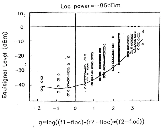
(3) Monte Carlo simulation is carried out for CDI evaluation. Since FM signal is a stochastic process, the spectrum mentioned here refers to the ensemble average of the Fourier transform of waveform in time domain, i.e. average spectrum. The IM spectrum in real radio environment differs from that in experimental condition. In real environment IM interference is the product of three FM signals, therefore the shape of its spectrum is the convolution of three FM spectra. In B1 immunity experiments one FM channels along with two pure carriers are served as input noises, so the shape of IM spectrum is the same as FM spectrum. Because the reproduction of experimental results is the pre-requisite to the theoretical works proposed here, the latter condition is adapted in our model. International Telecommunication Union (ITU) has defined the average power spectrum of an FM channel used in interference immunity experiments on ILS localizer receivers [20](see Figure 2.8a). The FM spectrum in Figure 2.8a has the 20-dB bandwidth 34 KHz. The power of frequency components outside the bandwidth is at most 0.01 times of that at center frequency. For simplicity we could assume that their contribution is negligible. In this thesis the shape of ITU FM power spectrum SFM(f) is approximated as a triangle within bandwidth BW and vanishes out of bandwidth, as in Figure 2.8b. The absolute value of average FM spectrum HFM(f) equals to V/SFM(f). Based on average FM

power spectrum Monte Carlo simulation on baseband model is possible. The ensemble

average and standard deviation of CDI values are functions of total interfering power

2.4 Modeling of Baseband Stage

(4) Baseband stage model should confirm to the ILS localizer receiver standards when there is no interference. First, CDI current is proportional to DDM (= m90 - m1_{5 0} ). If DDM= d corresponds to CDI= cIL A, then DDM= -d corresponds to CDI= -cpL A. Second, at full deflection DDM=0.155 corresponds to CDI current 150/LA. Before feeding into noise baseband stage model should be calibrated accordingly.

We use the following procedure to estimate CDI mean and standard deviation:

1. Calibrate the parameters of baseband stage model under signal-only conditions. The conditions needed to be satisfied are that (1) the simulated CDI equal to 150 p•A when DDM=0.155; (2) if the simulated CDI value is cI A when DDM value is

d, then the simulated CDI value will be -cIp A when DDM value becomes -d. 90

Hz filter gain and bandwidth, 150 Hz filter gain and bandwidth, and comparator gain are adjusted accordingly.

2. Choose the appropriate DDM value such that the simulated CDI=90 p A under signal-only conditions. This is the standard condition under which localizer receiver bench experiments were conducted. For a realistic receiver this DDM value is about 0.093.

3. Pick up a value for the average intermodulation interference power level. Generate a random interference spectrum by using the given average power level and the average power spectrum prescribed in Figure 2.8b.

4. Convert the intermodulation interference from frequency domain to time domain. Incorporate with the localizer component at IF output, Alo[1 + mgg cos(290 90t) +

Tm1 50 cos(27r- 150t)] cos(27rflFt) . Use the resultant temporal signal as baseband input to do the baseband-stage simulation.

5. Carry out different realizations from 3. to 4. Calculate the average and standard (deviatioin _{of CII values and other necessary statistical quantities.}

Chapter 2 Generic Model for ILS Receiver

6. Pick up different values for average interference power level, repeat 3. to 5. Construct the relationship of CDI mean and standard deviation to interference power level.

2.4.3 Modeling of Envelope Detector

The operation of an envelope detector could be obtained from circuit analysis. The structure of an envelope detector is a full-wave rectifier followed by a low-pass filter. Usually a four-diode bridge is served as rectifier, and a parallel RC circuit is served as low-pass filter. Figure 2.9 illustrates its circuit diagram.

out

Fig2.9 Envelope detector circuit

Assume D1, D2, D3, D4 are idea diodes. Only ON and OFF states apply to those diodes. For the ON state, the forward diode voltage Vd = 0 if the forward d(iolde current Id > 0; for the OFF state the diode current Id = 0 if the diode voltage Vd < 0 . Then the output is switched between two conditions: when D1/D3 or I)2/I)4 are ON, the output voltage follows the input voltage; when all diodes are OFF, the output voltage decays exlponentially with RC time constant. And the swit.chmiig is determined by the polarity of current. It is formulated as follows.

2.4 Modeling of Baseband Stage

vVuit(t0111() )cxp(0

VOI~

{

Ivin(Ol)I,

if _{if vo} vout(t) _{+ •Vout >} > Ivin(t)l ₀

The output could be approximated by discretizing continuous time into a series of finite steps:

tn = nAt

t V(( out(tn-1) exp( -), if vout(tn) > Ivin(tn)l

f(vout (tn) -Vout (tn-))

+

E vo u t (t n ) > 0

(2.4.5)

2.4.4 Modeling of Final Signal Processing Stage

As indicated in Figure 2.1, the detector output is fed into the 90 Hz and 150 Hz detection blocks simultaneously to retrieve the amplitudes of 90 Hz and 150 Hz components. The output signals from these two blocks are fed into a differential amplifier, hereby generates CDI current. The 90 Hz/150 Hz detection block contains a bandpass filter with central frequency 90/150 Hz and an envelope detector. The envelope detector has been modeled in Section 2.4.3. The bandpass filter is typically designed as a fourth-order Butterworth filter [26]:

IHbase(f)l

=

1I+i

f2

)

4

wllere f(.(lt?.,rl is its central frequllency, and 1311' is its bandwidth.

(2.4.4)

Chapter 2 Generic Model for ILS Receiver

Similar to Section 2.4.3, all the signal flow is simulated in discrete level. The simulation processes are arranged in this way:

1. Convert the discrete-time input signal (see (2.4.5)) into frequency-domain signal.

2. Multiply it with 90 Hz bandpass filter response Hbase(f) (see eqno(2.4.6)).

3. Inverse transform the resultant frequency-domain signal into time domain.

4. Pass through the envelope detector. Use (2.4.5) to evaluate the output.

5. Repeat (2) to (4) for 150 Hz portion.

6. Pass the results obtained from (4) and (5) into a differential amplifier to obtain the difference. Multiply it by a constant gain. Take time average of the result to get CDI output.

2.4.5 Approximation Scheme of IF Envelope Detector

The input of IF envelope detector (denoted by i,,(t)) contains IF localizer

signal and IF noise (denoted by N fM(t) ) with the specific average power spectrum (as indicated in Figure 2.10),

2.4 Modeling of Baseband Stage

The function of envelope detector model is to simulate the output temporal signal

zout(t) in response to the input xin (t). As described in Section 2.4.3, the operation of

an envelope detector can be numerically simulated by using finite-difference method. The IF envelope detector receives IF localizer signal and noise and converts them into the baseband. In order to avoid under-sampling the sampling rate should be comparable to fIF (or even higher since the interference contains higher frequency components). For a fixed total simulation duration T, the number of time steps for a single realization is -. O(T - fIF). The total simulation duration T is related to the frequency resolution. It should be longer than one period of 90 Hz ( 0.011sec).

fIF is in the order of MHz. In sixth-order Chebyshev model it is 30.5 MHz. So the

number of time steps, if estimated practically, is about the order of 106. A lot of computation time should be spent on simulating envelope detector.

An approximation scheme can be used to reduce computational complexity of direct simulation on envelope detector. The rationality of this scheme is that by replacing the original IF interference with a baseband interference at input, we can get approximately the same output. And the computational complexity of envelope detector simulation in response to this new input is much lower since the input has a

much smaller bandwidth. The method is depicted as follows.

Define a baseband noise Nbase(t) such that

NIMF(t) = NIM (t) -2 _cos(27rfIFt)

The Fourier transform of a time-domain signal x(t) is denoted by xF(f). It is obvious that the spectrum of baseband noise Nbse is a direct translation of IF noise spectrum.

IF f) bas ase (2.F

NIMIF(= NIAt F( f - f( F) + NI ! F(f + fIF) • (2.7) Now define a new inllut x*:r(t) to the samIie envClopC detector. It. contaills l)asc)ill(ld localizer signal and btaselani noise,