HAL Id: hal-00269407
https://hal.archives-ouvertes.fr/hal-00269407
Submitted on 18 Jul 2020
HAL is a multi-disciplinary open access
archive for the deposit and dissemination of
sci-entific research documents, whether they are
pub-lished or not. The documents may come from
teaching and research institutions in France or
abroad, or from public or private research centers.
L’archive ouverte pluridisciplinaire HAL, est
destinée au dépôt et à la diffusion de documents
scientifiques de niveau recherche, publiés ou non,
émanant des établissements d’enseignement et de
recherche français ou étrangers, des laboratoires
publics ou privés.
Solar and Heliospheric Observatory/solar Wind
Anisotropies Observations of five moderately bright
comets: 1999-2002
Michael R. Combi, J. Teemu T. Mäkinen, N.J. Henry, Jean-Loup Bertaux,
Eric Quémerais
To cite this version:
Michael R. Combi, J. Teemu T. Mäkinen, N.J. Henry, Jean-Loup Bertaux, Eric Quémerais.
So-lar and Heliospheric Observatory/soSo-lar Wind Anisotropies Observations of five moderately bright
comets: 1999-2002. Astronomical Journal, American Astronomical Society, 2008, 135 (4),
pp.1533-1550. �10.1088/0004-6256/135/4/1533�. �hal-00269407�
SOLAR AND HELIOSPHERIC OBSERVATORY/SOLAR WIND ANISOTROPIES OBSERVATIONS OF FIVE MODERATELY BRIGHT COMETS: 1999–2002
M. R. Combi1, J. T. T. M ¨akinen2, N. J. Henry1, J.-L. Bertaux3, and E. Quem´erais3
1Department of Atmospheric, Oceanic and Space Sciences, University of Michigan, 2455 Hayward Street, Ann Arbor, MI 48109-2143, USA;[email protected] 2Finnish Meteorological Institute, Box 503, SF-00101 Helsinki, Finland
3Service d’A´eronomie du CNRS, Universit´e de Versailles Saint-Quentin, BP3, 91371 Verri`eres le Buisson Cedex, France Received 2007 November 28; accepted 2008 February 5; published 2008 March 12
ABSTRACT
Solar Wind Anisotropies (SWAN), the all-sky hydrogen Lyman-alpha camera, on the SOHO spacecraft makes routine all-sky images of the interplanetary neutral hydrogen around the Sun and thus monitors the effect of the variable solar wind on its distribution. SWAN has an ongoing campaign to make special observations of comets, both short- and long-period ones, in addition to making serendipitous observations of comets as part of the all-sky monitoring program. We report here on a study of the moderately active Oort cloud comets observed by SWAN during the period of 1999–2002: 1999 H1 Lee, 1999 T1 McNaught Hartley, 2000 WM1 LINEAR, 2001 A2 LINEAR, and 2002 C1 Ikeya Zhang (P153). SWAN is able to observe comets almost continuously over most of their visible apparitions and provide excellent temporal coverage of water production. In addition to calculating production rates from each single image, we also present results using our time-resolved model (TRM) that analyzes an entire sequence of images over many days to several weeks/months, and from which daily-averaged or two-day-averaged water production rates are extracted over continuous periods of several days to months. The short-term (outburst) behavior is correlated with other observations and is examined and associated with fragment release. The long-term heliocentric distance-dependent variations of water production rate are examined and compared and contrasted with the measured volatile compositions of the comets as well as their absolute production rate levels. The overall long-term variation is also distinguished from seasonal effects seen in the pre- to post-perihelion differences.
Key words: comets: general – comets: individual (1999 H1 Lee, 1999 T1 McNaught-Hartley, 2001 A2 LINEAR,
2001 WM1 LINEAR, P153/Ikeya-Zhang) – molecular processes
1. INTRODUCTION
Observations of hydrogen Lyman-α (Ly-α) at 1215.7 Å in comets and their interpretation are important. Atomic hydrogen is the most abundant species in the atmosphere (or coma) of a comet being produced in a photodissociation chain originating with water molecules and including intermediate OH radicals. Water is the most abundant volatile species in a comet’s nucleus, and water sublimation controls the abundance and activity of the coma when comets are within 3 AU from the Sun. Measurements of the abundance and distribution of hydrogen in the coma, when appropriately modeled, can provide a reliable measure of the water production rate and its variation in time in comets. Virtually all compositional information is compared to water, making water the most important species for obtaining accurate production rates. Variations in production rate with time generally, and with heliocentric distance in particular can provide information about the composition and structure of the nucleus.
Solar Wind Anisotropies (SWAN), the all-sky hydrogen Ly-α camera, has been operating on the Solar and Heliospheric
Observatory (SOHO) spacecraft since its launch in 1995. The
SWAN instrument was designed to observe the entire sky in H Ly-α in order to obtain a global view of the variable interaction of the solar wind with the neutral interstellar hydrogen streaming through the solar system. From its viewpoint at the L1 Lagrange point between the Earth and Sun it obtains an unparallel view of the Sun, its large extended corona, and the entire sky. For a more detailed description of SWAN, see Bertaux et al. (1995).
Because of the limited observing time available for synoptic cometary observations (or any solar system targets for that
matter) with the Hubble Space Telescope (HST), compounded by the fact that many bright comets are often within the solar avoidance area of the HST, space-based observations, and in particular ultraviolet (UV) observations, have been severely limited in recent years compared with most of the previous 20 years when IUE was available. SWAN with its UV capability has filled an important void in the monitoring of comets from space since early 1996.
Because of the large neutral hydrogen coma, SWAN can observe comets either in the nominal full-sky mode, when comets are recorded during the nominal full-sky interplanetary medium observations, or during special campaigns of comet-specific observations, when the region of the sky with a comet is specifically targeted and sometimes oversampled by the SWAN instrument field of view (IFOV) to yield a somewhat improved spatial resolution. We report here on a set of moderately bright comets observed by SWAN during the period of 1999–2004, which includes 1999 H1 Lee, 1999 T1 McNaught Hartley, 2000 WM1 LINEAR, 2001 A2 LINEAR, and 2002 C1 Ikeya Zhang (P153). The single-image water production rates are presented. We also used our time-resolved model (TRM) to analyze long sequences of images simultaneously to obtain deconvolved daily-average or two-day-average water production rates between the image snapshots. Because we are presenting results from several comets, the paper is organized such that we discuss comet observations generally, followed by a discussion of the model analysis procedure, and then followed by a discussion of each comet. In each of these sections, we examine the variation of the water production rates with time and heliocentric distance, discuss their significance, and compare with other observations. The paper concludes with a general summary.
2. OBSERVATIONS
The observations presented in this paper result from two basic observational modes. SWAN routinely observes the full sky two to three times per week. Any comet bright enough will be registered on full-sky images. When a bright or otherwise interesting comet is expected, comet-specific observations are also planned and made. The comet-specific images can improve the spatial resolution by oversampling and reduce the noise by longer integrations over the full-sky images (M¨akinen & Combi 2005). For the previous results on comet 1996 B2 (Hyakutake) the comet-specific images were more important when the comet was very close to the Earth because of its large proper motion during the time the full-sky images are acquired. In that case Combi et al. (2005) accounted for any motion issues in the daily-averaged deconvolution with the TRM. These effects are included in the formal uncertainties in the single-image production rates and as well in the daily-averaged deconvolved results given in the next section. Tables giving the observational circumstances for all the SWAN images for each comet as well as the single-image production rates are presented below in the sections on each comet. The g-factor was derived from daily-average observations by the SOLSTICE instrument on UARS, which measures the solar UV irradiance. It is corrected to first order for the solar radiation difference between the face of the Sun seen by SOHO and that seen by the comet (Combi et al. 2000) and for the Doppler shift of the Ly-α line profile caused by the heliocentric radial velocity of the comet.
3. TIME-RESOLVED MODEL
We have used the TRM to extract the time history of the water production rate by analyzing the various series of images together. The details of the model are described in the paper by M¨akinen & Combi (2005). Because of its long lifetime (∼1.5 × 10⁶s at 1 AU from the Sun), H atoms survive in the coma for 2–4
weeks, during which time there are often available up to five to ten SWAN images of the coma. The TRM uses a parametrized velocity distribution for H atoms in the coma, estimated from explicit calculations of the partial thermalization by the heavy-atom coma (Combi & Smyth1988a,1988b; Combi et al.2000), and tracks their propagation out into the coma. The method then builds up a set of basis functions relating the production rate of water at the nucleus as a function of time to the distribution of photodissociated H atoms as seen on the sky plane. In this paper, we present results of the water production rates in the standard single-image form as well as daily-averaged and two-day-averaged deconvolved water production rates extracted by the inversion scheme of the TRM.
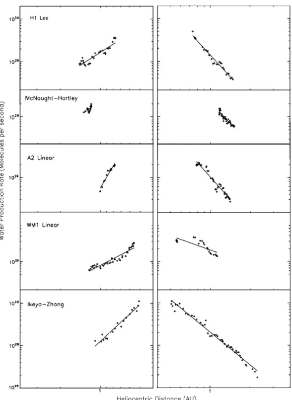
4. 1999 H1 LEE
Comet 1999 H1 Lee (hereafter also referred to as Lee) is a long-period Oort cloud comet that reached a perihelion distance of 0.708 AU on 1999 July 11.1772 UT. Observations of the com-position of Lee generally found abundances of most volatiles to be comparable to Oort cloud comets, except for CO, which was only present at the 2–4% level (Biver et al.2000; Mumma et al. 2001b). SWAN observations show the H coma of comet Lee from 1999 April 10 to September 20 covering a heliocentric dis-tance range from 1.43 AU before perihelion to 1.48 after. Table 1gives the observational circumstances and single-image water production rates determined using the TRM. In this mode an entire image is analyzed, assuming a nominal time/heliocentric
distance variation (r−2), and a single production rate is deter-mined for the time of the observation using the entire image. The top panel of Figure1shows the pre- and post-perihelion production rates plotted as a function of heliocentric distance. Past experience shows that the long-term heliocentric distance dependence, usually fitted as a variation in the usual r−pform, is well represented in this way, as are general pre- to post- perihe-lion variation asymmetries. The daily-averaged deconvolution is most suited to fill in gaps between images and for correct time phasing of transient short-term activity variations. The power-law fits are shown as straight lines in the top set of panels in Figure1. The power-law fits for comet Lee are given in the top line of Table2for the pre- and post-perihelion legs as well as the averaged pre- and post-perihelion values.
Chiu et al. (2001) observed Lee with the Submillimeter Wave Astronomy Satellite (SWAS) and determined water production rates over the range of heliocentric distances from 1.3 to 1.7 AU after perihelion. Over this range they reported a value of 1.45× 1029s−1at 1 AU and an exponent of−5.5. The SWAN
observations on the other hand cover both legs but not as far out as 1.7 AU. Neufeld et al. (2000), on the other hand, presented a single water production rate from SWAS observations before perihelion on May 19–23.
Biver et al. (2000) reported on radio observations of various species in Lee with a number of radio telescopes. From obser-vations of OH and assuming that the water production rate was 1.1 times the OH production rate they report a power law of 8.0 × 1028r−2.3water molecules s−1. Their firm results are limited
to the pre-perihelion leg with a range of heliocentric distances from 1.36 to 0.93 AU. For the post-perihelion period when they had no good OH observations they monitored the gas production variation with heliocentric distance by following the production rate of HCN, which they find is about 1/900 of the water pro-duction rate. After perihelion they find that the gas propro-duction rate variation is steeper with an exponent closer to−3, and in general agreement with the pre- to post-perihelion asymmetry we find. They also report that post-perihelion production rates are about 30% lower than pre-perihelion, where we find a ratio of the 1 AU values of about 121%—however, the exact value of the ratio depends in part on the specific heliocentric distances covered and ratioed.
Other water production rates covering limited ranges of heliocentric distance have been reported by Weaver et al. (2002), Mumma et al. (2001b), Neufeld et al. (2000), Feldman et al. (1999), Lara et al. (2004a), and Dello Russo et al. (2005). These, as well as those discussed above from Chiu et al. and Biver et al., are plotted in Figure2along with the TRM daily-averaged deconvolved water production rates from SWAN, which are given in Table 3. The values from Biver et al. show the same temporal variation but are about 25% below SWAN. The values of Chiu et al., as mentioned, are mostly at larger post-perihelion heliocentric distances, but are about half of the SWAN values in the overlap region. The values of Dello Russo et al., Mumma et al., Feldman et al., and Neufeld et al. are comparable with some a little larger and some a little smaller. The preliminary value of Weaver et al. (1999), as reported in Biver et al. (2000), from ground-based IR observations seems anomalously low compared with all other observations including IR observations by Dello Russo et al. and Mumma et al. Taken together, and acknowledging the usual systematic differences between different observed species and model parameters, there is general consistency in describing the higher pre-perihelion level and the steeper fall-off
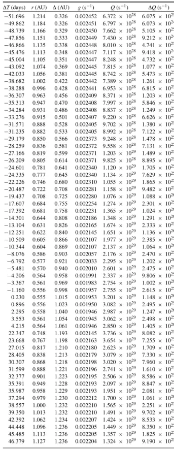
Table 1
Comet Lee: Observational Circumstances and Single-Image Water Production Rates
∆T (days) r (AU) ∆ (AU) g (s−1) Q (s−1) ∆Q (s−1)
−66.544 1.434 0.722 0.002248 8.854× 1028 1.171× 1025 −65.374 1.417 0.723 0.002249 9.148× 1028 6.154× 1025 −63.979 1.397 0.727 0.002251 8.728× 1028 1.151× 1025 −63.472 1.389 0.729 0.002251 1.039× 1029 4.901× 1025 −61.516 1.361 0.740 0.002252 1.240× 1029 1.415× 1025 −60.468 1.346 0.748 0.002226 1.059× 1029 5.051× 1025 −59.502 1.332 0.757 0.002227 9.492× 1028 1.150× 1025 −58.412 1.316 0.767 0.002228 8.537× 1028 6.512× 1025 −56.504 1.289 0.789 0.002230 8.103× 1028 7.264× 1025 −52.316 1.229 0.848 0.002233 8.655× 1028 7.266× 1025 −50.724 1.206 0.874 0.002235 9.029× 1028 6.855× 1025 −49.660 1.191 0.892 0.002236 9.138× 1028 8.167× 1025 −46.665 1.149 0.946 0.002239 1.320× 1029 6.569× 1025 −44.606 1.120 0.985 0.002240 1.219× 1029 7.751× 1025 −42.679 1.093 1.022 0.002215 1.582× 1029 6.832× 1025 −37.608 1.024 1.123 0.002219 1.655× 1029 7.534× 1025 −35.692 0.999 1.161 0.002197 1.770× 1029 6.309× 1025 −32.695 0.960 1.221 0.002200 1.855× 1029 6.770× 1025 −30.637 0.934 1.261 0.002179 1.587× 1029 7.821× 1025 −28.991 0.914 1.293 0.002158 1.615× 1029 1.815× 1025 −28.709 0.911 1.298 0.002158 1.531× 1029 8.698× 1025 −25.380 0.872 1.360 0.002141 2.039× 1029 6.497× 1025 −22.994 0.846 1.403 0.002123 2.110× 1029 6.306× 1025 −19.175 0.807 1.467 0.002089 2.941× 1029 5.294× 1025 −16.905 0.786 1.502 0.002056 3.616× 1029 5.140× 1025 −14.648 0.768 1.535 0.002042 3.550× 1029 5.965× 1025 10.193 0.738 1.682 0.001953 4.977× 1029 2.377× 1025 14.101 0.764 1.666 0.001993 3.558× 1029 9.490× 1025 15.771 0.777 1.657 0.002005 3.380× 1029 1.705× 1025 25.544 0.874 1.569 0.002080 2.168× 1029 7.775× 1025 27.479 0.896 1.546 0.002096 1.842× 1029 7.330× 1025 30.493 0.932 1.507 0.002116 1.805× 1029 7.095× 1025 32.563 0.958 1.479 0.002117 1.749× 1029 7.274× 1025 34.516 0.983 1.451 0.002136 1.375× 1029 8.404× 1025 37.529 1.023 1.405 0.002156 1.120× 1029 8.214× 1025 39.599 1.051 1.373 0.002158 8.701× 1028 9.015× 1025 41.537 1.077 1.342 0.002159 9.014× 1028 8.464× 1025 44.551 1.119 1.292 0.002181 8.433× 1028 8.805× 1025 46.621 1.148 1.257 0.002182 8.324× 1028 9.218× 1025 48.571 1.176 1.223 0.002184 9.669× 1028 7.807× 1025 50.126 1.198 1.197 0.002185 9.035× 1028 1.554× 1025 51.570 1.218 1.172 0.002186 8.852× 1028 7.435× 1025 53.639 1.248 1.137 0.002187 6.985× 1028 8.800× 1025 55.435 1.273 1.107 0.002189 6.484× 1028 8.996× 1025 58.884 1.323 1.050 0.002191 4.787× 1028 1.086× 1026 60.775 1.350 1.020 0.002192 5.152× 1028 1.048× 1026 62.698 1.378 0.991 0.002213 5.098× 1028 1.133× 1026 65.740 1.422 0.948 0.002215 3.883× 1028 1.185× 1026 67.998 1.455 0.919 0.002217 4.078× 1028 1.026× 1026 69.933 1.483 0.897 0.002199 3.719× 1028 1.099× 1026 Notes.
∆T: time from perihelion 1999 July 11, in days for each SWAN image.
r: heliocentric distance (AU).
∆: geocentric distance (AU).
g: solar Lyman-α g-factor (photons s−1).
Q: water production rates for each image (s−1). ∆Q: 1σ formal uncertainty (s−1).
post-perihelion. The SWAS observations indicate that the gas production rate has a fairly steep fall-off for distance larger than 1.5 AU. Comet Lee is low in CO (Biver et al.2000; Mumma et al.2001b) while its CH3OH abundance is enhanced and ethane
and acetylene are similar to volatile-rich bright comets such as
Hyakutake and Hale–Bopp. The post-perihelion drop could be indicative of a simple seasonal effect of the nucleus rotation axis exposing different portions of the nucleus surface. It is noteworthy that Biver et al. report CO depletion pre-perihelion and Mumma et al. report CO depletion post-perihelion, so it does
Figure 1. Single-image water production rates and fitted power-law distributions.
not appear that there is a gross change in chemical composition before and after perihelion that would be indicative of gross chemical heterogeneity around the surface.
In the overall SWAN light curve of daily-averaged production rates, there appear to be a few transient features, with small outbursts on the order of 20–40% increases in gas production rate lasting several days each at −67 days, −46 days, +2 days, and +47 days measured from perihelion. Such variations determined from SWAN observations were corroborated in the
case of comet Hyakutake (Bertaux et al.1998; Combi et al. 2005) which was observed more intensely by many groups than was Lee.
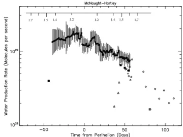
5. 1999 T1 McNAUGHT-HARTLEY
Comet 1999 T1 McNaught-Hartley (hereafter also referred to as M-H) reached a perihelion distance of 1.1717 AU on 13.4722 December (UT), 2000. SWAN observations of
McNaught-Table 2
Power-Law Fits to the Water Production Rate Variation
Comet Q1 P Q1(pre) P (pre) Q1(post) P (post)
1999 H1 Lee 1.5 × 1029 −2.7 1.7× 1029 −2.0 ± 0.2 1.4× 1029 −3.4 ± 0.1 1999 T1 McNaught-Hartley 2.9 × 1029 −3.3a 2.4× 1029 −2.4 ± 0.7 2.2× 1029 −3.3 ± 0.2 C 2001 A2 LINEAR 9.3 × 1028 −4.5 5.6× 1028 −5.3 ± 0.4 1.1× 1029 −3.7 ± 0.1 C 2001 WM1 LINEAR 1.1 × 1029 −1.4 8.2× 1028 −1.6 ± 0.1 1.8× 1029 −1.1 ± 0.2 P153/Ikeya-Zhang 1.8 × 1029 −2.7 1.2× 1029 −2.9 ± 0.2 2.0× 1029 −2.6 ± 0.1 C 1995 OI Hale–Bopp 1.3 × 1031 −2.6 C 1996 B2 Hyakutake 2.7 × 1029 −2.1 Notes.
aBecause of the limited range of heliocentric distance in the data pre-perihelion we have adopted the post-perihelion slope for the
“average.”
Q1: water production rate at 1 AU: pre and post signify pre-perihelion and post-perihelion. P: power-law exponent in rp: pre and post signify pre-perihelion and post-perihelion.
0.8 1.0 1.2
1.4 0.8 1.0 1.2 1.4
1.6 1.6
Figure 2. Daily-average water production rates of comet 1999 H1 (Lee). The
SWAN results are plotted as small diamonds with vertical lines corresponding to one-sigma uncertainties. The other water production rate values are: left pointing triangles, Biver et al. (2000); right pointing triangle, Lara et al. (2004a); +, Chiu et al. (2001); open square, Weaver et al. (2002); filled square, Feldman et al. (1999);×, Mumma et al. (2001b) and Dello Russo et al. (2005). The inset scale gives the heliocentric distance in AU.
Hartley are available from early 2000 November to 2001 mid-February. Because of its larger perihelion distance the total length of time when its brightness in Ly-α was high enough to extract good water production rates was limited com-pared with the other comets in this group. The combination of large heliocentric distance and large production rate made the detectability of M-H similar to the other comets in this group at the beginning and end of the run of useful images. The observational circumstances of the individual SWAN im-ages and the single-image water production rates are given in Table4.
The second panel of Figure1shows the results of the single-image water production rates for McNaught-Hartley plotted as a function of heliocentric distance. Because of the limited heliocentric distance range, especially before perihelion, it is not clear how much significance to place in the power-law exponent before perihelion. The post-perihelion slope is−3.3. Because of the limited range of heliocentric distances in the pre-perihelion data, we adopted the post-perihelion slope as the “average” value for this comet. The production rate projected back to 1 AU— note that the comet only gets to 1.17 AU—is∼2.3 × 1029s−1,
1.2
1.4 1.2 1.4
1.7 1.5 1.5 1.7
Figure 3. Daily-averaged water production rates of comet 1999 T1
(McNaught-Hartley). See Figure2caption for details. The other water production rate values are: filled square, Biver et al. (2006); isolated diamonds, Bensch et al. (2004); open square, Weaver et al. (2002); +, Vervack et al. (2004); upward-pointing triangle, Lovell et al. (2008). The inset scale gives the heliocentric distance in AU.
and so while this was not a particularly spectacular object, its gas production rate, if it were at smaller heliocentric distances, is comparable to the more active comets in the group presented here.
Figure3and Table5give the daily-average water production rates extracted from the whole set of SWAN images as a function of time from perihelion plotted with a number of other measurements yielding water production rates. Again the SWAN values are slightly higher but reasonably consistent with observations by SWAS (Bensch et al.2004) who observed after perihelion. The post-perihelion radio OH observations by Biver et al. (2006) are consistent with both SWAS (and SWAN) but the single pre-perihelion measurement 43 days before perihelion is a factor of 3 below the SWAN value. There are other single measurements by Vervack et al. (2004) and Weaver et al. (2002), which are consistent with SWAS and Biver et al. Several values from radio OH measurements by Lovell et al. (2008) are a factors of 3–5 below the SWAN values, far below the more typical difference of 25% between SWAN and SWAS or the Biver et al. radio measurements. The other water production rates (mostly from SWAS) extend the SWAN activity light curve out to just past 2 AU after perihelion and indicate that the steep fall-off
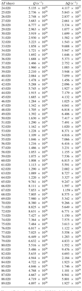
Table 3
Comet Lee: Deconvolved Daily-Averaged Water Production Rates
∆T (days) Q (s−1) ∆Q (s−1) −78.173 6.633× 1028 2.946× 1028 −77.173 6.746× 1028 2.609× 1028 −76.173 6.905× 1028 2.607× 1028 −75.173 7.002× 1028 2.058× 1028 −74.173 6.547× 1028 1.319× 1028 −73.173 6.223× 1028 8.458× 1027 −72.173 6.588× 1028 8.765× 1027 −71.173 6.984× 1028 8.657× 1027 −70.173 7.413× 1028 7.613× 1027 −69.173 7.357× 1028 6.849× 1027 −68.173 7.183× 1028 5.934× 1027 −67.173 9.443× 1028 6.688× 1027 −66.173 1.368× 1029 1.683× 1028 −65.173 1.008× 1029 1.466× 1028 −64.173 9.165× 1028 1.101× 1028 −63.173 8.675× 1028 8.351× 1027 −62.173 8.485× 1028 9.305× 1027 −61.173 8.382× 1028 1.045× 1028 −60.173 8.254× 1028 1.882× 1028 −59.173 8.634× 1028 1.882× 1028 −58.173 8.031× 1028 1.990× 1028 −57.173 8.118× 1028 1.825× 1028 −56.173 8.269× 1028 1.569× 1028 −55.173 8.803× 1028 1.209× 1028 −54.173 1.007× 1029 7.047× 1027 −53.173 9.925× 1028 1.371× 1028 −52.173 1.036× 1029 1.626× 1028 −51.173 1.097× 1029 2.342× 1028 −50.173 1.153× 1029 2.312× 1028 −49.173 1.244× 1029 2.282× 1028 −48.173 1.212× 1029 2.011× 1028 −47.173 1.306× 1029 1.904× 1028 −46.173 1.481× 1029 2.310× 1028 −45.173 1.702× 1029 2.387× 1028 −44.173 1.240× 1029 4.508× 1028 −43.173 1.281× 1029 4.358× 1028 −42.173 1.300× 1029 3.718× 1028 −41.173 1.383× 1029 4.456× 1028 −40.173 1.410× 1029 3.566× 1028 −39.173 1.448× 1029 4.179× 1028 −38.173 1.487× 1029 3.357× 1028 −37.173 1.415× 1029 5.051× 1028 −36.173 1.414× 1029 4.090× 1028 −35.173 1.415× 1029 4.176× 1028 −34.173 1.368× 1029 3.144× 1028 −33.173 1.538× 1029 4.246× 1028 −32.173 1.526× 1029 3.118× 1028 −31.173 1.692× 1029 6.506× 1028 −30.173 1.686× 1029 5.056× 1028 −29.173 1.969× 1029 7.495× 1028 −28.173 2.084× 1029 5.333× 1028 −27.173 1.960× 1029 5.546× 1028 −26.173 1.993× 1029 4.595× 1028 −25.173 2.215× 1029 5.357× 1028 −24.173 2.249× 1029 4.423× 1028 −23.173 2.693× 1029 6.398× 1028 −22.173 2.828× 1029 5.058× 1028 −21.173 3.147× 1029 9.038× 1028 −20.173 3.240× 1029 7.550× 1028 −19.173 3.020× 1029 1.680× 1029 −18.173 3.102× 1029 1.254× 1029 −13.173 4.549× 1029 1.224× 1030 −12.173 4.088× 1029 1.031× 1030 −11.173 4.020× 1029 6.531× 1029 −10.173 4.069× 1029 6.453× 1029 Table 3 (Continued) ∆T (days) Q (s−1) ∆Q (s−1) −9.173 3.750× 1029 5.633 × 1029 −8.173 3.780× 1029 5.486 × 1029 −7.173 3.504× 1029 4.444 × 1029 −6.173 3.462× 1029 3.761 × 1029 −5.173 3.711× 1029 5.429 × 1029 −4.173 3.764× 1029 5.272 × 1029 −3.173 4.779× 1029 4.831 × 1029 −2.173 4.913× 1029 4.550 × 1029 −1.173 4.820× 1029 3.259 × 1029 −0.173 4.869× 1029 4.117 × 1029 0.827 7.397× 1029 4.721 × 1029 1.827 7.267× 1029 4.569 × 1029 2.827 3.852× 1029 7.974 × 1028 3.827 3.462× 1029 4.382 × 1028 4.827 4.337× 1029 1.280 × 1029 5.827 4.264× 1029 1.148 × 1029 6.827 3.896× 1029 8.525 × 1028 7.827 3.905× 1029 4.603 × 1028 8.827 2.745× 1029 4.152 × 1028 9.827 2.717× 1029 3.745 × 1028 10.827 2.645× 1029 1.994 × 1028 11.827 2.628× 1029 1.044 × 1028 12.827 3.384× 1029 1.894 × 1029 13.827 3.153× 1029 1.529 × 1029 14.827 2.900× 1029 1.345 × 1029 15.827 2.719× 1029 1.121 × 1029 16.827 2.483× 1029 1.077 × 1029 17.827 2.564× 1029 9.893 × 1028 18.827 2.378× 1029 9.951 × 1028 19.827 2.310× 1029 8.180 × 1028 20.827 2.231× 1029 7.804 × 1028 21.827 2.210× 1029 6.429 × 1028 22.827 2.242× 1029 7.776 × 1028 23.827 2.092× 1029 5.466 × 1028 24.827 1.955× 1029 7.520 × 1028 25.827 1.915× 1029 6.269 × 1028 26.827 1.862× 1029 6.573 × 1028 27.827 1.865× 1029 5.352 × 1028 28.827 1.713× 1029 6.151 × 1028 29.827 1.717× 1029 5.033 × 1028 30.827 1.463× 1029 4.857 × 1028 31.827 1.451× 1029 3.793 × 1028 32.827 1.234× 1029 3.711 × 1028 33.827 1.198× 1029 2.861 × 1028 34.827 1.140× 1029 3.645 × 1028 35.827 1.084× 1029 2.888 × 1028 36.827 1.086× 1029 3.377 × 1028 37.827 1.062× 1029 2.812 × 1028 38.827 1.012× 1029 3.161 × 1028 39.827 9.887× 1028 2.607 × 1028 40.827 9.629× 1028 2.180 × 1028 41.827 9.510× 1028 1.529 × 1028 42.827 9.606× 1028 2.238 × 1028 43.827 9.637× 1028 1.743 × 1028 44.827 1.017× 1029 2.543 × 1028 45.827 1.049× 1029 1.979 × 1028 46.827 1.038× 1029 3.300 × 1028 47.827 1.066× 1029 2.765 × 1028 48.827 8.011× 1028 3.233 × 1028 49.827 7.950× 1028 2.671 × 1028 50.827 7.449× 1028 2.880 × 1028 51.827 7.318× 1028 2.394 × 1028 52.827 6.678× 1028 2.405 × 1028 53.827 6.551× 1028 2.005 × 1028 54.827 6.216× 1028 1.622 × 1028
Table 3 (Continued) ∆T (days) Q (s−1) ∆Q (s−1) 55.827 6.015× 1028 1.308× 1028 56.827 6.037× 1028 1.228× 1028 57.827 6.167× 1028 9.691× 1027 58.827 5.682× 1028 1.265× 1028 59.827 5.699× 1028 1.038× 1028 60.827 4.893× 1028 1.382× 1028 61.827 4.861× 1028 1.224× 1028 62.827 4.930× 1028 1.071× 1028 63.827 4.639× 1028 1.401× 1028 64.827 4.665× 1028 1.247× 1028 65.827 4.896× 1028 1.013× 1028 Notes.
∆T: time from perihelion 1999 July 11, in days for each deconvolved value.
Q: water production rates for each image (s−1). ∆Q: 1σ formal uncertainty (s−1).
of production rate seen in the SWAN data continues to become even steeper at larger heliocentric distances.
Comet McNaught-Hartley was relatively CO rich. Biver et al. (2006) report a CO/H2O ratio of 15%, which is comparable to
the highest values like comet Hale–Bopp. Others of the principal minor species (CH3OH, H2CO, and HCN) are fairly nominal and
slightly underabundant compared with Hale–Bopp. What seems remarkable about McNaught-Hartley is the combination of high CO abundance with as steep fall-off of water production with heliocentric distance. The high CO production rate comets such as 1995 O1 Hale–Bopp and 1996 B2 Hyakutake have moderate slopes, in the range of−2. Usually, less productive short-period Jupiter family comets have steep slopes and are not usually know to have high CO abundances.
Finally, the daily-averaged water production rate values show some minor temporal structure, but only at the ∼20% level with increases (outbursts?) 10 days and 41 days after peri-helion. While the post-perihelion variation otherwise follows the monotonic long-term power law, the limited pre-perihelion shape seems to be dominated by some irregular structure, but not outbursts. Perhaps this is an indication of a seasonal change in the pole orientation during the pre-perihelion leg around 30 days before perihelion.
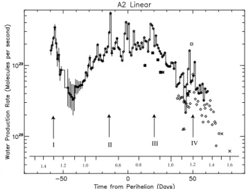
6. 2001 A2 LINEAR
Comet C/2001 A2 (LINEAR) (hereafter also referred to as A2) is noteworthy because of its spectacular splitting events (Jehin et al. 2002; Boehnhardt 2002; Sekanina et al. 2002; Furusho et al. 2003). It reached a perihelion distance of 0.779 AU on 24.5237 May (UT), 2001. SWAN observational results are available from 2001 late-March through the end of 2001 July covering heliocentric distances from 1.36 AU before perihelion to 1.41 AU after perihelion. Table6shows the observational circumstances and single-image water production rates using the TRM.
The third panel of Figure 1 shows the single-image water production rates for A2 plotted as a function of heliocentric dis-tance. The production rates were somewhat lower than the other comets in the group presented here, limiting the length of time coverage of the observations and the penultimate heliocentric distances. Also plotted are the straight lines corresponding to the power-law fits to the production rate variation with heliocentric
I II III IV
0.8 1.0 1.2
1.4 0.8 1.0 1.2 1.4 1.6
Figure 4. Daily-averaged water production rates of comet C/2001 A2
(LINEAR). See Figure 2caption for details. The other water production rate values are: isolated diamonds, Bensch et al. (2004); filled squares, Biver et al. (2006); upward-pointing triangles, Lovell et al. (2008); ×, Bonev/Mumma/Dello Russo; open square, Weaver et al. (2002). The inset scale gives the heliocentric distance in AU. The Roman numerals I through IV mark the outburst events noted by Sekanina et al. (2002).
distance. The values are given in the third row of Table2. As will be discussed below, the production rate variation is highly asymmetric about perihelion. For A2 we have calculated the pre-perihelion power law only for the data after the large out-burst around 55 days before perihelion dissipated. Otherwise the variation is nearly flat and does not represent the orderly vari-ation of gas production. Without the early outburst the power law is steeper before perihelion (−5.3) than after (−3.7) and the overall magnitude of gas production after perihelion (5.6× 1028 s−1 at 1 AU) is nearly a factor of 2 smaller than before
(1.1× 1029s−1at 1 AU). We will return to the discussion of
the overall activity level variation below in the context of the outbursts and splitting events.
In Figure4and Table7we present the daily-averaged pro-duction rates for A2, and they are compared with a number of water production rate results by other investigators. Nearly all of the other observations were during the post-perihelion period. SWAS (Bensch & Melnick 2006) observed C/2001 A2 (LINEAR) after perihelion beginning on 2001 June 29 when the comet was at a heliocentric distance of 1.035 AU and ending on 2001 August 2 when the comet was at 1.497 AU, extending a week past the last SWAN observation. The SWAS water production rates are about 50% below the SWAN values before the large outburst in early July after which the overlapping SWAN and SWAS values are consistent to within the scatter. The SWAS measurements then continue on the same trend line for times after the last SWAN ob-servation. These later SWAS values are consistent with the later measurements from infrared water observations (Dello Russo et al. 2005; Bonev et al. 2004), which themselves are consistent with the earlier SWAN measurements. Weaver et al. (2002) reported a water production rate from Far
Ultravi-olet Spectroscopic Explorer (FUSE) observations of H2, H, and
OI in A2 around the time of the large outburst 48 days after perihelion and that single value is a factor of 4 higher than all other values during the same time period. While it is possible that FUSE was seeing an especially enhanced column in its relatively smaller aperture right near the outburst, the TRM
de-Table 4
Comet McNaught-Hartley: Observational Circumstances and Single-Image Water Production Rates
∆T (days) r (AU) ∆ (AU) g (s−1) Q (s−1) ∆Q (s−1)
−40.428 1.333 1.910 0.002230 1.270× 1029 1.732× 1026 −35.475 1.298 1.884 0.002217 1.360× 1029 1.427× 1026 −29.101 1.259 1.847 0.002191 1.527× 1029 1.400× 1026 −27.714 1.251 1.838 0.002191 1.586× 1029 1.315× 1026 −26.651 1.245 1.832 0.002191 1.554× 1029 1.283× 1026 −24.377 1.234 1.816 0.002181 1.445× 1029 1.364× 1026 −22.895 1.226 1.806 0.002181 1.298× 1029 1.448× 1026 −20.534 1.216 1.790 0.002170 1.234× 1029 1.781× 1026 −18.411 1.207 1.774 0.002161 1.314× 1029 1.355× 1026 −15.929 1.199 1.755 0.002152 1.377× 1029 1.336× 1026 −11.905 1.187 1.723 0.002143 1.513× 1029 1.244× 1026 −10.836 1.184 1.714 0.002136 1.736× 1029 1.238× 1026 −9.502 1.181 1.703 0.002136 1.534× 1029 1.408× 1026 −7.114 1.177 1.682 0.002130 1.820× 1029 2.366× 1025 −5.643 1.175 1.670 0.002130 1.776× 1029 1.251× 1026 −3.751 1.173 1.653 0.002124 1.821× 1029 9.894× 1025 −3.132 1.173 1.647 0.002124 2.002× 1029 2.098× 1025 −0.399 1.172 1.623 0.002121 1.708× 1029 1.059× 1026 0.201 1.172 1.617 0.002121 1.551× 1029 2.581× 1025 1.650 1.172 1.604 0.002120 1.108× 1029 1.837× 1026 5.201 1.175 1.571 0.002117 1.157× 1029 3.205× 1025 6.596 1.176 1.558 0.002115 1.266× 1029 1.393× 1026 8.665 1.180 1.539 0.002114 1.424× 1029 1.404× 1026 9.761 1.182 1.529 0.002114 1.391× 1029 2.714× 1025 10.581 1.184 1.521 0.002114 1.421× 1029 1.046× 1026 13.610 1.191 1.493 0.002112 1.525× 1029 1.187× 1026 15.679 1.198 1.475 0.002113 1.398× 1029 1.203× 1026 20.625 1.216 1.432 0.002116 1.038× 1029 1.490× 1026 22.368 1.224 1.417 0.002116 1.141× 1029 1.441× 1026 27.577 1.250 1.377 0.002124 9.930× 1028 1.323× 1026 28.082 1.253 1.373 0.002124 9.054× 1028 2.707× 1025 29.522 1.261 1.363 0.002124 7.964× 1028 1.408× 1026 31.634 1.274 1.350 0.002132 9.308× 1028 1.213× 1026 35.057 1.295 1.330 0.002141 9.918× 1028 1.154× 1026 36.112 1.302 1.324 0.002141 8.994× 1028 1.144× 1026 37.397 1.311 1.318 0.002141 8.829× 1028 2.531× 1025 38.190 1.317 1.314 0.002150 8.950× 1028 1.202× 1026 39.257 1.324 1.310 0.002150 7.947× 1028 1.252× 1026 40.955 1.337 1.303 0.002150 6.990× 1028 1.619× 1026 43.022 1.352 1.297 0.002162 7.118× 1028 1.502× 1026 44.277 1.362 1.293 0.002162 7.364× 1028 2.621× 1025 45.095 1.368 1.291 0.002162 8.859× 1028 1.191× 1026 47.842 1.390 1.287 0.002174 7.733× 1028 1.242× 1026 49.915 1.407 1.285 0.002173 8.115× 1028 1.110× 1026 51.124 1.418 1.285 0.002173 7.546× 1028 2.859× 1025 51.983 1.425 1.285 0.002173 6.838× 1028 1.210× 1026 53.038 1.434 1.286 0.002186 6.135× 1028 1.427× 1026 54.735 1.449 1.288 0.002186 6.372× 1028 1.339× 1026 56.803 1.467 1.292 0.002185 6.351× 1028 1.333× 1026 57.854 1.477 1.294 0.002185 6.351× 1028 1.303× 1026 59.755 1.494 1.300 0.002199 6.252× 1028 1.277× 1026 62.792 1.523 1.312 0.002198 6.128× 1028 1.336× 1026 Notes.
∆T: time from perihelion 2000 December 13, in days for each SWAN image.
r: heliocentric distance (AU).
∆: geocentric distance (AU).
g: solar Lyman-α g-factor (photons s−1).
Q: water production rates for each image (s−1). ∆Q: 1σ formal uncertainty (s−1).
convolution of the water production at the nucleus shows some more structure in the variation within a day before the FUSE measurement and another just after the maximum value
reg-istered by SWAS. Radio measurements of OH by Biver et al. (2006) are in good agreement with the SWAN results except for one radio measurement 10 days after perihelion that is a factor
of 2 below the SWAN results. The radio OH measurements by Lovell et al. (2008) at 41 days after perihelion are a factor of 3 or more below both SWAN and the other measurements.
Sekanina et al. (2002) have made a careful study of images of released fragments of A2 as well as associated outbursts of activity seen in its visual magnitude record. Our nearly continuous run of daily-averaged water production rates from SWAN provide yet a different comparison, where the TRM deconvolution process potentially places the initial timing of the outburst better than its response as seen in a global visual magnitude estimate. The large outbursts marked number I through IV by Sekanina et al. are all clearly seen in the SWAN results and the outburst IV was also seen in the SWAS results. Both the visual light curve of Sekanina et al. and SWAS measurements delineate an outburst at time 50–51 days after perihelion and is between two peaks recorded in the daily-averaged deconvolution of the SWAN data, with the second peak somewhat closer to the light curve/SWAS peak. The first of the two peaks is seen at 47.5 days after perihelion. The first peak is very close to the one large value from the HST (Weaver et al.2002) that probably not coincidentally was taken with a very small aperture, which naturally decreases the time smear and time lag. Extra irregular features were seen in synthetic image deconvolution testing shown in the model (M¨akinen & Combi2005) using a Hyakutake-like outburst which was about as large as this one and when field stars and longer and irregular time gaps between images were present in the input dataset.
An interesting comparison with the visual light curve (Sekanina et al. 2002) can also be made with the SWAN re-sults. If one simply converts the water production rate to be proportional to the absolute visual magnitude and then scales it to best match the visual light curve, the entire water production variation from the deconvolved TRM results matches quite well the entire visual light curve except for the period correspond-ing to the rise of the very first outburst (I) before T = −55 days. While the water production rate increases by a factor of 5 from the peak at T= −65 days to the first points at −54 days, the visual magnitude increases by orders of magnitude. The interpretation being that the water production outburst and accompanying fragmentation seriously disrupted the nucleus so that the dust production (or more likely the fine dust produc-tion) increased precipitously from the time period just before the outburst. After that the dust production, as indicated by the visual magnitude, followed the gas production in a reasonably consistent and proportional manner.
While the power-law exponent for A2 was the steepest of this group, both pre- (−5.3) and post- (−3.7) perihelion, its volatile composition was rather nominal for an Oort cloud comet. Abundances of CO and CH3OH were found to be 1.5%
and 4.0% respectively, while CH4, C2H6, C2H2and HCN were
enhanced (Magee-Sauer et al. 2008; Biver et al. 2006) from typical Oort cloud comets. The continuous set of outbursts accompanied by the release of fragments as well as gas arcs (Boehnhardt2002) is similar in many ways to Hyakutake (Harris et al.1997). However, the very steep fall-off of production rate is not a characteristic of Hyakutake whose power-law exponent was close to −2 (Combi et al.2005). There also is the case of C/1999 S4 (LINEAR), which varied with an exponent close to−2 before perihelion (M¨akinen et al. 2001) with sporadic outbursts and fragment releases only to completely disintegrate shortly after perihelion (Weaver et al.2001). Comparing these three cases, Hyakutake was a moderately high CO comet, and S4 and A2 are low CO comets. All three comets seem
0.8 1.0
1.2 0.6 0.6 0.8 1.0 1.2
Figure 5. Daily-averaged water production rates of comet C/2001 WM1
(LINEAR). See Figure2caption for details. The other water production rate values are: isolated diamonds, Bensch et al. (2004); filled squares, Biver et al. (2006); upward-pointing triangles, Lovell et al. (2008); asterisks, Lecacheux et al. (2003); downward-pointing triangle, Schleicher. The inset scale gives the heliocentric distance in AU.
to have had morphological structures that lent themselves to eruptive fragmentation, while their variations of sublimation with heliocentric distance were quite different from one another and were not at all correlated with their different volatile abundances.
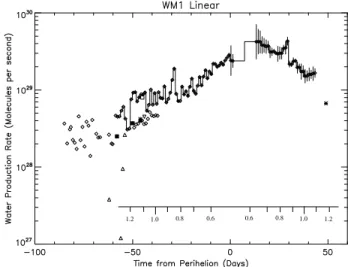
7. 2000 WM1 LINEAR
Comet 2000 WM1 LINEAR (hereafter also referred to as WM1) reached a perihelion distance of 0.555 AU on 22.6734 January (UT), 2002. SWAN observations of WM1 are available from 2001 December 10 to 2002 March 10, covering a range of heliocentric distances from 1.21 AU before perihelion to 1.12 AU after. The observational circumstances of the individual SWAN images as well as the single-image water production rates are given in Table8.
The fourth panel of Figure1shows the variation of the single-image water production rates plotted as a function heliocentric distance. While not the most productive comet of this group, WM1 had the shallowest variation with heliocentric distance with power-law exponents before and after perihelion of−1.6 and−1.1, respectively. The very shallow slope after perihelion appears to be caused by large jump in production during an unfortunate placed data gap between a few images just after perihelion and the beginning of a continuous sequence beginning at about 0.75 AU. The rest of the post-perihelion variation beginning at 0.75 AU in fact has a slope similar to the−1.4 of the pre-perihelion variation, but its value at 1 AU is more than a factor of 2 larger than before perihelion. The most likely cause of this is a seasonal variation because of a change in the orientation of the spin axis sometime during the period of January 26 and February 13. An increase such as this could be due to the first exposure of a particularly active region into the dayside hemisphere from an earlier winter polar region or a change in the projected dayside area because of a highly aspherical nucleus, i.e. the Sun exposing a long axis after perihelion but a short axis before perihelion.
Figure5shows the daily-average water production rates in C/2001 WM1 from the TRM analysis of the SWAN images plotted as a function of time from perihelion. They are listed
Table 5
Comet McNaught-Hartley: Daily-Averaged Deconvolved Water Production Rates ∆T (days) Q (s−1) ∆Q (s−1) −42.447 1.287× 1029 5.721 × 1028 −41.447 1.306× 1029 5.299 × 1028 −40.447 1.330× 1029 5.022 × 1028 −39.447 1.329× 1029 6.424 × 1028 −38.447 1.351× 1029 6.364 × 1028 −37.447 1.368× 1029 6.122 × 1028 −36.447 1.383× 1029 5.899 × 1028 −35.447 1.407× 1029 5.574 × 1028 −34.447 1.429× 1029 5.092 × 1028 −33.447 1.451× 1029 6.270 × 1028 −32.447 1.474× 1029 5.530 × 1028 −31.447 1.504× 1029 4.387 × 1028 −30.447 1.444× 1029 5.668 × 1028 −29.447 1.433× 1029 5.119 × 1028 −28.447 1.467× 1029 4.327 × 1028 −27.447 1.438× 1029 4.612 × 1028 −26.447 1.434× 1029 3.892 × 1028 −25.447 1.410× 1029 2.010 × 1028 −24.447 1.418× 1029 3.913 × 1028 −23.447 1.394× 1029 1.425 × 1028 −22.447 1.520× 1029 9.766 × 1028 −21.447 1.526× 1029 7.533 × 1028 −20.447 1.569× 1029 6.590 × 1028 −19.447 1.578× 1029 4.456 × 1028 −18.447 1.547× 1029 5.259 × 1028 −17.447 1.567× 1029 4.489 × 1028 −16.447 1.591× 1029 4.138 × 1028 −15.447 1.643× 1029 3.028 × 1028 −14.447 1.699× 1029 3.244 × 1028 −13.447 1.820× 1029 2.045 × 1028 −12.447 1.653× 1029 4.042 × 1028 −11.447 1.704× 1029 2.856 × 1028 −10.447 1.716× 1029 5.745 × 1028 −9.447 1.747× 1029 4.353 × 1028 −8.447 1.697× 1029 4.276 × 1028 −7.447 1.749× 1029 3.279 × 1028 −6.447 1.474× 1029 4.392 × 1028 −5.447 1.470× 1029 3.273 × 1028 −4.447 1.636× 1029 4.008 × 1028 −3.447 1.758× 1029 2.892 × 1028 −2.447 1.239× 1029 3.733 × 1028 −1.447 1.213× 1029 2.573 × 1028 −0.447 1.210× 1029 3.588 × 1028 0.553 1.200× 1029 2.894 × 1028 1.553 1.207× 1029 2.781 × 1028 2.553 1.266× 1029 1.783 × 1028 3.553 1.173× 1029 3.058 × 1028 4.553 1.165× 1029 2.332 × 1028 5.553 1.200× 1029 1.011 × 1028 6.553 1.207× 1029 1.092 × 1028 7.553 1.365× 1029 4.707 × 1028 8.553 1.398× 1029 4.178 × 1028 9.553 1.468× 1029 4.202 × 1028 10.553 1.519× 1029 3.280 × 1028 11.553 1.510× 1029 3.993 × 1028 12.553 1.568× 1029 2.661 × 1028 13.553 1.326× 1029 5.312 × 1028 14.553 1.256× 1029 4.549 × 1028 15.553 1.264× 1029 4.585 × 1028 16.553 1.271× 1029 3.894 × 1028 17.553 1.204× 1029 4.432 × 1028 18.553 1.227× 1029 3.301 × 1028 19.553 1.036× 1029 4.079 × 1028 20.553 9.953× 1028 3.612 × 1028 21.553 9.703× 1028 3.073 × 1028 Table 5 (Continued) ∆T (days) Q (s−1) ∆Q (s−1) 22.553 9.260× 1028 2.340 × 1028 23.553 1.022× 1029 2.497 × 1028 24.553 1.008× 1029 1.665 × 1028 25.553 9.774× 1028 2.760 × 1028 26.553 9.523× 1028 1.626 × 1028 27.553 1.005× 1029 2.957 × 1028 28.553 1.023× 1029 2.301 × 1028 29.553 9.658× 1028 2.858 × 1028 30.553 9.781× 1028 2.290 × 1028 31.553 1.019× 1029 1.799 × 1028 32.553 1.044× 1029 1.127 × 1028 33.553 9.820× 1028 1.592 × 1028 34.553 1.057× 1029 3.240 × 1026 35.553 9.015× 1028 1.889 × 1028 36.553 9.360× 1028 1.169 × 1028 37.553 8.765× 1028 1.151 × 1028 38.553 8.879× 1028 6.026 × 1027 39.553 8.831× 1028 1.562 × 1028 40.553 8.820× 1028 8.978 × 1027 41.553 9.598× 1028 2.202 × 1028 42.553 1.022× 1029 1.261 × 1028 43.553 8.241× 1028 2.208 × 1028 44.553 8.365× 1028 1.693 × 1028 45.553 8.266× 1028 1.930 × 1028 46.553 8.442× 1028 1.425 × 1028 47.553 7.985× 1028 1.809 × 1028 48.553 8.271× 1028 1.032 × 1028 49.553 7.886× 1028 1.891 × 1028 50.553 8.121× 1028 1.063 × 1028 51.553 8.012× 1028 1.571 × 1028 52.553 8.222× 1028 8.132 × 1027 53.553 7.603× 1028 1.798 × 1028 54.553 7.807× 1028 1.113 × 1028 55.553 7.284× 1028 2.243 × 1028 56.553 7.511× 1028 1.637 × 1028 Notes.
∆T: time from perihelion 2000 December 13, in days for each deconvolved value.
Q: water production rates for each image (s−1). ∆Q: 1σ formal uncertainty (s−1).
in Table9. There is some evidence for a few small outbursts of water production 30 days before perihelion and then again 30 days after perihelion, but otherwise the daily-average values follow the pre- and post-perihelion trends in the single-image values. Also shown in the figure are water production rates from a number of other investigators using different emissions from water and water by-products. The SWAS observations (Bensch et al.2004) partially overlap the early pre-perihelion coverage by SWAN and precede it by three weeks. The values are consistent but generally at the low side of the scatter in the SWAN values from−60 to −35 days and extend the apparent trend in the SWAN results to the earlier times. One value from Schleicher (a private communication reported by Irvine et al.2003) from ground-based OH photometry 46 days before perihelion is consistent with the nearby SWAN values. Radio measurements of OH by Biver et al. (2006) are also consistent with SWAS (and the lower range of the SWAN results) in the early pre-perihelion period, as are OH observations from the HST reported by Weaver et al. (2002) and water from ODIN (Lecacheux et al.2003). One of the results of OH radio measurements by Lovell et al. (2008) 54 days before perihelion is consistent with the rest, but three other earlier values fall factors of several below.
Table 6
Comet (LINEAR) A2: Observational Circumstances and Single-Image Water Production Rates
∆T (days) r (AU) ∆ (AU) g (s−1) Q (s−1) ∆Q (s−1)
−61.000 1.360 0.946 0.002439 1.281× 1029 6.364× 1025 −58.343 1.324 0.942 0.002438 1.967× 1029 5.077× 1025 −55.614 1.287 0.938 0.002437 2.085× 1029 5.041× 1025 −54.559 1.273 0.936 0.002437 2.120× 1029 5.099× 1025 −53.175 1.254 0.933 0.002436 1.688× 1029 5.381× 1025 −51.495 1.232 0.930 0.002436 1.426× 1029 7.498× 1025 −49.448 1.205 0.925 0.002409 8.962× 1028 1.106× 1026 −47.537 1.180 0.919 0.002409 5.900× 1028 1.733× 1026 −33.256 1.003 0.859 0.002333 4.699× 1028 1.470× 1026 −30.235 0.969 0.841 0.002311 5.882× 1028 1.071× 1026 −27.456 0.940 0.822 0.002289 8.120× 1028 9.265× 1025 −26.067 0.925 0.812 0.002289 8.420× 1028 8.933× 1025 −23.054 0.896 0.789 0.002268 1.136× 1029 6.479× 1025 −21.006 0.878 0.772 0.002248 1.438× 1029 6.279× 1025 −19.097 0.862 0.756 0.002229 1.418× 1029 5.314× 1025 −16.084 0.839 0.728 0.002195 1.493× 1029 5.592× 1025 −14.907 0.830 0.717 0.002181 1.602× 1029 1.110× 1025 −14.035 0.825 0.708 0.002168 1.505× 1029 5.580× 1025 −5.397 0.786 0.616 0.002106 1.813× 1029 4.293× 1025 −1.744 0.779 0.575 0.002087 1.910× 1029 3.819× 1025 −0.440 0.779 0.559 0.002083 1.975× 1029 8.121× 1024 0.298 0.779 0.551 0.002083 2.304× 1029 2.766× 1025 2.341 0.780 0.527 0.002080 2.421× 1029 2.475× 1025 5.568 0.786 0.489 0.002074 1.910× 1029 3.036× 1025 6.386 0.788 0.479 0.002076 2.012× 1029 7.954× 1024 7.637 0.793 0.465 0.002076 1.935× 1029 3.000× 1025 9.707 0.801 0.441 0.002077 1.963× 1029 2.798× 1025 12.395 0.815 0.410 0.002086 2.081× 1029 2.473× 1025 13.141 0.819 0.402 0.002093 2.210× 1029 5.635× 1024 14.465 0.828 0.388 0.002102 2.133× 1029 2.238× 1025 16.396 0.841 0.367 0.002111 1.943× 1029 2.577× 1025 18.147 0.854 0.349 0.002122 1.947× 1029 5.473× 1024 26.503 0.930 0.277 0.002172 1.744× 1029 2.215× 1025 27.126 0.936 0.273 0.002172 1.811× 1029 4.523× 1024 28.573 0.951 0.264 0.002186 1.417× 1029 2.456× 1025 30.515 0.972 0.254 0.002201 1.418× 1029 2.272× 1025 33.560 1.007 0.244 0.002200 9.531× 1028 2.889× 1025 36.099 1.036 0.241 0.002215 9.466× 1028 2.945× 1025 37.117 1.049 0.241 0.002214 8.754× 1028 6.652× 1024 38.031 1.060 0.242 0.002232 8.029× 1028 3.187× 1025 40.742 1.093 0.248 0.002231 5.206× 1028 3.660× 1025 41.865 1.107 0.253 0.002230 5.168× 1028 3.522× 1025 42.921 1.120 0.258 0.002230 4.564× 1028 3.809× 1025 44.198 1.137 0.265 0.002248 5.676× 1028 7.923× 1024 45.005 1.147 0.270 0.002247 6.101× 1028 3.918× 1025 46.765 1.170 0.282 0.002246 6.933× 1028 1.414× 1024 48.612 1.194 0.297 0.002245 6.801× 1028 6.197× 1024 49.187 1.202 0.302 0.002245 6.216× 1028 8.003× 1024 51.922 1.238 0.328 0.002263 5.463× 1028 4.038× 1025 53.460 1.258 0.344 0.002262 5.617× 1028 8.362× 1024 54.944 1.278 0.360 0.002261 4.083× 1028 5.015× 1025 55.481 1.285 0.366 0.002261 4.483× 1028 2.086× 1025 56.922 1.305 0.383 0.002260 3.289× 1028 5.780× 1025 57.453 1.312 0.389 0.002260 4.120× 1028 2.301× 1025 58.918 1.332 0.407 0.002259 3.445× 1028 5.918× 1025 59.425 1.339 0.413 0.002259 3.830× 1028 2.644× 1025 61.370 1.365 0.438 0.002258 3.462× 1028 2.306× 1025 62.252 1.377 0.449 0.002258 3.302× 1028 8.194× 1025 63.342 1.392 0.464 0.002257 3.115× 1028 3.510× 1025 64.227 1.404 0.476 0.002257 3.097× 1028 9.048× 1025 64.906 1.414 0.485 0.002256 2.698× 1028 5.570× 1024 Notes.
∆T: time from perihelion 2001 May 24, in days for each SWAN image; r: heliocentric distance (AU);∆: geocentric distance (AU); g: solar Lyman-α g-factor (photons s−1); Q: water production rates for each image (s−1);∆Q: 1σ formal uncertainty (s−1).