HAL Id: hal-00305122
https://hal.archives-ouvertes.fr/hal-00305122
Submitted on 25 Jan 2008
HAL is a multi-disciplinary open access
archive for the deposit and dissemination of
sci-entific research documents, whether they are
pub-lished or not. The documents may come from
teaching and research institutions in France or
abroad, or from public or private research centers.
L’archive ouverte pluridisciplinaire HAL, est
destinée au dépôt et à la diffusion de documents
scientifiques de niveau recherche, publiés ou non,
émanant des établissements d’enseignement et de
recherche français ou étrangers, des laboratoires
publics ou privés.
use evolution and future land use scenarios under
climate change conditions
R. Quilbé, A. N. Rousseau, J.-S. Moquet, S. Savary, S. Ricard, M. S. Garbouj
To cite this version:
R. Quilbé, A. N. Rousseau, J.-S. Moquet, S. Savary, S. Ricard, et al.. Hydrological responses of a
watershed to historical land use evolution and future land use scenarios under climate change
condi-tions. Hydrology and Earth System Sciences Discussions, European Geosciences Union, 2008, 12 (1),
pp.101-110. �hal-00305122�
Hydrol. Earth Syst. Sci., 12, 101–110, 2008 www.hydrol-earth-syst-sci.net/12/101/2008/ © Author(s) 2008. This work is licensed under a Creative Commons License.
Hydrology and
Earth System
Sciences
Hydrological responses of a watershed to historical land use
evolution and future land use scenarios under climate change
conditions
R. Quilb´e, A. N. Rousseau, J.-S. Moquet, S. Savary, S. Ricard, and M. S. Garbouj
Institut National de la Recherche Scientifique – Centre Eau, Terre et Environnement (INRS-ETE), Universit´e du Qu´ebec, 490 rue de la Couronne, Qu´ebec (QC), Canada, G1K 9A9
Received: 22 March 2007 – Published in Hydrol. Earth Syst. Sci. Discuss.: 5 June 2007 Revised: 1 October 2007 – Accepted: 10 December 2007 – Published: 25 January 2008
Abstract. Watershed runoff is closely related to land use
but this influence is difficult to quantify. This study focused on the Chaudi`ere River watershed (Qu´ebec, Canada) and had two objectives: (i) to quantify the influence of historical agri-cultural land use evolution on watershed runoff; and (ii) to assess the effect of future land use evolution scenarios under climate change conditions (CC). To achieve this, we used the integrated modeling system GIBSI. Past land use evolution was constructed using satellite images that were integrated into GIBSI. The general trend was an increase of agricultural land in the 80’s, a slight decrease in the beginning of the 90’s and a steady state over the last ten years. Simulations showed strong correlations between land use evolution and water dis-charge at the watershed outlet. For the prospective approach, we first assessed the effect of CC and then defined two oppo-site land use evolution scenarios for the horizon 2025 based on two different trends: agriculture intensification and sus-tainable development. Simulations led to a wide range of results depending on the climatologic models and gas emis-sion scenarios considered, varying from a decrease to an in-crease of annual and monthly water discharge. In this con-text, the two land use scenarios induced opposite effects on water discharge and low flow sequences, especially during the growing season. However, due to the large uncertainty linked to CC simulations, it is difficult to conclude that one land use scenario provides a better adaptation to CC than an-other. Nevertheless, this study shows that land use is a key factor that has to be taken into account when predicting po-tential future hydrological responses of a watershed.
Correspondence to: A. N. Rousseau
1 Introduction
Runoff and water quality are influenced by many natural and anthropogenic factors that occur at the watershed scale. It is well known that land use constitutes one of these factors, and that deforestation of one piece of land for agricultural or urban development can affect locally water balance and pollutant fate. This influence of land use is difficult to quan-tify, especially over the long term and at large scale such as that of a regional watershed where complex interactions oc-cur. Recent developments of decision support systems based on geographic information systems (GIS) and distributed hy-drological models have provided practical and useful tools to achieve this goal (Fohrer et al., 2001). All the studies based on such models show that deforestation for agricultural land or urbanisation induces an increase in water discharge and peak flow, but with various intensities. For instance, Costa et al. (2003) showed that increase of agricultural land from 30% to 49% of the Tocatins River watershed (Brazil, 767 000 km2) led to a 24% increase of the mean annual wa-ter discharge. On the other hand, Fohrer et al. (2001) found only a moderate effect of land use changes on the annual water balance of the small Dietzh¨olze watershed (Germany, 82 km2). Moreover, Dunn and MacKay (1995) showed, us-ing the distributed SHETRAN model, that land use change has more influence on lowland subwatersheds than on high-land subwatersheds. Thus, the intensity of the effect of land use on water regime depends on the size, the slope and land use characteristics of the watershed (see also Cognard-Plancq et al., 2001; Matheussen et al., 2000). Obviously, it also depends on the hydrological model used and the phys-ical processes simulated. Note that it is also possible to use decision support systems based on GIS and distributed hy-drological models to define an optimal land use change that would enable to achieve a specific objective such as reducing peak flow or nonpoint source pollution (Yeo et al., 2004).
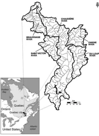
Fig. 1. The Chaudi`ere River watershed.
Assessment of land use effect on hydrology is of special interest regarding the expected climate changes (CC). In-deed, most of the studies that have tried to forecast the ef-fect of CC on hydrology and water quality consider that the watershed configuration would stay the same in the future as today (for instance Wood and Maurer, 2002). However, it is likely that land use will continue to evolve over the next decades, notably as an adaptation to CC and to regional and world economies, and that it will have an important influence on future watershed hydrology (Kite, 1993).
In this study, we used the integrated modeling system GIBSI (see description below) to assess the effect of agri-cultural land use on the hydrology of the Chaudi`ere River watershed (Qu´ebec, Canada), both under past and future con-ditions. Indeed, it is important to understand what happened in the past before trying to assess what would be the role and influence of both CC and land use evolution on future watershed hydrology (Crooks and Davies, 2001). Note that GIBSI has already been used to assess the effect of clear cut-ting on watershed hydrology (Lavigne et al., 2004) leading to consistent results. The first part of this study consists in de-termining the land use changes over the Chaudi`ere River wa-tershed between years 1970 and 2003 using remote sensing. The resulting land use maps will be compared and finally
introduced in the geographic database of GIBSI to assess the impact of land use evolution on hydrological regime. Then, the second part of the study focuses on defining land use evo-lution scenarios and simulating their influence on hydrology under future climatic conditions.
2 GIBSI
GIBSI is an integrated modelling system designed to assist stakeholders in decision making process for water manage-ment at the watershed scale (Rousseau et al., 2000; Vil-leneuve et al., 1998). It is basically composed of a MySQL® database management server, a GIS and a graphical user interface (GUI). The modeling part is based on the semi-distributed, physically based hydrological model HYDRO-TEL (Fortin et al., 2001a). HYDROHYDRO-TEL integrates six com-putational modules that are run in a cascade (i.e. in a decou-pled manner): weather data interpolation, snow cover dy-namic, potential evapotranspiration, soil moisture balance, surface runoff and streamflow. Each module offers more than one computational algorithm based on the availability of data for the studied watershed. Some algorithms, devel-oped from physically based principles, retain some empirical aspects while others are still fully empirical. Rainfall–runoff processes can be modeled on a 3–24-h time step basis. The hydrological model is sensitive to land use configuration by the mean of the Manning coefficient (for surface runoff rout-ing), leaf area index and root depth (for actual evapotranspi-ration calculation). Other models can be used (i.e. erosion, nitrogen, phosphorus and pathogens transport), but they were not considered in this study. All models run on a daily time step with meteorological data (precipitation, minimum and maximum temperatures) as inputs. Outputs are daily stream-flow and water quality data at any computational river seg-ment. Pre- and post-processing tools enable to easily define management scenarios, run simulations and analyse results. The 1995 land use configuration is used by default in the database and for simulations. It was determined based on a satellite image processed and validated with 1994 survey data (Villeneuve et al., 1998).
3 The Chaudi`ere River watershed
The Chaudi`ere River watershed is located south of Quebec City and covers an area of 6 682 km2(Fig. 1). It was selected because it is representative of many watersheds of the Saint-Lawrence River valley, with various land uses: 63% forest, 17% agricultural land, 15% bush, 3% urban development and 2% surface water. Soils vary from loam in the upper part of the watershed to clay loam in the middle part and loamy sand in the lower part. Agriculture is dominated by animal production, especially pig and dairy farming. This implies that most of farmed lands are forages and pasture (75% of agricultural land in 1995). The population of the watershed
R. Quilb´e et al.: Influence of historical and future land use on hydrology 103
Table 1. Satellite images used for the characterisation of land use evolution on the Chaudi`ere River watershed.
Acquisition date Satellite and Sensor 4 Sep 1976 Landsat-2 MSS 14 Sep 1981 Landsat-2 MSS 6 Sep 1987 Landsat-5 TM 29 July 1990 Landsat-5 TM 28 Aug 1995 Landsat-5 TM 14 July 1999 Landsat-7 ETM+ 2 Sep 2003 Landsat-5 TM+
is around 180 000 inhabitants. For the application of GIBSI, the study watershed was subdivided into 1870 elementary basins or spatial simulation units (SSUs, with a mean area of 3.6±1.9 km2), 10 lakes (5.6±8.3 km2), 1799 river segments (1.9±1.2 km), and 46 lake segments (1.5±4.4 km). Calibra-tion of the hydrological model HYDROTEL was performed on the whole watershed considering measured and simulated streamflows (for details, see Fortin et al., 2001b). The model efficiency was satisfactory regarding streamflow at the out-let of the watershed with Nash-Sutcliffe (NS) coefficients of 0.88 and 0.83 for 1989–1990 and 1993–1994, respectively. A temporal validation was performed on 1987–1988 and 1990– 1991 (NS=0.83 for both periods) as well as over a 10-year pe-riod (NS=0.89). A spatial validation was also performed for the Famine and Beaurivage subwatersheds with similar re-sults (NS between 0.78 and 0.88). Additionally, snow survey data were compared to water-equivalent depths of the sim-ulated snowpack for several stations, showing that snow ac-cumulation and snowmelt were well simulated by the model. Several management-oriented applications of GIBSI on the Chaudi`ere River watershed have been performed over the last ten years and are described by Quilb´e and Rousseau (2007).
4 Data and methods
4.1 Effect of historical land use evolution 4.1.1 Past land use evolution reconstruction
This part of this study is described in details by Savary et al. (2008)1. Identification of land use evolution was based on seven Landsat satellite images acquired over the 1970–2003 period (Table 1). Their selection was based on several cri-teria such as the period of the year (summer period is better
1Savary, S., Rousseau, A.N. and Quilb´e, R. : Assessing the
im-pact of past land use changes on runoff and low flows using remote sensing and distributed hydrological modeling – a case study for the Chaudi`ere River watershed (Quebec, Canada), in preparation, 2008.
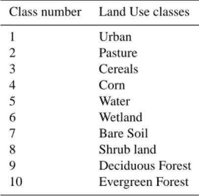
Table 2. Land use classes used in GIBSI. Class number Land Use classes
1 Urban 2 Pasture 3 Cereals 4 Corn 5 Water 6 Wetland 7 Bare Soil 8 Shrub land 9 Deciduous Forest 10 Evergreen Forest
for crop identification) and watershed cover. The image pro-cessing methodology includes three steps: pre-propro-cessing, classification and analysis. Pre-processing operations are es-sential for exploiting satellite products and allowing the ana-lyst to work within a geo-referenced environment and to re-store image quality. They include radiometric and geomet-ric transformations, as well as image resizing for the water-shed area. Classification started with the identification of clouds and water classes using mask application. Then, a supervised object-oriented classification was performed us-ing eCognition (Definens Imagus-ing, 2001) which considers not only pixel spectral characteristics but also forms, textures and neighbourhood notions. As field land use knowledge was not available, training site definition was mainly supported by visual image interpretation and previous studies on the Chaudi`ere River watershed (Dolbec et al., 2005; Gauthier, 1996). Finally, correction of unclassified regions was made using the nearest date class availability. The resulted land use classes are presented in Table 2.
4.1.2 Effect on hydrology
The classified images were integrated into GIBSI by auto-matic updating of the relevant land use tables of the database. For each land use configuration, simulations were run using measured meteorological sequences over 30 y (1970–1999) as input, each year being simulated independently. This en-sures that the results are representative of a wide range of meteorological conditions and that the differences obtained are only due to the differences in land use. Results include daily streamflow series at any computational river segment of the Chaudi`ere River watershed. We checked the effect at the watershed outlet as it integrates the effect of both land use evolution and climate change over the whole watershed. 4.2 Effect of future land use evolution
This prospective approach had to take into account not only potential evolution of land use in a near future, but also the
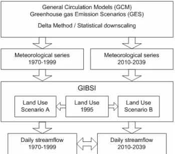
Fig. 2. General approach used to assess the effect of CC and land use evolution scenarios on hydrology.
evolution of climate. The time interval considered in this study is 30 y, the reference period being from 1970 to 1999 and the future period from 2010 to 2039. The choice of a short term prediction implies that modeled changes in wa-tershed hydrology will be slight but avoids a too important uncertainty in climate change and especially agricultural evo-lution prediction. It reflects the difficulty to determine long-term agricultural land use and world market scenarios. As stated by Butcher (1999), it is impossible to develop realistic land use projections for a period of more than 20 to 30 y. The general approach is depicted on Fig. 2.
4.2.1 Determination of future meteorological series The meteorological variables that have to be determined for the future period are the input variables of the semi-distributed hydrological model HYDROTEL which are daily minimum temperature (TMIN), maximum tempera-ture (TMAX) and precipitation (P ). Several methods ex-ist, the most popular being the use of General Circulation Models (GCMs) based on greenhouse gas emission scenar-ios (GES). GCMs accurately predict climatic variables such as wind and temperature at a large scale. However, hydrol-ogy depends on meteorological variables such as precipita-tion, minimum and maximum temperatures or evapotranspi-ration, at the land surface level and at fine spatial and tem-poral scales (Xu, 1999). To fill this gap and determine future local meteorological sequences from GCM output, we used two methods: (1) delta (or incremental) method and (2) sta-tistical downscaling (SD). Delta method is simply based on the calculation of a monthly deviation between GCM out-puts for future and present periods. SD method is more so-phisticated. The idea here is to link regional-scale climatic
Table 3. GCMs-GES-M combinations used with the two methods for determining future meteorological series.
GCM GES Member Method 1 Method 2 Method 3
CGCM3 A2 1 x 2 3 B1 1 2 3 x HadCM3 A2 a x x x b x c B2 a x x x b ECHAM4 A2 – x B2 – x
variables (so-called predictors) to local meteorological vari-ables (so-called predictands, here surface temperature and precipitation) by regression, and then to calculate future daily values of predictands based on future GCM outputs for pre-dictors. Note that a third method combining the delta method with the downscaled data was also used for comparison pur-poses, but results will not be presented here (see Quilb´e et al. (2008) for details about these three methods). For the delta method, several GCMs and GESs were available. We selected the three GCMs that gave the best results as com-pared to measured data over the reference period: (i) the third version of the Coupled General Circulation Model (CGCM3) from the Canadian Centre for Climate Modelling and Analy-sis – this version is based on CGCM2 (Flato et al., 2000) and incorporates a new version of the atmospheric component as described by Scinocca and McFarlane (2004); (ii) the third version of the Hadley Centre for Climate Prediction and Re-search model HadCM3 (Johns et al., 2001); and (iii) the Max Planck Institute for Meteorology model ECHAM4 (Roeck-ner et al., 1996). Several GESs can be considered for each GCM, as reported in the Special Report on Emission Sce-narios (SRES). Basically, sceSce-narios of families A2 and B2 correspond to pessimistic and optimistic GES, respectively. For each scenario family, several simulation members (M) are available and characterized by different initial conditions (for instance A2-a & A2-b). We selected the GES-M com-binations that gave the largest range of future meteorological conditions (see Table 3). For the SD method, the only avail-able GCM was HadCM3, based on two GESs (see Tavail-able 3). The SD procedure was performed using SDSM (Wilby et al., 2002) for nine meteorological stations out of the 40 available stations. More details about methods and results are given by Quilb´e et al. (2008).
R. Quilb´e et al.: Influence of historical and future land use on hydrology 105 Scenario B 4% 4% 0% 2% 2% 2% 5% 74% 7%
Urban Pasture Cereals Corn Water Wetland Bare soil Shrub land Forest Base case scenario (1995)
4% 11% 4% 0% 2% 2% 2% 13% 62% Scenario A 4% 14% 8% 3% 2% 2% 6% 4% 57% Forest
Fig. 3. Distribution of land use on the watershed for base case sce-nario, Scenario A and Scenario B.
4.2.2 Land use evolution scenarios
The base case scenario regarding land use was the 1995 con-figuration. Then, two opposite scenarios of future land use evolution were defined to represent a wide range of possible configurations, scenarios A and B.
– Scenario A was based on the assumption that pig
pro-duction will remain the priority incentive of agricul-tural development in the region. Thus, the evolution of pig production over the last 30 y was extrapolated to the next 20 y, from 89 739 animal units in 1995 to 136 370 animal units in 2025 (1 animal unit corresponds to 30.3 pigs). As a consequence of this increase, land use was adjusted. Indeed, increased pig production im-plies conversion of more agricultural land for pig food production (that is grain corn) and manure spreading, to the detriment of cereals, pasture, shrub land and for-est areas. Three land use classes were found to be correlated with pig production over the past 30 years: corn (r=0.76), pasture (r=0.79) and forest (r=−0.77). Then, the future class areas were extrapolated based on regression curves and future pig production.
– Scenario B was based on the assumption that
agricul-ture will make a radical change and come back to the land use configuration of 1976, with reforestation to the detriment of shrub land and pasture. This scenario also considered a spatial dispersion of corn and cereal lands over the whole watershed.
For both scenarios, the shrub land class is used as a buffer class to implement deforestation or reforestation. For sce-nario A, we make the assumption that, as most of these lands were farmed in the 70s, they are the most likely to be farmed again. Thus, new corn fields replaced shrub land and then forest area when there is no more shrub land. For scenario B, we considered that these lands will naturally transform into young forests. Note that urban area is considered to stay the same as today. These changes were integrated into GIBSI using the land use management GUI. One limitation of this system is that, for a given spatial management unit (water-shed, subwater(water-shed, municipality or SSU), every change in
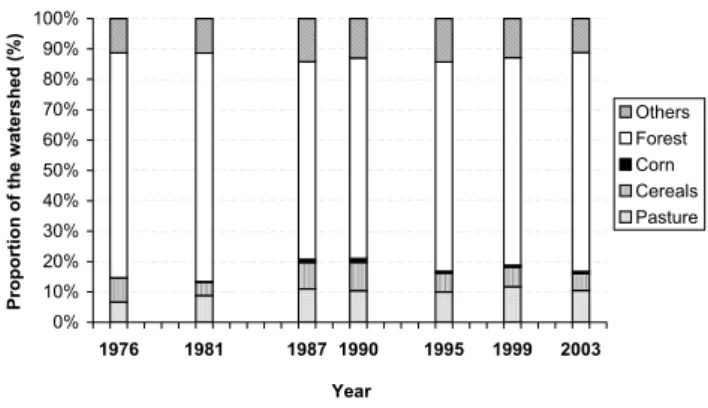
0% 10% 20% 30% 40% 50% 60% 70% 80% 90% 100% 1976 1981 1987 1990 1995 1999 2003 Year Pr o p o rti o n o f th e w a te rs h e d (% ) Others Forest Corn Cereals Pasture
Fig. 4. Evolution of agricultural and forest land use on the Chaudi`ere River watershed over the past 30 y.
land use is done by a complete transfer of one class to an-other. Therefore, we made a calculated number of transfers on different SSUs (for example all forest transformed into shrub land on one SSU, and all pasture transformed into corn on another SSU) so that the overall proportions are respected at the watershed scale. The corresponding land use distribu-tions are depicted on Fig. 3.
Note that this procedure presents some subjectivity, espe-cially in the case of scenario A. However, what is important is the general tendency at the watershed scale and the results should be considered as possible tendencies with respect to the 1995 base conditions and not be interpreted in a quanti-tative way.
4.2.3 Effect on hydrology
As indicated on Fig. 2, GIBSI simulations were performed over 30 years with original meteorological sequences (1970– 1999) and with modified (i.e. future) sequences (2010– 2039). As for the retrospective approach, each year was sim-ulated independently. This was done for each land use con-figuration (reference, scenario A and scenario B). Compar-isons between present and future watershed hydrology were made with respect to mean annual, seasonal and monthly water discharge (i.e. total runoff). In order to see the ef-fect of CC and land use evolution on low-flow events, a fre-quency analysis was performed using HYFRAN© software (Chaire en hydrologie statistique, 2002). We determined crit-ical streamflow sequences over seven and thirty consecutive days. These were Q2−7, Q10−7and Q5−30corresponding to return periods of two, ten and five years, respectively. These variables were chosen because they are used in the context of wastewater loads legislation in North America (for Q2−7 and Q10−7) and in Europe (for Q5−30). We also considered the spring peak flow. It should be noted that, by using the models under CC conditions, we may not be in the calibra-tion domain any more. Thus, we made the assumpcalibra-tion that the calibration parameter set remained optimal (Drogue et al., 2004).
460 470 480 490 500 510 520 530 540 550 560 1976 1981 1987 1990 1995 1999 2003
Land use configuration
Me a n a n n u a l w a te r d is c h a rg e (m m )
Fig. 5. Evolution of the mean annual water discharge at the outlet of the Chaudi`ere River watershed simulated with GIBSI as a function of land use configuration.
5 Results
5.1 Effect of historical land use evolution
Figure 4 presents the temporal evolution of land use over the Chaudi`ere River watershed. We can see that the agricultural land class is characterised by fluctuations attributed to the cereal class variability, while pasture area is steadier. These fluctuations of agricultural land are inversely correlated to forest evolution. This is due to the fact that new agricul-tural lands are mostly taken from shrub lands (shrub is in-cluded in the forest class), while shrub replaces agricultural lands when neglected. The mean annual runoff, simulated with GIBSI and based on 30-year meteorological series, was also found to be strongly correlated with agricultural land (r2=0.97), with a minimum of 492 mm for the 1981 land use configuration and a maximum of 555 mm for the 1990 land use configuration (see Fig. 5), and a coefficient of variation (cv) of 4.6%. Note also that the effect of land use on
wa-ter discharge is statistically significant (p<0.001, Friedmann test). It should also be noted that this effect of agricultural land on annual runoff is homogeneous over the thirty years of simulations, meaning that the relative effect is stronger for dry years. It is also important to note that this effect is more important from June to November, while there is no effect in winter and spring. Indeed, in the latter period, runoff occurs mostly under saturated soil conditions. Since evapotranspi-ration is then negligible it means that the kind of vegetation (i.e. crop type vs. forest) does not influence water balance during this period (winter and early spring). Besides, the mean spring peak flow, although correlated to land use, does not vary a lot (minimum of 1309 m3/s with the 1981 land use configuration, maximum of 1337 m3/s with the 1999 land use configuration, cv=0.8%, p<0.001). On the other hand,
in summer and fall, runoff is mainly due to strong rainfall
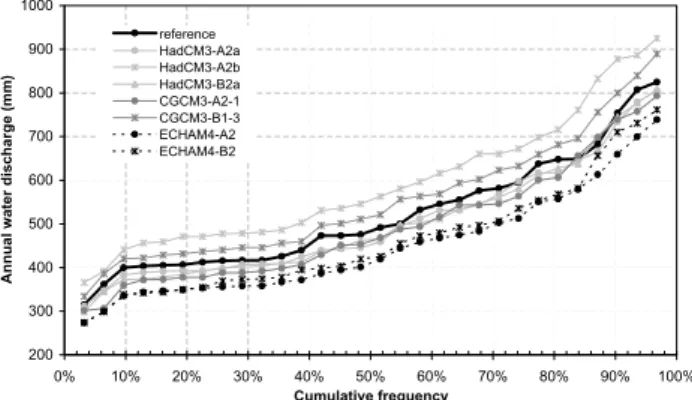
200 300 400 500 600 700 800 900 1000 0% 10% 20% 30% 40% 50% 60% 70% 80% 90% 100% Cumulative frequency A n n u a l w a te r d is c h a rg e ( m m ) reference HadCM3-A2a HadCM3-A2b HadCM3-B2a CGCM3-A2-1 CGCM3-B1-3 ECHAM4-A2 ECHAM4-B2
Fig. 6. Effect of CC on annual water discharge at the outlet of the Chaudi`ere River watershed using the delta method and the different GCM-GES-M combinations used in this study.
events, thus dense vegetation cover such as forest makes a big difference as compared to farmed land regarding rain in-terception, evapotranspiration and, consequently, runoff gen-eration. For these reasons, good correlations were also found between agricultural land and summer low flow sequences as obtained with the frequency analysis, with determination coefficients of 0.95, 0.93 and 0.93, respectively, for Q2−7, Q10−7and Q5−30. These results confirm that the hydrologi-cal regime of the Chaudi`ere River watershed is highly sensi-tive to land use.
5.2 Effect of future land use evolution under climate change
5.2.1 Effect of climate change
First, we assessed the effect of future CC on water discharge, the other factors being equal – that is considering that no change occurs in land use (i.e. 1995 configuration; that is the reference land use). Simulation results obtained with the future meteorological sequences were compared to those performed with the meteorological sequences for the refer-ence period (measured data for delta method or simulated data for SD). Figure 6 shows the annual water discharge ob-tained with the delta method (delta) using the thirty years of historical and future meteorological data. We can see an important dispersion depending on the GCM-GES-M combi-nation used. Indeed, we obtained an increase in annual water discharge for two combinations (HadCM3-A2b, CGCM3-B1-3) and a decrease for the others, especially when using ECHAM4-A2 and ECHAM4-B2. Since no GCM-GES-M combination can be determined as better than the others, this wide dispersion makes it difficult to conclude about the effect of CC on annual water discharge. One possibility is to as-sume all GCM-GES-M combinations as equiprobable. Then, the mean trend is a slight decrease of annual discharge (mean of −2.7%) which is statistically significant (p<0.01 with a paired t−test). However, the meaning of such interpretation
R. Quilb´e et al.: Influence of historical and future land use on hydrology 107 1 2 3 4 5 6 7 8 910 1112 1314 1516 1718 1920 2122 2324 0 50 100 150 200 250 W a te r d isch a rg e (mm) Month
Jan Feb Mar Apr May Jun Jul Aug Sep Oct Nov Dec * * * * * * * * * * *
Fig. 7. Monthly water discharge as simulated for reference period (left box plots) and future period with all GCM-GES-M combi-nations considered as equiprobable (right box plots). Central line indicates the median value, box-plot limits indicate 1st and 3rd quartiles, and bars indicate maximum and minimum values. Stars indicate that the means are statistically different (paired t −test,
p<0.05).
remains impossible to cast without a doubt and should be considered with caution. At the monthly time step (Fig. 7), the only effects that are observed for all GCM-GES-M com-binations were an increase in water discharge in winter (De-cember to February) and a decrease in May and October. This is in all likelihood due to the higher temperatures pre-dicted by GCMs in winter that induce less snow, more rain, and an earlier snowmelt, as well as more evapotranspiration during summer. For the other months, the effect of CC varies from one GCM-GES-M combination to another so that no general conclusion can be given, even if the means are gen-erally statistically different.
Regarding daily streamflow, results obtained with the SD method are probably more realistic than those from the delta method as the former accounts for a change in precipitation frequency and intensity while the latter does not (for a de-tailed discussion see Quilb´e et al., 2008). Unfortunately, only one GCM (HadCM3) could be considered. The results show a decrease in spring peakflow for HadCM3-A2a (−3.8% for the mean over the thirty years, not significant) and for HadCM3-B2a (−12.9%, p<0.05), due to warmer tempera-tures in winter and earlier snowmelt. Finally, regarding sum-mer low flows, results are heterogeneous. The HadCM3-A2a combination induced a strong increase in Q2−7 but a de-crease in Q5−30 and Q10−30, while HadCM3-B2a induced an increase of all sequences. It is surprising to see that the latter had a stronger effect than the former on peak flow, as GES B2 was supposed to be more optimistic regarding green-house gases emissions than GES A2. Actually, the difference
Fig. 8. Effect of land use scenarios A (middle box) and B (right box) on monthly water discharge as compared to reference land use (left box) obtained from GIBSI simulations, Delta method and two GCM-GES-M combinations (HadCM3-A2b upper graph and ECHAM4-B2 lower graph). Central line indicates the median value, box-plot limits indicate 1st and 3rd quartiles, and bars indi-cate maximum and minimum values. Stars indiindi-cate that the means are statistically different (paired t-test, p < 0.05)
between HadCM2-A2a and HadCM2-B2a is not only linked to the GES but also to different initial conditions in GES sim-ulations. Even TMIN, TMAX and P results for reference pe-riod are different for both GCM-GES-M combinations. This indicates that, at such a short term (2025), the different GES-GCM-M combinations should be seen as different, equiprob-able simulations rather than as pessimistic or optimistic con-ditions.
5.2.2 Effects of land use evolution scenarios
The previous results only accounted for the effect of CC without any change in watershed configuration. The next step was to simulate the effect of the two land use evo-lution scenarios under these CC conditions. Regard-ing the delta method, we considered here only the two GCM-GES-M combinations that gave the extreme effect on
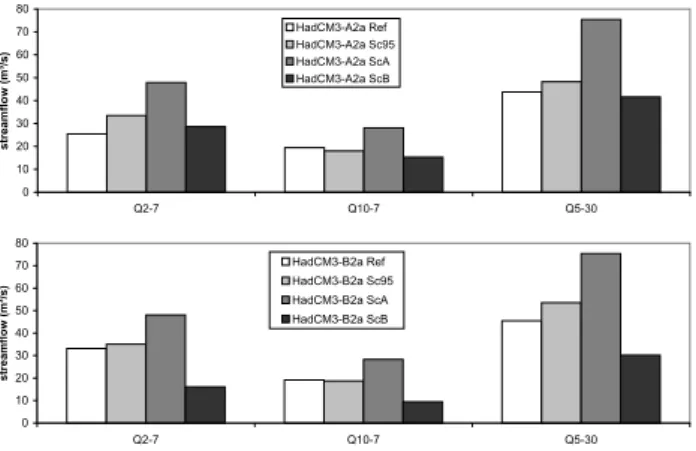
0 10 20 30 40 50 60 70 80 Q2-7 Q10-7 Q5-30 s tr e a m fl o w (m ³/ s ) HadCM3-A2a Ref HadCM3-A2a Sc95 HadCM3-A2a ScA HadCM3-A2a ScB 0 10 20 30 40 50 60 70 80 Q2-7 Q10-7 Q5-30 s tr e a m fl o w (m ³/ s ) HadCM3-B2a Ref HadCM3-B2a Sc95 HadCM3-B2a ScA HadCM3-B2a ScB
Fig. 9. Effect of CC (Sc95 vs. ref) and land use evolution sce-narios (ScA and ScB vs. Sc95) on low flow statistical sequences (m3/s) obtained with downscaling method and the two GCM-GES-M used : HadCGCM-GES-M3-A2a (upper graph) and HadCGCM-GES-M3-B2a (lower graph). “ref” is the reference simulation (reference period 1970-1999), “Sc95” stands for the future period simulation (2010-2039) considering climate change but no evolution in land use (i.e. 1995 land use) and “ScA” and “ScB” stand for the future simulations con-sidering the land use scenarios A and B, respectively, in addition to climate change.
water discharge, i.e. ECHAM4-B2 and HadCM3-A2b, as they represent the whole range of possible future conditions (see Fig. 6). The results are depicted on Fig. 8 and show that, in both cases, Scenario A would induce an important increase of water discharge from May to November, while Scenario B would induce a slight decrease over the same pe-riod. Regarding annual runoff, the effect would be +13.6% (p<0.001) and −7.2% (p<0.001), for Scenarios A and B, respectively (considering the two GCM-GES-M as equiprob-able). As shown in the first part of this study, these results are due to the strong correlation between agricultural land area and water discharge. As Scenario A includes an increase in agricultural land to the detriment of shrub land and forest, this implies an increase in runoff over the watershed in spring and fall. It is the opposite effect for Scenario B. Similar be-haviour was found regarding low flow sequences with the SD method, with an increase for Scenario A and a decrease for Scenario B. We can see on Fig. 9 that the single effect of CC on low flow sequences without any land use change (see Sc95 vs. Ref on Fig. 9) is low as compared to the effect of land use scenario A (see ScA vs. Sc95) and even scenario B for HadCM3-B2a (see ScB vs. Sc95). Note that these results are obtained from only one GCM and that other GCMs may lead to a different pattern, although it was not possible to do test these hypothesis given available data (for a complete dis-cussion regarding this methodological constraint see Quilb´e et al., 2008).
It is important to keep in mind that important uncer-tainty and many assumptions are linked to the method-ological approach that was used to determine the future
meteorological sequences. For instance, the use of ent methods (delta versus statistical downscaling) and differ-ent data sets (i.e. GCM-GES-M combinations) led to a wide range of results, some of them being contradictory. More-over, the intensity of extreme meteorological events are not well predicted by those methods, even statistical downscal-ing (Gachon et al., 2005), so that the effect on peak flow and low flow are also tainted with uncertainty. Furthermore, the hydrological model calibration was performed for a spe-cific time period and land use configuration, and we have to make the assumption that the resulting calibration parameter set remains optimal under future climate and land use con-ditions. Finally, important factors are not taken into account by this approach, such as potential implementation of irriga-tion. Consequently, it is difficult to conclude that one land use evolution scenario would be better than another under CC conditions. Bouraoui et al. (1998) performed the same kind of approach with the ANSWERS model to assess the expected effects of long term CC (doubling of CO2) and land
use management scenarios on the water balance, particularly drainage below the crop root zone. They could show that CC will induce a decrease of groundwater recharge and that this effect will be much smaller with alternative techniques such as winter wheat and/or alfalfa.
In our case, the results did not converge towards one gen-eral conclusion regarding the effect of CC on water discharge due to the large uncertainty, but they confirm the necessity to consider several sources of data. For instance, if one would have used only HadCM3-A2b to generate future meteorolog-ical sequences, he would have concluded to a strong increase of annual water discharge, while most of the other GCM-GES-M combinations predict the opposite effect. This uncer-tainty is also problematic from a management point of view. In this way, a difficult but challenging step is for scientists to communicate the results of such impact studies to stake-holders so that mitigation measures can be determined (see Fowler et al., 2007). Indeed, stakeholders need to know what will be the impact, at least a trend, so that they can make deci-sions and undertake mitigation and adaptation actions. What can be done when simulations give a wide range of possibil-ities, as it is the case here? In this regard, the quantification of uncertainty and a probabilistic risk assessment approach would be needed. Moreover, stakeholders also have to con-sider what is desirable regarding water uses. In this regard, the effect of CC and land use scenarios on pollutant loads and water quality has also to be considered as it was shown that some land use changes drastically affect many water quality parameters (Tong and Chen, 2002; Wilby et al., 2006).
In order to reduce uncertainty, further work should also use more confident techniques such as dynamical downscaling based on Regional Climate Models (for a complete overview of this modelling approach see Laprise, 2006), to predict the effect of CC in perhaps a more reliable way. However, a re-maining major problem in such studies is that, on one hand, the assessment of CC effect on hydrology has to consider
R. Quilb´e et al.: Influence of historical and future land use on hydrology 109 a long term trend (at least 2050 horizon) to produce an
ef-fect that is strong enough to be clearly related to CC and not to GCMs output variability, while on the other hand, real-istic land use evolution scenarios can only be determined at short term because of unpredictable trend in world markets (Butcher, 1999).
6 Conclusions
The first part of this study clearly shows the strong effect that land use, and especially agricultural land use, had on the hy-drological regime of the Chaudi`ere River watershed between 1970 and 1999. Therefore, as illustrated in the second part of this study, it is of major importance to take into account possible future land use evolution when forecasting the be-haviour of a watershed within a CC context (Pielke, 2005). Yet, due to the uncertainty linked to the prediction of CC ef-fect, it is difficult to conclude about the mitigation effect of the two opposite future land use scenarios considered in this study. However, they induce an effect that is in the same or-der of magnitude as – and even, in most cases, stronger than – CC on the water regime of the Chaudi`ere River during grow-ing season, confirmgrow-ing that land use will be a key factor in adaptation to CC.
Acknowledgements. This research was partly funded by a grant
from the Climate Change Action Fund (Natural Resources Canada, grant A946) and by OURANOS (Consortium on regional climatol-ogy and adaptation to climate change) (A. N. Rousseau, principal investigator). We wish to thank S´ebastien Tremblay (INRS-ETE) for precious computing help, as well as Philippe Gachon, Yonas Dibike, Nathalie Gauthier and Diane Chaumont (OURANOS) for helpful discussions and providing data.
Edited by: A. Ducharne
Reviewed by: anonymous referees
References
Arnold, J. G. and Williams, J. R.: SWRRB – A watershed scale model for soil and water resources management, in: Computer Models of Watershed Hydrology, edited by: Singh, V. P., Water Resources Publication, Highlands ranch, 847–908, 1995. Bouraoui, F., Vachaud, G., and Chen, T.: Prediction of the effect of
climatic changes and land use management on water resources, Phys. Chem. Earth, 23(4), 379–384, 1998.
Butcher, J. B.: Forecasting future land use for watershed assess-ment, J. Am. Water Resour. As., 35(3), 555–565, 1999. Chaire en hydrologie statistique: HYFRAN - Hydrological
Fre-quency Analysis, v. 1.1. INRS-ETE / HYDRO-QU ´EBEC / AL-CAN / CRSNG, 2002.
Cognard-Plancq, A.-L., Voltz, M., Didon-Lescot, J.-F., and Nor-mand, M.: The role of forest cover on streamflow down sub-Mediterranean mountain watersheds: a modelling approach, J. Hydrol., 254(1–4), 229–243, 2001.
Costa, M. H., Botta, A., and Cardille, J. A.: Effects of large-scale changes in land cover on the discharge of the Tocantins River, Southeastern Amazonia, J. Hydrol., 283(1–4), 206–217, 2003. Crooks, S. and Davies, H.: Assessment of Land Use Change in the
Thames Catchment and its Effect on the Flood Regime of the River, Phys. Chem. Earth (B), 26(7–8), 583–591, 2001. Definens Imaging: eCognition: Online user guide, available at:
http://www.definiens-imaging.com, 2001
Dolbec, J.-F., Rousseau, A. N., and Quilb´e, R.: D´eveloppement d’un process de classification d’images satellitaires afin de d´etecter les changements d’occupation du sol sur le bassin ver-sant de la rivi`ere Chaudi`ere pour la p´eriode 1970 `a 2000 : Ex-emple de l’image Landsat-5 du 6 aoˆut 1987, Report N ˚ 802, INRS-ETE, Qu´ebec, 2005.
Drogue, G., Pfister, L., Leviandier, T., El Idrissi, A., Iffly, J.-F., Mat-gen, P., Humbert, J., and Hoffmann, L.: Simulating the spatio-temporal variability of streamflow response to climate change scenarios in a mesoscale basin, J. Hydrol., 293(1–4), 255–269, 2004.
Dunn, S. M. and Mackay, R.: Spatial variation in evapotranspiration and the influence of land use on catchment hydrology, J. Hydrol., 171(1–2), 49–73, 1995.
Flato, G. M., Boer, G. J., Lee, W., McFarlane, N., Ramsden, D., and Weaver, A.: The CCCma global coupled model and its climate, Clim. Dynam., 16, 451–467, 2000.
Fohrer, N., Haverkamp, S., Eckhardt, K., and Frede, H.-G.: Hydro-logic Response to land use changes on the catchment scale, Phys. Chem. Earth (B), 26(7–8), 577–582, 2001.
Fortin, J.-P., Turcotte, R., Massicotte, S., Moussa, R., Fitzback, J., and Villeneuve, J.-P.: A distributed watershed model compati-ble with remote sensing and GIS data, Part I: Description of the model, J. Hydrol. Eng., 6(2), 91–99, 2001a.
Fortin, J.-P., Turcotte, R., Massicotte, S., Moussa, R., Fitzback, J., and Villeneuve, J.-P.: A distributed watershed model compatible with remote sensing and GIS data, Part II: Application to the Chaudi`ere watershed, J. Hydrol. Eng., 6(2), 100–108, 2001b. Fowler, H.J., Blenkinsop, S., and Tebaldi, C.: Review. Linking
cli-mate change modelling to impact studies: recent advances in downscaling techniques for hydrological modelling, Int. J. Cli-matol., 27, 1547–1578, 2007.
Gachon, P., St-Hilaire, A., Ouarda, T., Nguyen, V. T. V., Lin, C., Milton, J., Chaumont, D., Goldstein, J., Hessami, M., Nguyen, T. D., Selva, F., Nadeau, M., Roy, P., Parishkura, D., Major, D., Choux, M., and Bourque, A.: A first evaluation of the strength and weaknesses of statistical downscaling methods for simulat-ing extremes over various regions of eastern Canada, Final re-port, Sub-component, Climate Change Action Fund (CCAF), Environment Canada, Montr´eal, Qu´ebec, Canada, 2005. Gauthier, Y.: Rapport technique pr´esent´e dans le cadre de GIBSI,
Rapport technique n ˚ RT-462a, INRS-Eau, Sainte-Foy, Qu´ebec, 1996.
Johns, T. C., Gregory, J. M., Ingram, W. J., Johnson, C. E., Jones, A., Lowe, J. A., Mitchell, J. F. B., Roberts, D. L., Sexton, D. H. M., Stevenson, D. S., Tett, S. F. B., and Woodge, M. J.: An-thropogenic climate change for 1860 to 2100 simulated with the HadCM3 model under updated emissions scenarios, Hadley Cen-tre Technical Note 22, The Hadley CenCen-tre for Climate Prediction and Research, The Met Office, Bracknell, UK, 2001.
Kite, G. W.: Application of a land class hydrological model to
matic change, Water Resour. Res., 29(7), 2377–2384, 1993. Laprise, R.: Regional climate modelling, J. Comput. Phys.,
doi:10.1016/j.jcp.2006.10.024, in press, 2006.
Lavigne, M.-P., Rousseau, A. N., Turcotte, R., Laroche, A.-M., Fortin, J.-P., and Villeneuve, J.-P.: Validation and use of a dis-tributed hydrological modeling system to predict short term ef-fects of clear cutting on the hydrological regime of a watershed, Earth Interactions, 8(3), 1–19, 2004.
Matheussen, B., Kirschbaum, R. L., Goodman, I. A., O’Donnell, G. M., and Lettenmaier, D. P.: Effects of land cover change on streamflow in the interior Columbia River Basin (USA and Canada), Hydrol. Process., 14(5), 867–885, 2000.
Pielke, R. A. Sr.: Land use and climate change, Science, 310(5754), 1625–1626, 2005.
Quilb´e, R., Rousseau, A. N., Duchemin, M., Poulin, A., Gangbazo, G., and Villeneuve, J.-P.: Selecting a calculation method to esti-mate sediment and nutrient loads in streams: application to the Beaurivage River (Qu´ebec, Canada), J. Hydrol., 326, 295–310, 2005.
Quilb´e, R. and Rousseau, A. N.: GIBSI : An integrated modelling system for watershed management – Sample applications and current developments, Hydrol. Earth Syst. Sc., 11, 1785–1795, 2007.
Quilb´e, R., Rousseau, A. N., Moquet, J.-S., Trinh, N. B., Dibike, Y. B., Gachon, P., and Chaumont, D.: Assessing the effect of climate change on river flow using general circulation models and hydrological modelling. Application to the Chaudi`ere River (Qu´ebec, Canada), Can. Water Resour. J., in press, 2008. Roeckner, E., Arpe, K., Bengtsson, L., Christoph, M., Claussen,
M., D¨umenil, L., Esch, M., Giorgetta, M., Schlese, U., and Schulzweida, U.: The atmospheric general circulation model ECHAM4: model description and simulation of present-day cli-mate, 218, Max Planck Institut f¨ur Meteorology, 1996.
Rousseau, A. N., Mailhot, A., Turcotte, R., Duchemin, M., Blanchette, C., Roux, M., Etong, N., Dupont, J., and Villeneuve, J.-P.: GIBSI – An integrated modelling system prototype for river basin management, Hydrobiologia, 422/423, 465–475, 2000.
Scinocca, J. F. and McFarlane, N. A.: The variability of modeled tropical precipitation, J. Atmos. Sci., 61, 1993–2015, 2004. Tong, S. T. Y. and Chen, W.: Modeling the relationship between
land use and surface water quality, J. Environ. Manage., 66(4), 377–393, 2002.
Villeneuve, J.-P., Blanchette, C., Duchemin, M., Gagnon, J.-F., Mailhot, A., Rousseau, A. N., Roux, M., Tremblay, J.-F., and Turcotte, R.: Rapport Final du Projet GIBSI : Gestion de l’Eau des Bassins Versants `a l’Aide d’un Syst`eme Informatis´e. Mars 1998 : Tome 1., R-462, INRS-Eau, Sainte-Foy, 1998.
Wilby, R. L., Dawson, C. W., and Barrow, E. M.: SDSM – a deci-sion support tool for the assessment of regional climate change impacts, Environ. Modell. Softw., 17(2), 145–157, 2002. Wilby, R. L., Whitehead, P. G., Wade, A. J., Butterfield, D., Davis,
R. J., and Watts, G.: Integrated modelling of climate change im-pacts on water resources and quality in a lowland catchment: River Kennet, UK, J. Hydrol. 330(1–2), 204–220, 2006. Wischmeier, W. H. and Smith, D. D.: Predicting rainfall erosion
losses – A guide to conservation planning, Agricultural Hand-book No. 537, U.S. Department of Agriculture, Washington, D.C., 1978.
Wood A. W., E. P. Maurer, A. Kumar, and Lettenmaier, D.: Long-range experimental hydrologic forecasting for the eastern United States, J. Geophys. Res., 107(D20), 4429, doi:10.1029/2001JD000659, 2002.
Xu, C.-Y.: Climate Change and Hydrologic Models: A Review of Existing Gaps and Recent Research Developments, Water Re-sour. Manage., 13(5), 369–382, 1999.
Yeo, I., Gordon, S. I., and Guldmann, J. M.: Optimizing patterns of land use to reduce peak runoff flow and nonpoint source pol-lution with an integrated hydrological and land-use model, Earth Interactions, 8(6), 1–20, 2004.