Stationary and nonstationary behaviour within the geomagnetic polarity time scale

HAL Id: insu-01406447

https://hal-insu.archives-ouvertes.fr/insu-01406447

Submitted on 1 Dec 2016

HAL is a multi-disciplinary open access

archive for the deposit and dissemination of

sci-entific research documents, whether they are

pub-lished or not. The documents may come from

teaching and research institutions in France or

abroad, or from public or private research centers.

L’archive ouverte pluridisciplinaire HAL, est

destinée au dépôt et à la diffusion de documents

scientifiques de niveau recherche, publiés ou non,

émanant des établissements d’enseignement et de

recherche français ou étrangers, des laboratoires

publics ou privés.

Stationary and nonstationary behaviour within the

geomagnetic polarity time scale

Y. Gallet, G Hulot

To cite this version:

Y. Gallet, G Hulot.

Stationary and nonstationary behaviour within the geomagnetic polarity

time scale. Geophysical Research Letters, American Geophysical Union, 1997, 24, pp.1875-1878.

�10.1029/97GL01819�. �insu-01406447�

GEOPHYSICAL RESEARCH LETTERS, VOL. 24, NO. 15, PAGES 1875-1878, AUGUST 1, 1997

Stationary

and nonstationary

behaviour

within

the geomagnetic

polarity time scale

Y. Gallet and G. Hulot

D6partement

de G6omagn•tisme

et Pal•omagn•tisme

Abstract. We analyse the geomagnetic polarity time scale

(GPTS) since the Upper Jurassic by displaying the successive

lengths of polarity intervals as a function of their order of

occurrence. The sequence consists of three segments. Between

the Upper Jurassic and the Lower Cretaceous, segment "A" comprises intervals of short duration, with a mean duration of

about 0.29 My, and no clear long-term evolution. Segment

"B" begins around 130 Ma, displays a sudden increase of the

duration of the magnetic intervals, an interval of maximum duration, the normal Cretaceous superchron, and a long and erratic sequence of inteivals with decreasing average duration

between 85 Ma and about 25 Ma. From 25 Ma to the present,

segment "C" consists of intei-vais of short duration with a

mean value of 0.23 My. This description

suggests

that the

Earth's magnetic field could have experienced a fairly stationary regime until slightly befoie the onset of the

Cretaceous superchron, when the regime has been rapidly and

strongly perturbed before progressively returning to another

stationary

regime about 25 Ma ago. A geophysical

explanation for this sequence of e9ents could be that the geodynamo has been perturbed by the arrival of some cold

material at the core mantle boundary. As this material would have heated up, the geodynamo would have been brought back to its stationary regime.

1. Introduction

The origin of the numerous polarity changes of the geomagnetic field over the geological time scale is still poorly

understood. Marine magnetic anomalies clearly display large

changes in reversal frequency since the Upper Jurassic, suggesting a long time constant of about 150 My (McFadden and Merrill, 1984), and magnetostratigraphic results from the Upper Permian to the Middle Jurassic roughly confirm this suggestion since approximately 320 My (Gallet et al., 1992). This type of long-term behaviour reflects either an intrinsic property of the dynamo process itself or a response of the dynamo to some external forcing (e.g. McFadden and Merrill,

1984; 1986; Gubbins, 1987). Recently, Gallet and Courtillot

(1995)

proposed

to complete

the commonly

used

analysis

in

frequency by displaying the successive lengths of polarity

intervals as a function of their order of occurrence in the

sequence. In the present study we further consider this representation and point out that it provides new insights on the description of the GPTS since the Upper Jurassic (about

160 Ma).

Copyright 1997 by the American Geophysical Union. Paper number 97GL01819.

0094-8534/97/97GL-01819505.00

2. The GPTS as a function of order of occurence

The GPTS, which displays

no statistical

difference

between

1984; Merrill and McFadden, 1994), can be described in terms

of a Gamma process (i.e. an alteration of a Poisson process, which is a random process with no memory of its past behaviour). One can write the Gamma density probability following the convention of McFadden and Merrill (1986):

P(x)= 1 2?xt,_le_XX

(1)

where F(k) is the Gamma function of k and •, is an inherent rate of reversals associated with the unaltered Poisson process. A Gamma process reduces to a Poisson process when k is equal to one. A value for k greater than one can be interpreted either as

an artefact linked to some short intervals missing in the GPTS

or to some short term memory within the dynamo that would inhibit a second reversal just after a first ohe has occurred (McFadden and Merrill, 1993). In any case, the Gamma process describing the GPTS is known to be non stationary on time scales of 100 My, essentially because of some variation within

the inherent rate •, (k displaying little significant variations

except at the time of the Cretaceous superchron; where the reversal process seems to have been completely frozen; e.g., Merrill and McFadden, 1994).

The GPTS can therefore be viewed as the result of a time

varying Gamma process, mainly controlled by the mean

duration ],t =k/f,, an estimate of which is given by the

average

duration/,tN(i)

=(1/N)•xj of N intervals

of duration

xj

about the interval number i. This estimate, which has a

variance

Var(ktN(i))--(ktN(i)

2/kN) (McFadden,

1984),

can

be plotted

as a function

of i to characterize

the evolution

of the

We have considered a composite GPTS constituted by the Upper Cretaceous to Cenozoic polarity sequence recently proposed by Cande and Kent (1995) and the Upper Jurassic to Lower Cretaceous sequence suggested by Harland et al. (1990). The whole sequence contains 284 intervals, 99 intervals before

the Cretaceous superchron and 184 after. We acknowledge that

the uncertairities which remain in the precise absolute dates of

the Mesozoic

GPTS render

delicate

the detailed

analysis

of the

GPTS,

but we believe

that they would

not notably

modify

the

broad description we intend to do hereafter. The polarity

interval dt•rahons for both polarities are shown as a function of

order of occurrence on Figure 1. The raw data is plotted on Figure l a, and the corresponding estimates ktN(i) for N=25 on Figure lb (except when they involve the Cretaceous superchron). We have arbitrarily chosen N=25 in order to smooth most of the ambiguous short-term fluctuations. We

1876 GALLET AND HULOT: STATIONARY AND NONSTATIONARY BEttAVIOIIR

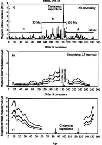
REAL DATA

a) Cretaceous

_superchron

_No

_smoothing

25

Ma

I B • I 130Ma

, , •L

,superchron

Figure 1. Polarity interval durations as a function of order of occurrence (Fig. l a,b). The first interval is Brunhes. The raw data is shown on Fig. la, and gN(i) for N=25 and k=l is plotted

with its 2(5N=25

errors

((SN(i)=gN(i)/x/N)

on Fig. lb (except

7.*50 since

approximately

160 Myr. We also

plotted

the

curves

7.+(i)=1/(g50(i)+2(550(i))

and 7._(i)=1/(g50(i)-2(550(i)

)

within

which

7.*50

is expected

to fluctuate.

also have considered k=l to compute the errors associated with

•, although k is usually slightly larger (and thus the

uncertainties smaller). Both diagrams support the idea that a

difference exists in reversal behaviour before and after the

Cretaceous

superchron

(the Cretaceous

superchron

#185 is

preceeded by only 2 intervals that last longer than 1.5 My,

whereas

at least 9 such intervals follow it; Fig. l a). They

further suggest

that the GPTS can essentially

be described

by

three segments. Between intervals #284 and #193 (segment A: Upper Jurassic-Lower Cretaceous), the magnetic reversals a/'e

of short duration

with no clear long-term

evolution,

•tN(i)

being roughly constant within error bars ([t A=0.29 _+ 0.03

My). Between intervals #192 and #110 (segment B), the

average

duration

first increases

quickly (in less than 10 My),

reaches

a maximum

with the Cretaceous

superchron

(35 My;

Cande and Kent, 1995), and then decreases

slowly between

intervals #184 and approximately #110 (from about 85 Ma to

25 Ma). A third segment (C) finally characterises intervals

#110 to #1. The magnetic

intervals

are then again of short

duration,

with gC=0.23 _+ 0.02 My. As previously

suggested,

the observed

behaviour

resembles

fiat white

noise

(Dubois

and

Painbrun, 1990; Gallet and Courtillot, 1995).

We next plotted histograms of the duration of the magnetic intervals for the 3 segments (Fig. 2a). Each number of intervals has been divided by the total number of intervals withit/the respective segment. Whereas segments A and C are indeed very similar, segment B clearly differs eventhough we did not take the onset of B and the Cretaceous superchron into

accoufit.

Plotting

histograms

of the relative

duration

of the

magnetic

intervals

with respect

to the time varying

estimate

of

[t gives a different picture (Fig. 2b). The lengths of the magnetic intervals have been divided by their respective mean duration tbr segments A (gA) and C (gC), and by a varying

valu• [t B(i) defined by a linear trend adjusted

to the one

observed

in Figur6

lb (between

the value

of 1.0 My for interval

the small riumber of intervals in each segment). This confirms

that the GPTS can be interpreted as the result of one process essentially characterized by the parameter la (except during the

onset

of B and

the Cretaceous

superchron).

3. Discussion

ß

Previous analyses have shown that the GPTS is the result of

a Gamma

process

defined

by equation

(1) and characterized

by

the two parameters

k and 7., or alternately

k and la=k/7..

Because

k clearly displays little significant

variations

through the

sequence. changes in the GPTS are essentially due to variations

either

in 7. or g. But neither

7. nor la are readily

accessible

to

r i Segment

A [

I I

0 -- 0.4 -- 0.8 -- 1.2 -- 1.6 -- 2.0 -- 2.4 -- 2.8 -- 3.2 -- 3.6 -- 4.0 Intervals of duration (My)

I .-.Y73?l Seg .... B I

• 0.3 F

I

0 .... :'•

04 08 12 16 20 24 28 32- 3.6 -4.0 Normalised intervals of duration

Figure 2. Histograms of duration of the intervals defining

the three segments A,B,C. Only the intervals following the

Cretaceous superchron have been considered for the segment

B. The histograms have been normalized to the total number of

intervals within each segment (Fig. 2a). Fig. 2b: same except

that the duration of the magnetic intervals has been divided by

GALLET AND HULOT: STATIONARY AND NONSTATIONARY BEHAVIOUR 1877

measurement. The only parameter which can be recovered with some good statistical understanding is the estimator gN(i)of g (McFadden, 1984). Plotting gN(i) as a function of i (order of occurrence) treats each realization of the process with equal weight (Fig. lb). This representation underlines the different nature of the non-stationarity of the reversal process before and after the Cretaceous superchron. It also shows the close similarity between segments A and C, together with their fiat white noise-like behaviour. This latter characteristic suggests that during the corresponding periods of time the geodynamo experienced a fairly stationary regime characterized by the random occurrence of short magnetic polarity intervals (Dubois and Pambrun, 1990; Gallet and Courtillot, 1995). The

onset of the Cretaceous superchron at the beginning of

segment B, in about 5 My (Harland et al., 1990), shows that the stationary regime defined by segment A rapidly ended

slightly before the superchron. In contrast the second part of

segment B, between 85 Ma and 25 Ma, indicates a progressive return to another stationary regime (segment C).

This interpretation of the GPTS represents an alternative to the one of McFadden and Merrill (1984) which is based on the

curve

derived

from

the

GPTS

by plotting

X*50(i)=l/g50(i)

as

a

function of the age (and no longer as a function of i). The

parameter

X*50 provides

an estimate

of ),./k

and

as

k changes

little,

variations

in X*50 can

be interpreted

as changes

in the

true reversal rate ),, (McFadden, 1984). The corresponding curve

is shown on Figure l c together with the bands within which

the

estimator

X*50 is expected

to fluctuate

about

X/k.

For

the

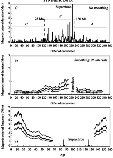
last 100 My, this curve suggests that the reversal rate has gradually increased from the end of the Cretaceous superchron to the present. This interpretation is compatible with the data but is strongly guided by the way the data is presented. The time when the process is clearly non-stationary (our segment B) corresponds to a long period on Figure l c and invites to extrapolate this behaviour up to the present. Also the choice of N=50 strongly smoothes the curve and short term changes in the trend are impossible to see (only three averages are statistically independent over the last 100 My). On the contrary, our curve (Fig. lb) closely sticks to the original data (Fig. la), involves twice less averaging and provides a better chance of assessing the non-stationarity within the GPTS. It suggests with equal statistical value that changes in behaviour could have indeed occurred about 25 Ma and 130 Ma ago. For

further confirmation, we have generated a synthetic magnetic

polarity sequence with the help of a Poisson process controlled by a parameter g equal to gA during enough intervals to cover

the length of segment A (from 160 to 130 My), stopped during

a fictitious superchon, reinitiated with g=gB(i) during the time

of segment B, and finally made stationary again with g=gc

during the time of segment C (Fig. 3). Whereas Figure 3c shows the same trends as Figure l c that led McFadden and

Merrill (1984) to their interpretation, Figure 3b properly

recovers the three segments we had input and looks very similar to Figure lb.

Interpreting the reversal behaviour in terms of physical process is notoriously speculative, because little is known about what controls the reversals. Boundary conditions imposed by the core-mantle boundary (CMB) certainly influence the geodynamo and may thus control changes in the

GPTS. Here we explicitely assume that changes in p result from

some changes within the CMB boundary conditions. The most

8

• o

c

I

I

I

Figure 3. Synthetic magnetic polarity sequence generated as

described in the text. Same representations as in Fig. 2.

important conditions are believed to be the thermal ones at the CMB which control the heat flux extracted from the core.

Gubbins (1987) pointed out the possible influence of mantle

thermal lateral variations

on the behaviour

of the magnetic

field. Stacey (1991) further suggested

that there might be

crypto-continents drafting and inducing additional lateral

thermal variations at the CMB. But changes produced in this

way are slow and can hardly account

for the rapid tYeezing

of

the reversal process in less then 10 My. Several other authors

underlined

the fact that the heat flux is controlled

by the

thickness

of the D" layer (assumed

to be a thermal

boundary

layer) at the base

of the mantle

and that this thickness

is likely

to change every time a plume erupts as a result of some

instabilities

within D" (e.g., Loper and McCartney, 1986;

Courtillot and Besse, 1987; Larson and Olson, 1991). But

Loper (1992) showed

that partially

emptying

D" only leads to

years). A plume leaving D" would therefore not better account tbr the A, B, C sequence.

In contrast,

if some

cold material

could

be brought

quickly

in direct

contact

with

the

core,

the

heat

flux

would

be

promptly

and drastically

altered.

Such

a thermal

anomaly

could

possibly

explain the sudden onset of segment B. For a slab-like structure

with a thermal

diffusivity

k=10-6m2s-1

that

arrives

in contact

with the core, the flux below this structure

is proportional

at

any subsequent

time

t to the temperature

gradient

AT/(krct)

1/2,

1878 GALLET AND HULOT: STATIONARY AND NONSTATIONARY BEHAVIOUR

and the cold anomaly (e.g., Turcotte and Schubert, 1982). This

temperature gradient goes back to a value comparable to the

one the thermal boundary layer enjoyed before the arrival of

the cold material (VT), after a relaxation time of the order of

b2/krc,

where

b=AT/VT is the distance

from the CMB within

the thermal boundary corresponding to a temperature drop of

AT. This can be assumed to be of the order of the thickness of

the thermal boundary layer itself (say 100 km). A relaxation

time of about 100 My is found, which is the order of magnitude of the duration of our segment B. A possible interpretation of

the A,B,C sequence is then that the thermal boundary

conditions could have remained stable during A, have been

perturbed at the onset of B by the arrival of some cold material

at the CMB, and have settled back as the cold material was heated back to some thermal equilibrium. The mechanism that

could push cold material at the CMB remains uncertain. An

efficient candidate could be a mantle avalanche. Indeed, 3-D numerical models of mantle convection incorporating an endothermic phase transformation at the 660 km discontinuity

all display hybrid convection. This type of convection is

mainly two-layered but occasionnally may experience flushing

events during which cold material suddenly sinks from the upper mantle into the lower mantle (e.g., Machetel and Weber,

1991). As an alternative, a subducted slab could have

penetrated into the lower mantle and landed at the CMB (e.g.,

Christensen, 1996; Eide and Torsvik, 1996). Such events seem to be rare enough to account for the fact that just one is being seen in the 160 My long GPTS, and quick enough for the

material to remain significantly cold when it reaches the CMB.

This interpretation of the GPTS assumes that reversals of the geomagnetic field are strongly inhibited by the local

increase in the heat flux associated with the arrival of cold

material at the CMB. We note that such local changes would modify the boundary conditions. Altering the boundary conditions in rotating convective systems clearly impose strong and global constraints on the nature of the solution

chosen by the system (e.g., Zhang and Gubbins, 1993). 'We

therefore suggest that these changes could prevent the system from going through intermediate states that would normally lead to a reversal. At the onset of B, the perturbation would have been particularly strong and the system would have remained stuck in one polarity. As the cold material would have progressively heated up, the perturbation would have been weaker, only proportionnally impeding the reversals. This further suggests that the size of the cold anomaly arriving at the CMB could provoke and determine the duration of the subsequent superchron. This could explain the longer duration of the Kiaman superchron occurring during the Late Paleozoic (Harland et al., 1990). This scenario does not preclude some correlations with plume eruptions possibly triggered by the

arrival of the cold material within D".

References

Cande, S., and D. Kent, Revised calibration of the geomagnetic polarity

timescale for the Late Cretaceous and Cenozoic, J. Geophys. Res., 100, 6093-6095, 1995.

Courtillot, V., and J. Besse, Magnetic field reversals, polar wander, and

Core-Mantle coupling, Science, 237, 1140-1147, 1987.

Christensen, U., The influence of trench migration on slab penetration

into the lower mantle, Earth Planet. Sci. Lett., 140, 27-39, 1996. Dubois, J., and C. Pambrun, Etude de la distribution des inversions du

champ magn6tique terrestre entre -165 Ma et l'actuel (6chelle de

Cox). Recherche d'un attracteur dans le systeme dynamique qui les g6n•re, C. R. Acad. Sci. Paris, 311,643-650, 1990.

Eide, E., and T. Torsvik, Paleozoic supercontinental assembly, mantle flushing, and genesis of the Kiaman superchron, Earth Planet. Sci.

Lett., 144, 389-402, 1996.

Gallet, Y., J. Besse, L. Krystyn, J. Marcoux, and H. Th6veniaut,

Magnetostratigraphy of the Late Triassic Bolticektasi Tepe section (northwestern Turkey): implication for changes in magnetic reversal frequency, Phys. Earth Planet. lnt., 73, 85-108, 1992.

Gallet, Y., and V. Courtillot, Geomagnetic reversal behaviour since 100 Ma, Phys. Earth Planet. lnt., 92,235-244, 1995.

Gubbins, D., Mechanism for geomagnetic polarity reversals, Nature,

326, 167-169, 1987.

Hadand, W., R. Armstrong, A. Cox, L. Craig, A. Smith, and D. Smith, A

geologic time scale, Cambridge University Press, 263 pp, 1990.

Larson, R., and P. Olson, Mantle plumes control magnetic reversal frequency, Earth Planet. Sci. Lett., 107, 437-447, 1991.

Loper, D., and K. McCartney, Mantle plumes and the periodicity of magnetic field reversals, Geophys. Res. Lett., 13, 1525-1528, 1986. Loper, D., On the correlation between mantle plume flux and the

frequency of reversals of the geomagnetic field, Geophys. Res. lett.,

19, 25-28, 1992.

Machetel, P., and P. Weber, Intermittent layered convection in a model

with an endothermic phase change at 670 km, Natttre, 350, 55-57,

1991.

McFadden, P., Statistical tools for the analysis of geomagnetic reversal

sequences, J. Geophys. Res., 89, 3363-3372, 1984.

McFadden, P., and R. Merrill, Lower Mantle convection and

geomagnetism, J. Geophys. Res., 89, 3354-3362, 1984.

McFadden, P., and R. Merrill, Geodynamo energy source constraints fi'om paleomagnetic data, Earth Planet. Sci. Lett., 42, 22-33, 1986. McFadden, P.L., and R.T. Merrill, Inhibition and geomagnetic field

reversals, J. Geophys. Res., 98, 6189-6199, 1993.

Merrill, R.T., and P.L. McFadden, Geomagnetic field stability: Reversal

events and excursions, Earth Placket. Sci. Lett., 121, 57-69, 1994.

Stacey, F., Effect on the core structure within D", Geophys. Astrophys.

Fhtid Dymtm., 60, 157-163, 1991.

Turcotte, D., and G. Schubert, Geodynamics. Applications of continuum physics to geological problems, J.Wiley and Sons eds., New York,

450 pp., 1982.

Zhang, K., and D. Gubbins, Convection in a rotating spherical fluid shell with an inhomogeneous temperature boundary condition at infinite

Prandtl number, J. Fluid. Mech., 250, 209-232,1993.

Y. Gallet and G. Hulot, IPGP, D•partement de G•omagn•tisme et

Pal•omagn•tisme, 4 Place Jussieu, 75252 Paris Cedex 05, France.

Acknowledgments. We thank J. Besse, J. Carlut, V. Courtillot, S. Gilder and L.E. Ricou for their help. IPGP Contribution no. 1480 and INSU, program "Terre Profonde" Contribution no. 87.

(Received August 14, 1996; revised March 25, 1997;