How unusual was autumn 2006 in Europe?

(1)

HAL Id: hal-00298096

https://hal.archives-ouvertes.fr/hal-00298096

Submitted on 21 Nov 2007

HAL is a multi-disciplinary open access

archive for the deposit and dissemination of

sci-entific research documents, whether they are

pub-lished or not. The documents may come from

teaching and research institutions in France or

abroad, or from public or private research centers.

L’archive ouverte pluridisciplinaire HAL, est

destinée au dépôt et à la diffusion de documents

scientifiques de niveau recherche, publiés ou non,

émanant des établissements d’enseignement et de

recherche français ou étrangers, des laboratoires

publics ou privés.

G. J. van Oldenborgh

To cite this version:

G. J. van Oldenborgh. How unusual was autumn 2006 in Europe?. Climate of the Past, European

Geosciences Union (EGU), 2007, 3 (4), pp.659-668. �hal-00298096�

(2)

Clim. Past, 3, 659–668, 2007 www.clim-past.net/3/659/2007/

Climate

of the Past

How unusual was autumn 2006 in Europe?

G. J. van Oldenborgh

KNMI, De Bilt, The Netherlands

Received: 21 May 2007 – Published in Clim. Past Discuss.: 8 June 2007

Revised: 9 October 2007 – Accepted: 5 November 2007 – Published: 21 November 2007

Abstract. The temperatures in large parts of Europe have

been record high during the meteorological autumn of 2006. Compared to 1961–1990, the 2 m temperature was more than three degrees Celsius above normal from the North side of the Alps to southern Norway. This made it by far the warmest autumn on record in the United Kingdom, Belgium, the Netherlands, Denmark, Germany and Switzerland, with the records in Central England going back to 1659, in the Nether-lands to 1706 and in Denmark to 1768. The deviations were so large that under the obviously false assumption that the climate does not change, the observed temperatures for 2006 would occur with a probability of less than once every 10 000 years in a large part of Europe, given the distribution defined by the temperatures in the autumn 1901–2005.

A better description of the temperature distribution is to assume that the mean changes proportional to the global mean temperature, but the shape of the distribution remains the same. This includes to first order the effects of global warming. Even under this assumption the autumn tempera-tures were very unusual, with estimates of the return time of 200 to 2000 years in this region. The lower bound of the 95% confidence interval is more than 100 to 300 years.

Apart from global warming, linear effects of a southerly circulation are found to give the largest contributions, ex-plaining about half of the anomalies. SST anomalies in the North Sea were also important along the coast.

Climate models that simulate the current atmospheric cir-culation well underestimate the observed mean rise in au-tumn temperatures. They do not simulate a change in the shape of the distribution that would increase the probability of warm events under global warming. This implies that the warm autumn 2006 either was a very rare coincidence, or the local temperature rise is much stronger than modelled, or non-linear physics that is missing from these models in-creases the probability of warm extremes.

Correspondence to: G. J. van Oldenborgh

(oldenborgh@knmi.nl)

1 Introduction

Meteorologically, the autumn of 2006 was an extraordinary season in Europe. In the Netherlands, the 2-m temperature

at De Bilt averaged over September–November was 1.6◦C

higher than the previous record since regular observations

began in the Netherlands in 1706, which was a tie between 1731 and 2005 (Fig. 1a). The excess is much larger than the uncertainties in the earlier part of the record: van En-gelen and Geurts (1985) estimate that the standard error of

monthly temperatures is 0.2–0.3◦C (see also van den Dool

et al., 1978). The Central England Temperature, 12.6◦C,

also was the highest since the beginning of the

measure-ments in 1659, 0.8◦C higher than the previous record of

1730 and 1731. Pre-instrumental reconstructions indicate that September–November 2006 very likely was the warmest autumn since 1500 in a large part of Europe (Luterbacher et al., 2007).

The impacts of the high temperatures on society and na-ture have not been very strong, as in autumn a higher tem-perature corresponds to a phase lag of the seasonal cycle. Flowering bulb farmers in the Netherlands were reported to have problems due to premature flowering. However, a simi-lar anomaly in summer would have given rise to a heat wave analogous to the summer of 2003, which caused severe prob-lems (e.g., Sch¨ar and Jendritzky, 2004).

In this article the heat anomaly of the autumn of 2006 in Europe is analysed. First the observations are shown and return times are computed under the obviously false assump-tion of a staassump-tionary climate. Next the first order effects of global warming are subtracted, and return times of the re-maining weather signal computed. The main weather factors are identified, and possible changes in their distribution are investigated using climate model simulations.

(3)

(a)

7 8 9 10 11 12 13 [C] 14 1700 1750 1800 1850 1900 1950 2000 2050

(b)

7 8 9 10 11 12 13 [C] 14 1900 1920 1940 1960 1980 2000 2020

Fig. 1. Autumn 2-meter temperatures at De Bilt, the Netherlands with a 10-yr running mean (green) 1706–2006 (a, van Engelen and Nellestijn, 1996), 1901–2006 corrected for changes in the ther-mometer hut, location and city effects (b, Verbeek, 2003).

7 8 9 10 11 12 13 14 10000 1000 100 10 5 2 [Celsius]

return period [yr]

Sep-Nov homogenized temperature De Bilt 1901:2005

gauss fit gpd fit 2006

Fig. 2. Extrapolation of homogenised De Bilt autumn temperatures 1901–2005 (crosses) to the value observed in 2006 (horizontal line) using a fit to a Gaussian distribution and a Generalised Pareto Distri-bution (to the highest 20%). The return times have been computed under the obviously false assumption of only interannual variability. The upper and lower lines indicate the 95% CI, determined with a non-parametric bootstrap.

2 Observations

In Fig. 1 two time series of autumn (September–November) averaged temperature in De Bilt, the Netherlands are shown. The first one covers 1706–2006 and is a combination of ob-servations at various locations in the Netherlands converted to De Bilt temperatures (van Engelen and Nellestijn, 1996). The second time series 1901–2006 has been corrected for the effects of changes in thermometer hut, direct environment of the measurement location (Brandsma and van der Meulen, 2007a,b), and the effects of the growth of the cities in the area (Brandsma et al., 2003). The value for 2006 is seen to be well outside the distribution defined by the other years in both series.

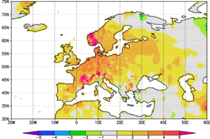
Fig. 3. The temperature anomaly (degrees Celsius) relative to 1961– 1990) of September–November 2006 in the GHCN/CAMS dataset (Fan and van den Dool, 2007).

Figure 2 shows two extrapolations of the cumulative distri-bution of the second, homogenised, time series 1901–2005, the first assuming a Gaussian (normal) distribution and the second using a peak-over-threshold method with a fit of the warmest 20% to a Generalised Pareto Distribution (GPD; Coles, 2001). These extrapolations are based on the obvi-ously false assumption that the autocorrelation is zero, i.e., that there are no long-term variations except those resulting from accumulations of interannual variability. From Fig. 2 it seems likely that the Gaussian distribution overestimates the probability of high temperatures. In spite of this a return time of 10 000 year is obtained with this extrapolation. This shows that the assumption of no autocorrelation is very likely false: climate does change on longer time scales. Physically, global warming has made high temperature anomalies much more likely during recent years, and this and other long-term vari-ations increase the probability of clustered high extremes.

The same analysis has been applied to all grid points of the

0.5◦ Global Historical Climate Network (GHCN)/Climate

Anomaly Monitoring System (CAMS) (Fan and van den Dool, 2007). The GHCN and CAMS time series used in the construction of this dataset have not been homogenised, in contrast to the De Bilt series of Fig. 1b (which is not included

in this dataset). All results have been verified against the 5◦

CRUTEM3 dataset (Brohan et al., 2006) (not shown).

Figure 3 shows that the area with 3◦_{C anomalies stretches}

from the the Alps to Denmark and from Belgium to Poland, with maxima in the the Alps and in southern Norway. An extrapolation using a Gaussian fit (Fig. 4) shows that in an unchanging climate the return times of this autumn would be 10 000 years or more in an area shifted somewhat to the west of the area with highest anomalies. (The shift is due to the smaller variability near the Atlantic Ocean.) As can also be shown directly, year-to-year autocorrelations are not negligible.

(4)

G. J. van Oldenborgh: How unusual was autumn 2006 in Europe? 661

Fig. 4. The return time (years) of September–November 2006 in the GHCN/CAMS dataset 1948–2005 under the false assumption of a stationary climate, using the more conservative Gaussian extrapola-tion.

3 Global warming

The climate is not stationary: temperatures have been rising over Europe as in most of the rest of the world (IPCC, 2007). The effect of this on the probability of the occurrence of an anomaly like in autumn 2006 can be studied in a first approx-imation by subtracting the local temperature change propor-tional to a global temperature, here the 3-yr running mean

of the global mean temperature, T_global′(3) (t ). (On interannual

time scales T_global′ (t )contains clear ENSO signals, and these

should not enter in the description of how global temperature affects Europe, hence the low-pass filtering.) This gives as a first approximation:

T′(t ) = AT_global′(3) (t ) + ǫ(t ) , (1) where ǫ(t ) denotes the part of the temperature not directly proportional to global temperature changes. The coefficients

Aare determined by a fit of local to global temperature up to

2005 and are shown in Fig. 5.

Station inhomogeneities (or local temperature anomalies) are visible in the GHCN/CAMS dataset (these are not vis-ible in the much coarser CRUTEM3 dataset). On average the temperature in Europe has increased somewhat faster than the globally averaged temperature in autumn, in ac-cordance with the Cold Ocean/Warm Land pattern (Sutton

et al., 2007). For the homogenised De Bilt time series,

A=1.68±0.37 (1σ standard error) over 1901–2005.

Subtracting the local trend AT_global′(3) (t )from the observed

temperatures, the weather anomalies ǫ(t ) remain. The

anomalies up to 2005 are described reasonably well by a Gaussian in autumn; the skewness is −0.46±0.36, so the Gaussian fit may even overestimate the positive tail. The au-tocorrelation is now slightly negative at lags up to 4 year, so

Fig. 5. The regression A of local against globally averaged tem-perature over 1948–2006. Only grid points where the correlation is 90% significant (assuming a normal distribution) are shown.

7 8 9 10 11 12 13 14 2 5 10 100 1000 10000 [Celsius]

return period [yr]

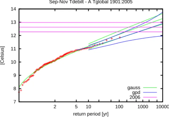
Sep-Nov Tdebilt - A Tglobal 1901:2005

gauss gpd 2006

Fig. 6. As Fig. 2 but now for T (t)−AT_global′(3) (t ), the De Bilt tem-perature with the regression against the global mean temtem-perature anomalies (with a 3-yr running mean) subtracted. The 95% un-certainty interval in the 2006 anomaly above the trend due to the uncertainty in the regression is denoted by the horizontal lines.

that consecutive years of this series can be considered inde-pendent.

In Fig. 6 the cumulative distribution of the autumn tem-peratures minus the linear effect of global mean temperature changes 1901–2005 is shown. Extrapolating this to the value observed in 2006 gives a return time of 650 years. Using a GPD to fit the highest 20% of the distribution gives a return time of about 3000 years. To compute the statistical uncer-tainty margins in these numbers a non-parametric bootstrap was performed simultaneously on the regression and the ex-trapolation. This gives a 95% CI on the return time of 125 to 10 000 years for the Gaussian extrapolation, 200 years to

(5)

(a)

(b)

Fig. 7. As Fig. 4 but now with the local linear regression against the global mean temperature anomalies (with a 3-yr running mean, Fig. 5) subtracted (a), lower bound of the 95% confidence interval on the return time (b).

(a)

(b)

(c)

Fig. 8. NCEP/NCAR sea-level pressure anomalies (hPa) relative to 1961-1990 in September (a), October (b) and November 2006 (c). The black lines indicate the number of standard deviations of the anomaly.

infinity for the GPD extrapolation. The lower bounds are reached when the real trend is higher than the central fitted value of A=1.68, lowering the value for 2006 (lower hori-zontal line).

The same extrapolation in the GHCN/CAMS dataset (Fig. 7) show the improbable weather to have extended over a large part of Europe, with estimates of return times of

ǫ(t )longer than 200 years over most of the area where the anomaly was largest, reaching 2000 years in northern Ger-many. The lower bounds of the two-sided 95% confidence interval (determined as in Fig. 6) are more than 300 years there. The Gaussian approximation probably underestimates the return times, as the anomalies ǫ(t ) are negatively skewed in most of the area.

We conclude that global warming has made a temperature anomaly like the one observed in autumn 2006 between 10 and 50 times more likely than under the false assumption of stationary climate, with the larger factors near coasts where the trend is larger compared to natural variability. Still, other factors than global warming conspired to give estimated

re-turn times well over 200 years in most of the area with large anomalies, reaching 2000 years (lower bound 300 years) in northern Germany. A rare event indeed, even taking into ac-count a shift in the probability density function proportional to global temperature changes, determined over the period before 2006.

4 Circulation

It is obvious that a large part of the temperature anomalies in autumn 2006 was caused by the abnormal circulation in these months. A persistent low-pressure area over the At-lantic Ocean caused predominantly south-easterly winds in September, southerly winds in October and south-westerly winds in November to the area north of the Alps (Fig. 8). In each of these months this corresponded to the direction advecting the highest temperatures.

The question how unusual the circulation patterns were

is not easy to answer. The local pressure anomalies did

(6)

(a)

(b)

(c)

(d)

Fig. 9. The coefficients of the VSM Eqs (2-4) averaged over September-November: zonal geostrophic wind AW[Km−1s] (a), the meridional

zonal wind A_S[Km−1s] (b), the vorticity B[K hPa−1](c); the memory term M [1] in September (d).

Fig. 10. Correlation of the September–November temperature anomaly from the VSM with η(t)=0 and the observed temperature 1948–2005.

lines in Fig. 8). A deviation of this size is not rare without restriction on the location.

In order to do a meaningful extreme value analysis on the circulation patterns these 2-dimensional fields have to be re-duced to local time series. One way to do this is to compute a circulation-dependent temperature. In Europe, temperatures are determined to a large extend by wind direction due to large climatological temperature gradients. Cloudiness also affects the temperature independently. In the very simple model (VSM) of van Ulden and van Oldenborgh (2006) the anomaly in local monthly mean 2 m temperature is therefore decomposed as

T′(t ) = T_circ′ +T_noncirc′ (t ) + MT′(t −1) (2)

T_circ′ =AWG′west(t ) + ASG′south(t ) + BV

′

(t ) (3)

T_noncirc′ (t ) = AgT_global′(3) (t ) + η(t ) . (4)

The effect of circulation on the temperature is approximated

by the circulation-dependent temperature anomalies T_circ′ ,

which are linearly proportional to the zonal and meridional

geostrophic wind anomalies G′_westand G′_southand a measure

for cloudiness, the vorticity V′. The geostrophic wind is

(7)

(a)

(b)

Fig. 11. Contribution (degrees Celsius) of the geostrophic wind term (a) and vorticity term (b) to the temperature anomaly in autumn 2006.

Fig. 12. As Fig. 2 but only for the circulation-dependent tempera-ture Tcircdefined by Eq. (3).

computed with the corners of a 20◦longitude by 10◦latitude

box; the vorticity as the difference between the average of the corners and the central value. (All anomalies are relative to the mean observed values for 1961–1990.)

The non-circulation-dependent temperature anomalies

T_noncirc′ (t )consist of the part linearly proportional to global warming and the remaining noise η(t ). Finally, M is a mem-ory term for past local temperature. This term is modelled as a regression on the previous months’ anomalous tempera-ture (van den Dool and Nap, 1981). The geostrophic winds and vorticity are computed from the NCEP/NCAR reanalysis sea-level pressure (Kalnay et al., 1996).

There is some ambiguity in this model if the cli-mate change involves changes in the circulation patterns

parametrised by the geostrophic wind. However, the

in-terannual variations in circulation have so far been much larger than the long-term shifts, so that in practice the terms

AS, AW, Bare most strongly influenced by the interannual

variability and this part of climate change is not contained in the circulation-independent temperature changes. In autumn, there has been no 90% significant change in sea-level pres-sures in Europe apart from a slight increase over the Balkan. The five model coefficients are fitted at each grid point

over 1948–2005 (averaged to 1◦×1◦for computational

rea-sons). Averaged over the autumn, the coefficients AW and

AS reflect the gradients in the climatological temperature

over Europe (Fig. 9). In this season the southerly component is most important in determining the temperature. Positive vorticity leads to more sunshine, which has a positive influ-ence on temperature in central and southern Europe, but in northern Europe a lack of clouds increases night-time radia-tion more and hence cools the surface. The memory term is large near seas due to the thermal inertia of sea water on the monthly time scale.

The VSM Eqs. (2)–(4) explains over half the variance of the temperature, i.e., the correlation between the modelled temperature with η(t )=0 and the observed temperature is about r=0.7 to 0.8 in autumn in Europe (Fig. 10).

In Fig. 11 the contribution of the various terms for the 2006 event in the VSM are shown. The anomalous

circu-lation contributed 1.5–2.0◦_{C to the observed anomaly within}

the linear framework of Eqs. (2)–(4). The anomalous vortic-ity that gave rise to large amount of sunshine in September

increased the temperature by less than 0.5◦C in the seasonal

average in this linear approximation.

On the shores of the North Sea persistence has also con-tributed. However, this was not due to the below-normal tem-peratures in August. The North Sea was still warm from the exceptionally high temperatures in July. This is not captured

(8)

(a)

(b)

(c)

(d)

(e)

Fig. 13. Ratio of observed and modelled trends 1950-2006. ESSENCE (ECHAM5/MPI-OM) (a), GFDL CM2.1 (b), MIROC 3.2 T106 (c), UKMO HadGEM1 (d) and CCCMA CGCM3.1 T63 (e). Only grid points where the difference with one is at least one standard error (assuming a normal distribution) are shown. The model trends have been computed as a regression against the modelled global mean temperature.

by the VSM, which only depends on the previous month, hence we cannot give a quantitative estimate. Based on the

observed SST anomalies of about 2◦C at the beginning of

September it is estimated that this contributed roughly half a degree to the autumn temperature anomaly in De Bilt.

Finally, the return times of Tcircin autumn 2006 are shown

in Fig. 12. Comparing this with Fig. 7, the linear effect of the circulation in 2006 explains most of the return times in the western half of the area with high return times, but in Germany other effects were responsible for the high anoma-lies. As the memory term is also small in this area, these are not described by the simple model.

5 Climate model simulations

Observed autumn temperatures are far out of the range ob-served so far, even after shifting the distribution with an amount proportional to global mean temperature anomalies. Do current climate models predict this type of events to hap-pen more frequently as Europe heats up? There are two caveats when using these models:

1. the midlatitude circulation response of climate models varies greatly from model to model and up to now lacks a sound theoretical footing (van Ulden and van Olden-borgh, 2006; Miller et al., 2006);

2. the local temperature response to global warming is un-certain.

To investigate the changes in the distribution of autumn temperatures results from the 17 standard runs with the

8 10 12 14 16 18 10000 1000 100 10 5 2 Celsius

return period [yr]

gauss fit 1951-1980 8 10 12 14 16 18 10000 1000 100 10 5 2 Celsius

return period [yr]

gauss fit 8 10 12 14 16 18 10000 1000 100 10 5 2 Celsius

return period [yr]

gauss fit 2071-2100

Fig. 14. Extreme autumn temperatures at 52◦N, 5◦E in 17 ECHAM5/MPI-OM1 20C3M/SRES A1B runs in 1951–1980, 1981–2010, 2011–2041, 2041–2070 and 2071–2100.

ECHAM5/MPI-OM1 model (Jungclaus et al., 2006) runs

of the ESSENCE project1 were used. These cover the

pe-riod 1950–2100 using observed concentrations of green-house gases and aerosols up to 2000 and the SRES A1B scenario afterwards. This model simulates the mean circula-tion over Europe reasonable well on monthly time scales (van Ulden and van Oldenborgh, 2006; van den Hurk et al., 2006). In simulations of the 20th century (20c3m experiments) the monthly mean sea-level pressure fields resemble those of the observations best of the models in the World Climate

1_{See http://www.knmi.nl/}∼_{sterl/Essence/ for details}

(9)

8 10 12 14 16 18 10000 1000 100 10 5 2 Celsius

return period [yr] gauss fit 8 10 12 14 16 18 10000 1000 100 10 5 2 Celsius

return period [yr] gauss fit

(a)

(b)

(c)

Fig. 15. Extreme autumn temperatures at 52◦N, 5◦E in the 20C3M and SRES A1B stabilisation runs in GFDL CM2.1 (a), UKMO HadGEM1 (b) and CCCMA CGCM 3.2 T63 (c).

Research Programme’s (WCRP’s) Coupled Model Intercom-parison Project phase 3 (CMIP3) multi-model dataset.

An estimate of the systematic errors is provided by a comparison with other models that simulate a reasonable mean climate over Europe in this measure. These are GFDL CM2.1 (Delworth et al., 2006), MIROC 3.2 T106 (K-1 model developers, 2004), HadGEM1 (Johns et al., 2004) and CC-CMA CGCM 3.2 T63 (Kim et al., 2002). The MIROC high resolution model did not have enough data to reconstruct changes in the full temperature distribution, only the mean.

The ECHAM5/MPI-OM model used in ESSENCE sim-ulates the global mean temperature very well, with a ratio between observed and modelled trends of 1.10±0.07 (1σ er-rors). The GFDL CM2.1 model has similar agreement, but the other models overestimate the trend in the global mean temperature over 1950–2006 by factors 1.5 (HadGEM1), 1.6 (MIROC) and 2.0 (CCCMA). To account for these biases, we defined the local trend as a regression against modelled global mean temperature, as was done in van den Hurk et al. (2006). The local temperature rise as a function of time rather than global mean temperature is higher by the same factors 1.5 to 2.0 in these models.

Figure 13 shows the ratio of observed and modelled warm-ing trends in Europe in autumn. The ECHAM5/MPI-OM model is seen to underestimate the warming trend in the area of the observed extreme by a factor 1.5 or more. In the other models the ratio between local observed and modelled tem-perature trends has larger errors as there are fewer ensem-ble members availaensem-ble, but these models also show a higher observed than modelled warming relative to the rest of the world in the areas of the autumn 2006 anomaly.

Figure 14 shows the extreme value distribution of the model surface air temperature at the position of De Bilt for different 30-year intervals. The distributions are described well by a Gaussian. Above the linear increase in temperature proportional to the global mean temperature rise, there is no indication of any change in the distribution that would make extremely warm autumn temperatures more likely. In sum-mer this change to more positive skewness is clearly seen by steeper slopes in the cumulative distributions (not shown);

this can be understand from soil moisture effects (e.g., Sch¨ar and Jendritzky, 2004; Seneviratne et al., 2006; Fischer et al., 2007).

This result was confirmed for the other climate models with a reasonable circulation over Europe for which a com-parison between the 22nd and 23rd century with the 20th century could be made. None of these show an increase in the slope of the cumulative distribution at the grid point cor-responding to De Bilt, Fig. 15.

The probability of temperatures as high as those observed in 2006 increases if global warming shifts the distribution to higher values, or the width of the distribution increases towards higher temperatures. The climate models considered here show no evidence for either of these mechanisms: they simulate a lower shift of the distribution and no change in shape. Note that the change in width is impossible to obtain from observations.

6 Conclusions

The autumn of 2006 was extraordinarily warm in large parts

of Europe, with temperatures up to 4◦C above the 1961–1990

normals. Assuming an unchanging climate, this would cor-respond to return times of 10 000 years and more.

Global warming has made a warm autumn like the one ob-served in 2006 much more likely by shifting the temperature distribution to higher values. Taking only this mean warm-ing into account, the best estimate of the return time of the observed temperatures in 2006 still is more than 200 years in large parts of Europe. The lower bound is 100 years or more years, reached when the trend is much larger than estimated from the years before 2006.

Apart from global warming, the anomalously high tem-peratures in Europe in autumn 2006 were mainly caused by the linear effects of a persistent southerly wind direction ad-vecting warm air to the north and persistence from the very hot July along the shores of the North Sea. A simple lin-ear model incorporating these factors reproduces most of the temperature anomalies west of the Alps, but not in Germany.

(10)

G. J. van Oldenborgh: How unusual was autumn 2006 in Europe? 667 Current climate models already underestimate the

ob-served mean warming in Europe relative to global warming before 2006. They also do not show an extra increase of the warm tail of the distribution as the climate warms. Either au-tumn 2006 was a very rare event, or these climate models do not give the correct change in temperature distribution as the temperature rises.

Acknowledgements. I would like to thank my colleagues at KNMI for helpful comments. This work was partly supported by the European Commission’s 6th Framework Programme project ENSEMBLES (contract number GOCE-CT-2003-505539). The ESSENCE project, lead by Wilco Hazeleger (KNMI) and Henk Di-jkstra (UU/IMAU), was carried out with support of DEISA, HLRS, SARA and NCF (through NCF projects NRG-2006.06, CAVE-06-023 and SG-06-267). We thank the DEISA Consortium (co-funded by the EU, FP6 projects 508830 / 031513) for support within the DEISA Extreme Computing Initiative (http://www.deisa.org). The author thank A. Sterl (KNMI), C. Severijns (KNMI), and HLRS and SARA staff for technical support. We acknowledge the other modelling groups for making their simulations available for analysis, the Program for Climate Model Diagnosis and Intercom-parison (PCMDI) for collecting and archiving the CMIP3 model output, and the WCRP’s Working Group on Coupled Modelling (WGCM) for organising the model data analysis activity. The WCRP CMIP3 multi-model dataset is supported by the Office of Science, U.S. Department of Energy. All data used is available on the KNMI Climate Explorer (climexp.knmi.nl; van Oldenborgh and Burgers, 2005).

Edited by: G. Lohmann

References

Brandsma, T. and van der Meulen, J. P.: Thermometer Screen Inter-comparison in De Bilt (the Netherlands), Part I: Understanding the weather-dependent temperature differences, Int. J. Climatol., accepted, 2007a.

Brandsma, T. and van der Meulen, J. P.: Thermometer Screen Inter-comparison in De Bilt (the Netherlands), Part II: Description and modeling of mean temperature differences and extremes, Int. J. Climatol., accepted, 2007b.

Brandsma, T., K¨onnen, G. P., and Wessels, H. R. A.: Estimation of the effect of urban heat advection on the temperature series of De Bilt (The Netherlands), Int. J. Climatol., 23, 829–845, 2003. Brohan, P., Kennedy, J., Haris, I., Tett, S. F. B., and Jones, P. D.:

Uncertainty estimates in regional and global observed tempera-ture changes: a new dataset from 1850, J. Geophys. Res., 111, D12106, doi:10.1029/2005JD006548, 2006.

Coles, S.: An Introduction to Statistical Modeling of Extreme Val-ues, Springer Series in Statistics, London, UK, 2001.

Delworth, T. L., Broccoli, A. J., Rosati, A., Stouffer, R. J., Balaji, V., Beesley, J. A., Cooke, W. F., Dixon, K. W., Dunne, J., Dunne, K. A., Durachta, J. W., Findell, K. L., Ginoux, P., Gnanadesikan, A., Gordon, C. T., Griffies, S. M., Gudgel, R., Harrison, M. J., Held, I. M., Hemler, R. S., Horowitz, L. W., Klein, S. A., Knut-son, T. R., Kushner, P. J., Langenhorst, A. R., Lee, H. C., Lin, S. J., Lu, J., Malyshev, S. L., Milly, P. C. D., Ramaswamy, V.,

Russell, J., Schwarzkopf, M. D., Shevliakova, E., Sirutis, J. J., Spelman, M. J., Stern, W. F., Winton, M., Wittenberg, A. T., Wyman, B., Zeng, F., and Zhang, R.: GFDL’s CM2 global cou-pled climate models – Part 1: Formulation and simulation char-acteristics, J. Climate, 19, 643–674, doi:10.1175/JCLI3629.1, 2006.

Fan, Y. and van den Dool, H.: A global monthly land surface air temperature analysis for 1948-present, J. Geophys. Res., in press, 2007.

Fischer, E. M., Seneviratne, S. I., L¨uthi, D., and Sch¨ar, C.: Con-tribution of land-atmosphere coupling to recent European sum-mer heat waves, Geophys. Res. Lett., 34, L06707, doi:10.1029/ 2006GL029068, 2007.

IPCC: Climate Change 2007: The Physical Science Basis. Contri-bution of Working Group I to the Fourth Assessment Report of the Intergovernmental Panel on Climate Change (IPCC), edited by: Solomon, S., Qin, D., Manning, M., Chen, Z., Marquis, M., Averyt, K. B., Tignor, M., and Miller, H. L., Cambridge Univer-sity Press, Cambridge, UK and New York, NY, 2007.

Johns, T., Durman, C., Banks, H., Roberts, M., McLaren, A., Ri-dley, J., Senior, C., Williams, K., Jones, A., Keen, A., Rickard, G., Cusack, S., Joshi, M., Ringer, M., Dong, B., Spencer, H., Hill, R., Gregory, J., Pardaens, A., Lowe, J., Bodas-Salcedo, A., Stark, S., and Searl, Y.: HadGEM1 – Model description and anal-ysis of preliminary experiments for the IPCC Fourth Assessment Report, Tech. Rep. 55, UK Met Office, Exeter, UK, 2004. Jungclaus, J. H., Keenlyside, N., Botzet, M., Haak, H., Luo,

J.-J., Latif, M., Marotzke, J., Mikolajewicz, U., and Roeck-ner, E.: Ocean circulation and tropical variability in the cou-pled model ECHAM5/MPI-OM, J. Climate, 19, 3952–3972, doi: 10.1175/JCLI3827.1, 2006.

K-1 model developers: K-1 coupled model (MIROC) description, Tech. Rep. 1, Center for Climate System Research, University of Tokyo, 2004.

Kalnay, E., Kanamitsu, M., Kistler, R., Collins, W., Deaver, D., Gandin, L., Iredell, M., Saha, S., White, G., Woollen, J., Zhu, Y., Leetma, A., Reynolds, R., Chelliah, M., Ebisuzaki, W., Higgens, W., Janowiak, J., Mo, K. C., Ropelewski, C., Wang, J., and Jenne, R.: The NCEP/NCAR 40-year reanalysis project, B. Am. Me-teor. Soc., 77, 437–471, 1996.

Kim, S.-J., Flato, G. M., de Boer, G. J., and McFarlane, N. A.: A coupled climate model simulation of the Last Glacial Maximum, Part 1: transient multi-decadal response, Clim. Dyn., 19, 515– 537, 2002.

Luterbacher, J., Liniger, M. A., Menzel, A., Estrella, N., Della-Marta, P. M., Pfister, C., Rutishauser, T., and Xoplaki, E.: The exceptional European warmth of Autumn 2006 and Win-ter 2007: Historical context, the underlying dynamics and its phenological impacts, Geophys. Res. Lett., 34, L12704, doi: 10.1029/2007GL029951, 2007.

Miller, R. L., Schmidt, G. A., and Shindell, D. T.: Forced annular variations in the 20th century IPCC AR4 simulations, J. Geo-phys. Res., 111, D18101, doi:10.1029/2005JD006323, 2006. Sch¨ar, C. and Jendritzky, G.: Hot news from summer 2003, Nature,

432, 559–560, 2004.

Seneviratne, S. I., Luthi, D., Litschi, M., and Sch¨ar, C.: Land-atmosphere coupling and climate change in Europe, Nature, 443, 205–209, doi:10.1038/nature05095, 2006.

(11)

Sutton, R. T., Dong, B.-W., and Gregory, J. M.: Land/sea warming ratio in response to climate change: IPCC AR4 model results and comparison with observations, Geophys. Res. Lett., 34, L02701, doi:10.1029/2006GL028164, 2007.

van den Dool, H. M. and Nap, J. L.: An explanation of persistence in monthly mean temperatures in the Netherlands, Tellus, 33, 123–131, 1981.

van den Dool, H. M., Krijnen, H. J., and Schuurmans, C. J. E.: Average winter temperatures at De Bilt (the Netherlands): 1634– 1977, Climatic Change, 1, 319–330, doi:10.1007/BF00135153, 1978.

van den Hurk, B. J. J. M., Klein Tank, A. M. G., Lenderink, G., van Ulden, A. P., van Oldenborgh, G. J., Katsman, C. A., van den Brink, H. W., Keller, F., Bessembinder, J. J. F., Burgers, G., Komen, G. J., Hazeleger, W., and Drijfhout, S. S.: KNMI Cli-mate Change Scenarios 2006 for the Netherlands, WR 2006-01, KNMI, http://www.knmi.nl/climatescenarios, 2006.

van Engelen, A. and Nellestijn, J. W.: Monthly, seasonal and an-nual means of air temperature in tenths of centigrades in De Bilt, Netherlands, 1706-1995, Tech. rep., KNMI, 1996.

van Engelen, A. F. M. and Geurts, H. A. M.: Historische weerkundige waarnemingen EG/KNMI Vol. IV: Nicolaus Cruquius (1678–1754) and his meteorological observations, PUBL 165, KNMI, 1985.

van Oldenborgh, G. J. and Burgers, G.: Searching for decadal variations in ENSO precipitation teleconnections, Geophys. Res. Lett., 32, L15701, doi:10.1029/2005GL023110, 2005.

van Ulden, A. P. and van Oldenborgh, G. J.: Large-scale atmo-spheric circulation biases and changes in global climate model simulations and their importance for climate change in Central Europe, Atmos. Chem. Phys., 6, 863–881, 2006.

Verbeek, K. (Ed.): De toestand van het klimaat in Ned-erland 2003, KNMI, http://www.knmi.nl/kenniscentrum/ klimaatrapportage2003.pdf, 2003.