HAL Id: hal-02285718
https://hal.inria.fr/hal-02285718
Submitted on 13 Sep 2019
HAL is a multi-disciplinary open access
archive for the deposit and dissemination of
sci-entific research documents, whether they are
pub-lished or not. The documents may come from
teaching and research institutions in France or
abroad, or from public or private research centers.
L’archive ouverte pluridisciplinaire HAL, est
destinée au dépôt et à la diffusion de documents
scientifiques de niveau recherche, publiés ou non,
émanant des établissements d’enseignement et de
recherche français ou étrangers, des laboratoires
publics ou privés.
How to reduce a genome? ALife as a tool to teach the
scientific method to school pupils
Quentin Carde, Marco Foley, Carole Knibbe, David Parsons, Jonathan
Rouzaud-Cornabas, Guillaume Beslon
To cite this version:
Quentin Carde, Marco Foley, Carole Knibbe, David Parsons, Jonathan Rouzaud-Cornabas, et al.. How
to reduce a genome? ALife as a tool to teach the scientific method to school pupils. ALIFE 2019 -
Con-ference on Artificial Life, Jul 2019, Newcastle, United Kingdom. pp.497-504, �10.1162/isal_a_00211�.
�hal-02285718�
How to reduce a genome?
ALife as a tool to teach the scientific method to school pupils
Quentin Carde
1, Marco Foley
1, Carole Knibbe
1,2, David P. Parsons
1,
Jonathan Rouzaud-Cornabas
1,3and Guillaume Beslon
1,31Inria Beagle Team, F-69603, France
2Univ. Lyon, CarMeN Lab., INSERM, INRA, INSA-Lyon, Univ. Claude Bernard Lyon 1, F-69621, Villeurbanne, France 3Univ. Lyon, LIRIS Lab., INSA-Lyon, CNRS, UMR5205, F-69621, France
guillaume.beslon@inria.fr Abstract
When Artificial Life approaches are used with school pupils, it is generally to help them learn about the dynamics of liv-ing systems and/or their evolution. Here, we propose to use it to teach the scientific and experimental method, rather than biology. We experimented this alternative pedagogical usage during the 5 days internship of a young schoolboy – Quentin – with astonishing results. Indeed, not only Quentin easily grasped the principles of science and experiments but mean-while he also collected very interesting results that shed a new light on the evolution of genome size and, more precisely, on genome streamlining. This article summarizes this success story and analyzes its results on both educational and scien-tific perspectives.
Introduction
In France, the school program for teenagers aged 14 or 15 includes a 5-day internship in a professional environment. The goals of this internship are (i.) to discover the economic and professional world, (ii.) to have the pupils face the con-crete realities of employment and (iii.) to help them build their professional project. Pupils are often welcomed in a relative’s company. Children of researchers are no excep-tion and they are often welcomed in a laboratory of their parents’ university. During these internships in laboratories, it is generally considered that the actual scientific work is out of reach for the pupils, either because they don’t have the necessary background or because the internship is not long enough. Hence the pupils generally visit various teams, discuss with the researchers and with the technical and ad-ministrative staff without discovering the reality of research. In November 2018, one of us was contacted by the father of a young pupil, Quentin, who wished to discover the job of researcher while his family had no background and no contact in this domain. We agreed to welcome Quentin in the team and proposed that it would be a real professional internship, i.e., that Quentin would conduct his own, real, research project during his stay. We proposed to Quentin to discover the reality of the research work, from the statement of a scientific questioning to the analysis of experimental re-sults. On our side, the idea was that artificial life could make
it possible to carry out a research project, even in a the very limited time-frame of five days, with little prior knowledge and no previous experimental practice.
Quentin finally completed his internship in the Bea-gle team from Monday, January 28th to Friday,
Febru-ary 1st, 2019 under the direct supervision of GB. This article
presents the results of this internship with a double objective. First, it shows how artificial life can be used to train young students with method and scientific rigor. Second, it presents Quentin’s results, which are very real and worth sharing with the community. The article is structured chronologically, each section corresponding to a day of internship and to a stage of the research project. These five chronological sec-tions are followed by two separate discussions. The first one deals with teaching the scientific process by means of artifi-cial life; the second discusses the scientific results obtained on the causes of genome streamlining as it is observed in several species of bacteria. Finally, a Material and Meth-ods section presents the tools used during the internship. All along this article we will make an extensive use of footnotes, to discuss technical points that either have not been taught to Quentin (because we considered they were too difficult) but that are important for the reader, or experimental results that have been recomputed after the internship to improve confidence1.
Monday: Science always starts with a question
The scientific method is known to start with a question, generally raised by a striking observation. Hence, ex-periencing the scientific method requires an observation, simple enough to be understandable by a naive person but also open enough to raise an interesting question. In the context of Quentin’s internship, we chose to address the question of genome streamlining and to begin with the
diver-1All the simulations and statistical analyses were conducted anew by GB, MF, JRC and CK after the internship. In particular, we used a new Wild-Type – see methods – because the one used by Quentin was evolved in two steps (107generations in a population of 1024 individuals followed by 106 generations in a population of 100 individuals), possibly biasing the results. We wanted to ex-clude this possibility before publication of the results.
sity of genome sizes and structures in the bacterial kingdom.
Question: Difference in genome size across bacterial species. More than ten years ago, Giovannoni et al. (2005) published a graph comparing the sizes and structures of a large variety of bacterial genomes. Figure 1 shows a similar graph, as we explained it to Quentin.
Figure 1: Genome size vs. number of protein coding genes for free living bacteria (blue), host-associated bacteria (black), obligate symbionts (red) and marine cyanobacteria living in very large populations (green). Data from NCBI.
The red dots on Figure 1 represent obligate symbionts. These bacteria have experienced a severe genome streamlin-ing followstreamlin-ing their obligate association with a host (Werne-green, 2002), raising the question of the causes of this streamlining. The genomes of free-living marine cyanobac-teria show a similar pattern (Figure 1, green dots). Taking into consideration the profound difference in lifestyle, this similarity is quite striking.
A very popular theory to explain the large variety of genome sizes and structures has been proposed by Lynch and Conery (2003). It states that one of the main determi-nants of genome size is the effective population size Ne. As it is well known in population genetics, Ne drives selection efficiency. Hence, in very large populations, genomes are under a strong selective pressure, preventing them from ac-cumulating slightly deleterious sequences. On the opposite, small populations cannot avoid the proliferation of such ele-ments, hence their large genome size. One of the strengths of this theory is its very elegant statement: by linking genome architecture to a single parameters (Ne) it predicts a con-tinuum of genome size and content very similar to what is observed on Figure 1. However, obligate symbionts do not fit easily with this theory. Indeed, because of their obligate status, they necessarily live in small subpopulations (each within a specific host individual). Starting from the obser-vation that genome streamlining has occurred both in small and large population sizes (Batut et al., 2014), we proposed
that Quentin could address the following question during his internship:
Starting from a wild-type genome, can different processes lead to genome streamlining and if so, is it possible to dis-tinguish between them by observing the resulting genomes? Hypothesis: Both large population size and high mu-tation rates can streamline genomes Once the question has been identified, science proceeds through experiments. However, experiments cannot be directly inferred from the question; we first have to propose hypotheses and then de-sign the experiments to test these hypotheses. Many differ-ent hypotheses have been proposed to explain the striking genome streamlining in bacteria (reviewed in (Batut et al., 2014)). Here we will focus on two mechanisms that have been suggested to lead to genome streamlining: population size and mutation rate. Indeed, both have been indepen-dently suggested to impact genome size (Lynch and Conery, 2003; Lynch, 2006; Knibbe et al., 2007) but their respective effects have never been assessed experimentally. Moreover, both mechanisms have been proposed to impact the genetic structure differently: while population size has been pro-posed to act on non-coding sequences (because non-coding sequences are supposed to have slightly deleterious effects (Lynch and Conery, 2003)), mutation rates have been pro-posed to act on the whole genome, including coding and non-coding sequences (Knibbe et al., 2007). We thus pro-posed that Quentin test the following hypothesis:
Genome streamlining can be caused by changes in popu-lation sizes and/or by changes in mutation rates. These two mechanisms are likely to have different effects on coding and non-coding sequences.
Experimental design Being for experimental reasons or due to the limited time of the internship, it was not possible to perform in vivo experiments to test the aforementioned hypothesis. Now, provided that the experiments are well signed, it is possible to turn to artificial life and propose de-signs that enable (i.) to really perform scientific experiments (though in silico) (ii.) to get sound results after only a few hours of computation. We hence used the Aevol simula-tion platform (Knibbe et al., 2007; Batut et al., 2013; Liard et al., 2018) which has been specifically designed to study the evolution of genome architecture and complexity (see Methods).
Since artificial life enables to strictly follow the scientific method while minimizing the experimental and technical is-sues (e.g. here, how to modify the mutation rate of an or-ganism?), we were able to teach Quentin the basis of the experimental method:
• Modify only one factor at a time,
• Compare the results with a control condition in which no factor has been changed,
• Record everything in your lab notebook2.
Importantly, we also discussed the issue of experimental costs which, while often neglected in teaching, strongly con-strains the experiments in practice. Here, the experimen-tal costs were exemplified by the available computational power Quentin had at his disposal during his internship. The experimental design phase was thus the occasion to present and discuss the actual scientific process and the importance of its different phases. In particular, we insisted on the fact that the experimental results must be gathered early enough such that enough time will remain to analyze them.
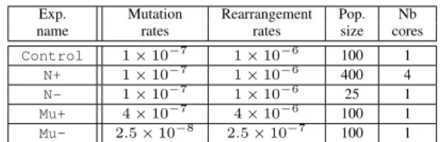
With all these elements in mind, Quentin designed two experiments, one to test the effect of mutation rate and one to test the effect of population size. Following the “in sil-ico experimental evolution” strategy proposed by Batut et al. (2013), evolutionary runs started from a pre-evolved clone (the “Wild-Type”). Here, the same Wild-Type genome was used to seed all evolutionary runs. To test the effect of muta-tion rate, three series of evolumuta-tionary runs were performed: a series of Control runs were performed with the same pa-rameters as those used to produce the Wild-Type, a series of Mu+runs were the mutation rate was increased, and a series of Mu- runs were the mutation rate was increased. For the population size experiment, the same control runs were used as for the mutation rate experiment, and a series of N+ (resp. N-) runs were performed with increased (resp. decreased) population size. All simulations lasted 100,000 generations. Table 1 summarizes the five tested conditions. While de-signing the experiments, we discussed resource allocation. Here the problem was to estimate computation time to es-tablish the number of repeats we were able to compute in a reasonable time. We initially chose to compute five repeats for each condition3. Finally, since in Aevol the computation
time mainly depends on the population size, it was decided to allow more computational resources to the N+ condition.
Tuesday: Preliminary results
The second day of the internship was almost entirely devoted to technical issues regarding Aevol output files, their loca-tion on the disk, how to collect them and the different tools available to analyze them; including the reconstruction of lineages (aevol misc lineage), the computation of lin-eages statistics (aevol misc ancestors stats) and the visualization tools (aevol misc view). For plot-ting and data analysis, we decided to use gnuplot and LibreOffice/Calcas they are user-friendly.
2This was actually the first point we explained to Quentin at the beginning of the internship: we gave him a “notebook” and urged him to write down everything during his internship, including ob-servations, hypotheses, experiments, results or simply ideas.
3All data presented in this paper have been computed with 10 repeats.
Exp. Mutation Rearrangement Pop. Nb name rates rates size cores Control 1× 10⁻⁷ 1× 10⁻⁶ 100 1
N+ 1× 10⁻⁷ 1× 10⁻⁶ 400 4
N- 1× 10⁻⁷ 1× 10⁻⁶ 25 1
Mu+ 4× 10⁻⁷ 4× 10⁻⁶ 100 1
Mu- 2.5× 10⁻⁸ 2.5× 10⁻⁷ 100 1
Table 1: Experimental design. Mutation and rearrangement rates are given in events.bp−1.generation−1. Column “Nb
Cores” corresponds to the degree of parallelism used to com-pute each condition.
From the current state of the simulations, we were able to estimate the total computation time of the experiments and to reevaluate the number of repeats we could do during the internship. We hence decided to add two more repeats in order to increase the statistical accuracy of the results4
Wednesday: Analyzing experimental results
At the beginning of the third day of the internship, all com-putations were finished. We thus entered into a new phase of the scientific method: results analysis. Since Quentin was then autonomous enough with the experiments, we asked him to collect the characteristics of the best organism of each population at generation 100,000 for the five experimental conditions and to compute their mean values. Table 2 shows the corresponding results.
Exp
name Fitness(mean)
Genome length (mean) Coding length (mean) Non-coding length (mean) Wild-Type 0.00632 44,419 bp 12,235 bp 32,184 bp Control 0.00643 44,044.4 bp 12,229.2 bp 31,815.2 bp N+ 0.00766 37,116.9 bp 12,216.4 bp 24,900.5 bp N- 0.00292 46,067.6 bp 11,885.3 bp 34,182.3 bp Mu+ 0.00468 33,693.8 bp 12,003.8 bp 21,690.0 bp Mu- 0.00641 45,226.7 bp 12,166.4 bp 33,060.3 bp
Table 2: Mean characteristics of the best individuals in the populations at generation 100,000 for the five experimental conditions. These values are to be compared with those of the Wild-Type at generation 0 (first row).
Having computed the mean values for these characteris-tics, we entered a decisive step by asking Quentin the fol-lowing question: Can the mean values, as shown in Table 2, be used to draw conclusions about the respective effects of population sizes and mutation rates? In Table 2, all mean values are different – actually means are always different – but part of the difference is due to randomness and sampling
4This decision was not based on the p-values obtained so far since we did not compute them at this stage. Had we decided to add more runs until the p-values became significant, it would have been a form of p-hacking (Head et al., 2015). Note that the experiments presented here are replications of Quentin’s ones and have been performed with a predefined experimental design (with ten repeats per condition).
fluctuations. To clarify this point, we plotted the evolution of genome size along the line of descent of the best final or-ganism for the 100,000 generations of the experiment. We used this temporal data to explain to Quentin that, especially when dealing with stochastic processes, mean values must be used with care as they don’t account for an important el-ement: dispersion. Now, when looking at these graphs, one could have the impression that i) an increased population size leads to genome streamlining (Figure 2) while a reduced population size tends to cause a slight increase in genome size (Figure 3), and that ii) an increased mutation rate leads to genome streamlining while a reduced mutation rate has no effect (figures not shown). Now the decisive question is “is this true?”, opening a discussion about what does being true mean in experimental sciences?
Figure 2: Variation of genome size in the lineage of the clones evolving within an increased population size (N+ clones). Colors indicates the repeats.
Figure 3: Variation of genome size in the lineage of the clones facing a reduced population size (N- clones).
Thursday: Statistical analysis
Having conducted our experiments, it remained to be tested whether the data statistically supported our initial hypothe-ses, namely that both an increase in population size and an increase in mutation rates are likely to cause a genome re-duction.
Given that we had sampled a few evolutionary runs among the infinite number of possible runs, we had only estimates of the mean evolved genome size in each condi-tion. We explained to Quentin that if we were to replicate the experiment, we would sample different runs and hence obtain different mean estimates for each condition. Perhaps this time the observed mean genome size in the N+ condition would not be smaller than the one in the Control condi-tion. In other words, perhaps the smaller genomes we ob-tained in the N+ condition was only due to sampling chance! But we observed a change of mean of more than 15%, is sampling chance alone able to produce that? Actually, yes it is, and not necessarily with a low probability. Thus, we need to quantify the change in mean estimate that is expected by sampling chance only. Regarding the question of scien-tific truth, there is no such thing as experimental truth, only chances of being wrong when drawing conclusions from an experiment...
Given Quentin’s age, it was not possible to enter a de-tailed discussion about random variables, normal distri-butions, statistical inference, parametric or non-parametric tests, etc. We instead decided to go for a semi-statistical, semi-graphical approach, in three steps:
Step 1: the Central-Limit Theorem We first explained to Quentin the basis of the Central Limit Theorem (CLT5).
The CLT tells us that if we replicate many times the pro-cedure of sampling n runs and computing the observed average genome size across the n runs of the sample, and if we draw the histogram of the observed sample means, then we will get a bell shape6. The width of the bell tells
us how much the sample mean is likely to change by sam-pling chance alone, from sample to sample.
Step 2: Confidence Intervals Statistical theory gives us a formula to estimate the width of the bell and to com-pute a so-called Confidence Interval (CI) for the mean. This formula depends both on the observed sample dis-persion and on the sample size. In our case, with n = 10 (i.e. 9 degrees of freedom), the 95% confidence in-terval is CI95% = [¯x ± 2.262p(s2/n)], with s2 =
1 n−1
P(x
i− ¯x) and 2.262 coming from Student’s t
ta-ble for 9 degrees of freedom. A 95% CI captures the true mean for 95% of the samples. We helped Quentin build a spreadsheet to compute s2and the CI95% for each of the
conditions.
5It would have been highly valuable to test it experimentally by e.g. computing more repeats in the Control condition. However, this was impossible in the limited duration of the internship.
6Actually, the random variable X−µ¯
σ/√nhas a standard normal dis-tribution (i.e. normal with expected value 0 and variance 1), and the random variable X−µ¯
s/√n, where s is the Bessel-corrected sam-ple variance, has a Student’s t-distribution with n − 1 degrees of freedom.
Step 3: Do confidence intervals overlap? From confi-dence intervals, we asked Quentin to find a way to identify interesting effects, i.e. those that are most likely not due to sampling chance alone. He decided to check whether confidence intervals overlap or not7. Based on
this criterion, he concluded that “significant” effects were the following:
1. The genome of Mu+ and N+ are smaller than the genome of the Control (Figure 4).
2. The genomes of the Mu+ and N- contain less coding sequences than the genome of the Control and the genome of the N+ (Figure 5, top panel).
3. The non-coding length of Mu+ and N+ are lower than the non-coding length of the Control (Figure 5, bot-tom panel).
Figure 4: Genome size at generation 100,000 for the 5 con-ditions.
Friday: Put the results into perspective
One might think that the previous results, obtained after four days, close the scientific process. We chose to show Quentin that this is not the case, on the contrary! Friday was entirely devoted to discussion between Quentin, his supervisor and the rest of the team. He also presented his results to members of the team who had not followed his work. Our goal was to show Quentin that a scientific result must be put in per-spective and confronted with the current state of knowledge. We also wanted to show him that communicating results and conclusions is an important part of a scientific work: a sci-entist must be able to present his results to the community, discuss them and possibly argue against opponents.
Last but not least for a youngster attracted by a scien-tific career, we discussed the qualities that are necessary to become a researcher, from the obvious (curiosity, rigor, in-tellectual honesty...) to qualities less often put forward but
7Quentin came up with a criterion that is actually used quite often by e.g. biologists, although this approach is not equivalent to performing a statistical test (Krzywinski and Altman, 2013). Here, we performed Kruskall-Wallis tests followed by post-hoc Dunnett tests to compare each condition to the control. We then applied a Bonferroni correction. The p-values of the tests are presented in appendix.
Figure 5: Size of the two main genomic compartments at generation 100,000 for the 5 conditions. Top: coding com-partment. Bottom: non-coding comcom-partment.
just as important: passion, pertinacity, scientific (and non-scientific) culture, or – fundamental for a young French boy – the level of English!
Discussion
During this internship – and in this article – we showed two things. First, that ALife could serve as a powerful pedagog-ical tool to teach the scientific method, including to young and untrained students. Second, that life-traits can strongly influence the length and structure of genomes. Below we separately discuss these two points.
Using ALife to teach the scientific method
Quentin’s internship in the Beagle team illustrated the strength of ALife as a teaching tool. However, contrary to what is generally proposed, here ALife has not been used to teach biology or evolution but rather to teach the scientific method, its main tools and its main issues. We argue that this pedagogical usage of ALife is actually more straight-forward than the former usage. Indeed, using simulation to teach biology requires that the student have preliminary un-derstanding of difficult, abstract and actually fuzzy concepts linked to modelling of biological systems (models being, by essence, different from the system they model). This is even more so for artificial life that intends to model life “as it could be” (i.e. in its whole generality) rather than as it is. It also implicitly implies to change the destination of the models (from mere research to teaching) and its user. Now,
following e.g. Minsky (1965) definition of a model (“To an observer B, an object A∗ is a model of an object A to the extent that B can use A∗to answer questions that interest
him about A”), it is clear that both the observer B and the destination (i.e. the “questions that interest him”) of a model are central in the complex relationship that links the model object A∗to the original object A. In a word, changing the
destination and the user of the model results in such a deep alteration of the A/A∗relationship that it generally implies
changing... the model! This is indeed the process the Avida team engaged through the development of Avida-ED (Speth et al., 2009).
These difficulties vanish when ALife is used to teach the basis of the scientific method, be it during an internship or a labwork. Indeed, in this case, the student is engaged in a scientific process: he/she must answer a question about the model behaviour, exactly as the original user of the model would. Hence there is no change in the model destination and the user change is only minor since the student actu-ally plays the role of a scientist. As a matter of fact, during Quentin’s internship, we did not encounter any conceptual issues regarding the differences between the model and the “real” system. This is simply due to the studied object be-ing Aevol and not what it models. The relationship between the model and the real world was indeed discussed during the internship but that was at the very end (on Friday) and it did not need to be accepted a priori. When Quentin was asked to summarize what he had learned during his intern-ship, his answer was: “During my five day work experience with Inria, I have been able to observe and to learn the re-ality of research and what are the different tasks of this job: to put forward hypotheses, to experiment, to analyze and to publish results. I have learned what are the main qualities of a researcher and what are the studies leading to this job. In only five days, thanks to simulation, I obtained results, I was able to analyze them and then to present them. I noticed that, in teamwork, its very important to have good relations between team members”. Of course, he has also learned a lot about evolution, genomics and genetics. But this appears to be less important that the insights into the scientific process itself...
Of course, we – Quentin and us – encountered difficul-ties during the internship. But most of them were technical, not directly related to the use of Artificial Life. Importantly, none of them proved to be crucial and none compromised the learning process. In fact, the main difficulty encountered was the visualization of the raw data and the visualization of the results of the statistical analyzes. Indeed, all the figures presented in this article were made using R but this software was clearly unusable in the context of such a short educa-tional process. Even though we were able to work around the problem, it would clearly have been desirable to have a simple tool allowing Quentin – a naive user on that matter – to manipulate and visualize the data autonomously.
When teaching the scientific method, ALife proved to have valuable advantages. Here, we will focus on the two main ones. First ALife relies on in silico experiments, which is twice an advantage as it allows for fast experiments that can also be easily replicated (the replication effort being sup-ported by the computer rather than by the student). In the case of Quentin’s internship, a single computer – though a relatively powerful one – was used, enabling him to conduct 5 series of 7 runs, in little more than 24h. Second, using ALife, one can propose internships or labworks focusing on open scientific questions, for which neither the students nor the mentors have a definitive answer. This creates a strong initial motivation and allows to maintain it all along the pro-cess as both the students and the mentors are likely to be surprised – possibly negatively – by the results. In the case of Quentin’s internship, the results shed an interesting light on the process of genome streamlining that deserves to be discussed on its own.
How to reduce a genome?
Genome reduction is common in Nature but its causes are still elusive as biological data suggest that genome reduction could be either neutral or adaptive (Wolf and Koonin, 2013). Our results suggest that at least two distinct mechanisms can lead to genome reduction and that they are distinguishable by their effect on coding sequences. We also show that these mechanisms are triggered by two different causes: increased mutation rates or increased population size.
Interestingly, the effects we observed here fit remark-ably well with what is observed in streamlined bacteria. Indeed, obligate symbionts have an elevated mutation rate (Itoh et al., 2002) while marine cyanobacteria live in very large populations (Batut et al., 2014). Both have under-gone genome streamlining but the reduction is more pro-nounced in obligate symbionts (Figure 1), as in our sim-ulations. Moreover, in these two families, the reduction seemed to have impacted differently the different genomic compartments. Marine cyanobacteria have mainly lost non-coding or duplicated elements, as examplified by Pelagiter ubique, one of the smallest genome of free living bac-teria. Its genome is characterized by a very small fraction of non-coding DNA (less that 5%) and the quasi-absence of redundancy in coding sequences while all metabolic path-ways are still present (Giovannoni et al., 2005). By contrast, the genome of Buchnera aphidicola, an aphid endosymbiont has lost 90% of its genome (compared to E. coli, one of its close relatives), lost several metabolic pathways but, strik-ingly, has conserved 15% of non-coding sequences, a pro-portion similar to what is observed in E. coli (Batut et al., 2013).
The results presented here don’t allow to identify the causal link between mutation rates, population size and genomes size. However, taking advantage of the model char-acteristics – and of our previous results with Aevol, we can
exclude some mechanisms and put others forward. Typi-cally, many authors suggest that genome size may be gov-erned by mutational biases, selection for optimized physio-logical traits (cell size, replication time, energetic costs...) or by transposable elements activities. These are all excluded by our simulation parameters or by Aevol itself. More-over, in Aevol, there is no cost associated to non-coding se-quences. Hence, the influence of population size on genome length cannot be linked to the deleterious effect of non-coding sequences as argued by (Lynch and Conery, 2003).
In the absence of direct selective effects or mutational biases, we hypothesize that genome size is driven by indi-rect selective constraints, namely by selection for robustness (Wilke et al., 2001). Indeed, as already shown by Knibbe et al. (2007), selection for robustness links genome size to mutation rates, the higher the latter, the smaller the former. We hypothesize that the same phenomenon also explains the influence of population size: in large populations, the se-lection strength is higher, increasing the pressure for robust-ness, thereby favouring smaller genomes. The striking ques-tion is then to explain why both phenomena act similarly on non-coding sequences but differently on coding sequences (for which only an elevated mutation rate induces a reduc-tion). We propose that, exactly like selection for fitness, selection for robustness may act positively (selecting more robust clones) or negatively (eliminating clones that are not robust enough – aka purifying selection). Now, in the case of an increased mutation rate, the error threshold (Eigen and Schuster, 1977) moves down and some individuals may find themselves over this crucial threshold. In this case, selec-tion will purify the populaselec-tion from these individuals, re-taining only those that reduced their genome, whatever the elements they have lost (including coding and non-coding sequences). On the opposite, in case of an elevated pop-ulation size, the error threshold does not move down and individuals are still robust enough to maintain their fitness. However, providing adaptive mutations are rare (which is the case here), this results in a positive selection for robust-ness. In this case, individuals must retain their fitness (hence their coding sequences) and the only way to increase their robustness is to get rid of non-coding elements. To the best of our knowledge, these two contrasting effects of selection for robustness had never been identified before. Not content with illustrating the interest of using artificial life to teach the scientific method, our results also show that interesting scientific insights can be gathered meanwhile and open the exciting perspectives of characterizing these two effects in our experiments (by e.g. measuring robustness levels along the evolutionary path), in different conditions and in differ-ent systems.
Material and methods
Simulation platform
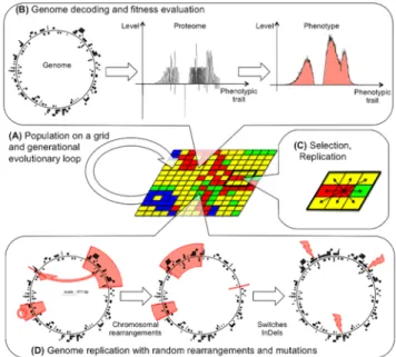
All simulations were run using the regular Aevol model, version 5.0, as available on the platform website (www. aevol.fr). Since Aevol has been extensively described elsewhere (Knibbe et al., 2007; Batut et al., 2013) we will not detail it here and focus only on its core principles and on the elements that are specifically of interest for this paper. Figure 6 shows the main components of the model. Aevol simulates a population engaged in a generational process (Fig. 6.A). Each individual is described by a circular double-strand genomic sequence whose structure closely models a bacterial genome (including non-coding sequences, tran-scription and translation initiation sequences, open-reading frames...) making Aevol an ideally suited platform to study the evolution of genome length and structure. This genome is decoded into a [0 : 1] → [0 : 1] mathematical function which proximity with a target function gives the fitness of the individual (Fig. 6.B). Individuals replicate locally (Fig. 6.C) and, importantly for the present study, Aevol imple-ments a large variety of variation operators (Fig. 6.D) in-cluding mutations (base switches, small insertions and small deletions) and chromosomal rearrangements (duplications, deletions, translocations and inversions). All variation op-erators can be tuned independently, making the platform an ideally suited tool to study indirect selection for mutational robustness.
Figure 6: The Aevol model (figure from (Liard et al., 2018)). (A) Population on a grid and evolutionary loop. (B) Overview of the genotype-to-phenotype map. (C) Local selection process with a Moore neighborhood. (D) Varia-tion operators include chromosomal rearrangements and lo-cal mutations.
Evolution of the Wild-Type strain
To study genome streamlining, we had to give Quentin an initial organism (the “Wild-Type”) that was evolved prior to the internship. In the experiments presented here the wild-type evolved with a population of 100 individuals, a mutation rate of 10−7events.bp−1.generation−1for each of
the three kinds of mutations and a rearrangement rate of 10−6events.bp−1.generation−1for each of the four kinds of
rearrangements. We used an unusually small population size in order to allow for fast experiments.
In order to ensure that the genome size and structure of the wild-type have reached a steady state, we let it evolve for 10 million (107) generations in constant conditions as
preliminary results have shown that the genome size did not stabilize before 5.106 generations (data not shown). Note
that the evolution of genome size and genome structure in the Control conditions (see Table 2) confirmed that the genome was stabilized. We then extracted the genome of the best individual at the last generation. It contains 44,419 bp, 32,184 of which are non-coding and 12,235 coding. It encodes 146 genes transcribed on 108 coding mRNA, ap-proximately half of which being polycistronic. Its fitness is 0.00632. Note that the proportion of non-coding sequences is rather high in this organism, probably because of the small population size.
Experimental design
Starting from the wild-type genome, we used the aevol create tool to initialize a clonal population of wild-types with specific parameters (population size, muta-tion and rearrangement rates, see Table 1). This procedure allowed us to avoid sampling issues when changing the pop-ulation size.
All simulations were then performed on an Intel Xeon CPU with 32-cores at 2 Ghz with 32 Go RAM that Quentin had at his entire disposal for the whole duration of the intern-ship. With this configuration, all the computations required approximately 48h.
Appendix: results of the statistical analyses
Results of the Kruskall-Wallis (KW) and post-hoc Dunnett tests for effects of mutation rates and population size on genome size, coding length and non-coding length. Dun-nett p-values under 0.017 are in bold face (accounting for p<0.05 with a Bonferroni correction for three responses).
Genome size:
KW on mutation rate: χ2= 16.694, df = 2, p-value = 0.0002371 Dunnett: Mu- vs. Control: 0.7205; Mu+vs. Control: 4.4e-06 KW on Population size: χ2= 15.36, df = 2, p-value = 0.000462 Dunnett: N- vs. Control: 0.4661; N+vs. Control: 0.0020 Coding length:
KW on mutation rate: χ2= 13.388, df = 2, p-value = 0.001238 Dunnet: Mu- vs. Control: 0.2833; Mu+vs. Control: 4.9e-05 KW on population size: χ2= 19.311, df = 2, p-value = 6.407e-05 Dunnett: N-vs. Control: 3.5e-07; N+ vs. Control: 0.9523
Non-coding length:
KW on mutation rate: χ2= 16.498, df = 2, p-value = 0.0002615 Dunnett: Mu- vs. Control: 0.6955; Mu+vs. Control: 6e-06 KW on population size: χ2= 15.801, df = 2, p-value = 0.0003705 Dunnett: N- vs. Control: 0.3650; N+vs. Control: 0.0022
References
Batut, B., Knibbe, C., Marais, G., and Daubin, V. (2014). Reduc-tive genome evolution at both ends of the bacterial population size spectrum. Nature Reviews Microbiology, 12(12):841. Batut, B., Parsons, D. P., Fischer, S., Beslon, G., and Knibbe, C.
(2013). In silico experimental evolution: a tool to test evolu-tionary scenarios. BMC bioinformatics, 14(15):S11. Eigen, M. and Schuster, P. (1977). A principle of natural
self-organization. Naturwissenschaften, 64(11):541–565. Giovannoni, S. J., Tripp, H. J., Givan, S., Podar, M., Vergin,
K. L., Baptista, D., Bibbs, L., Eads, J., Richardson, T. H., Noordewier, M., et al. (2005). Genome streamlining in a cosmopolitan oceanic bacterium. science, 309(5738):1242– 1245.
Head, M. L., Holman, L., Lanfear, R., Kahn, A. T., and Jennions, M. D. (2015). The extent and consequences of p-hacking in science. PLOS Biology, 13(3):1–15.
Itoh, T., Martin, W., and Nei, M. (2002). Acceleration of genomic evolution caused by enhanced mutation rate in endocellular symbionts. Proceedings of the National Academy of Sciences, 99(20):12944–12948.
Knibbe, C., Coulon, A., Mazet, O., Fayard, J.-M., and Beslon, G. (2007). A long-term evolutionary pressure on the amount of noncoding dna. Mol. Biol. Evol., 24(10):2344–2353. Krzywinski, M. and Altman, N. (2013). Points of significance:
error bars. Nature methods, 10(10):921.
Liard, V., Parsons, D., Rouzaud-Cornabas, J., and Beslon, G. (2018). The complexity ratchet: Stronger than selection, weaker than robustness. In Artificial Life Conference Pro-ceedings, pages 250–257. MIT Press.
Lynch, M. (2006). Streamlining and simplification of microbial genome architecture. Annu. Rev. Microbiol., 60:327–349. Lynch, M. and Conery, J. S. (2003). The origins of genome
com-plexity. Science, 302(5649):1401–1404.
Minsky, M. (1965). Matter, mind and models. In Proceedings of IFIP Congress, Spartan Books, Wash. DC, pages 45–49. Speth, E. B., Long, T. M., Pennock, R. T., and Ebert-May, D.
(2009). Using avida-ed for teaching and learning about evo-lution in undergraduate introductory biology courses. Evolu-tion: Education and Outreach, 2(3):415.
Wernegreen, J. J. (2002). Genome evolution in bacterial endosym-bionts of insects. Nature Reviews Genetics, 3(11):850. Wilke, C. O., Wang, J. L., Ofria, C., Lenski, R. E., and Adami, C.
(2001). Evolution of digital organisms at high mutation rates leads to survival of the flattest. Nature, 412(6844):331. Wolf, Y. I. and Koonin, E. V. (2013). Genome reduction as the