Centennial-scale elemental and isotopic variability in the tropical and subtropical North Atlantic Ocean

Centennial-Scale Elemental and Isotopic Variability in the

Tropical and Subtropical North Atlantic Ocean

by

Matthew K. Reuer

Bachelor of Arts, Geology

Carleton College, 1995

Submitted in partial fulfillment of the requirements for the degree of

Doctor of Philosophy

at the

MASSACHUSETTS INSTITUTE OF TECHNOLOGY

and the

WOODS HOLE OCEANOGRAPHIC INSTITUTION

February 2002

[JUNE

200]

©

Massachusetts Institute of Technology 2002. All rights reserved.

A uthor .

...

Joint Program in Oceanography/Applied Ocean Science and Engineering

Massachusetts Institute of Technology and Woods Hole Oceanographic Institution

February 15th, 2002

Edward A. Boyle

Professor of Oceanography

Thesis Supervisor

Accepted by ...

A"f

Margaret K. Tivey

Chair, Joint Committee for Chemical Oceanography

Centennial-Scale Elemental and Isotopic Variability in the Tropical and

Subtropical North Atlantic Ocean

by

Matthew K. Reuer

Submitted to the WHOI/MIT Joint Program in Oceanography on February 15th, 2002, in partial fulfillment of the

requirements for the degree of Doctor of Philosophy

Abstract

The marine geochemistry of the North Atlantic Ocean varies on decadal to centennial time scales, a consequence of natural and anthropogenic forcing. Surface corals provide a useful geochemical archive to quantify past mixed layer variability, and this study presents ele-mental and isotopic records from the tropical and subtropical North Atlantic. A consistent method for stable lead isotope analysis via multiple collector ICP-MS is first presented. This method is then applied to western North Atlantic surface corals and seawater, constraining historical elemental and isotopic lead variability. Six stable lead isotope profiles are devel-oped from the western and eastern North Atlantic, demonstrating consistent mixed layer, thermocline, and deep water variability. Finally, coralline trace element records, including cadmium, barium, and lead, are presented from the Cariaco Basin.

First, a reliable method is developed for stable lead isotope analysis by multiple collector ICP-MS. This study presents new observations of the large (0.7% amu 1), time-dependent mass fractionation determined by thallium normalization, including preferential light ion transmission induced by the acceleration potential and nebulizer conditions. These ex-periments show equivalent results for three empirical correction laws, and the previously proposed /Pb/T1 correction does not improve isotope ratio accuracy under these conditions.

External secondary normalization to SRM-981 provides one simple alternative, and a ratio-nale is provided for this correction. With current intensities less than 1.5x10- 12 A, external isotope ratio precision less than 200 ppm is observed (2o). Matrix effects are significant with concomitant calcium in SRM-981 (-280 ppm at 257 piM [Ca]). With the appropriate

corrections and minimal concomitants, MC-ICP-MS can reliably determine 20 6Pb/207Pb and 20 8Pb/207Pb ratios of marine carbonates and seawater.

Anthropogenic lead represents a promising transient oceanographic tracer, and its his-torical isotopic and elemental North Atlantic variability have been documented by proxy reconstructions and seawater observations. Two high-resolution surface coral and seawater time series from the western North Atlantic are presented, demonstrating past variability consistent with upper ocean observations. The elemental reconstruction suggests the pri-mary lead transient was advected to the western North Atlantic from 1955 to 1968, with an inferred maximum lead concentration of 205 pmol kg- 1 in 1971. The mean 1999 North Atlantic seawater concentration (38 pmol kg-1) is equivalent to 1905, several decades prior to the initial consumption of leaded gasoline in the United States. A 20 6Pb/207Pb transient

from 1968 to 1990 is also observed, lagging the elemental transient by ten years. The prove-nance of this isotopic record is distinct from Arctic and European ice core observations and supports a 40% reduction in North American fluxes to this site from 1979-1983 to 1994-1998. Historical isotopic variability agrees with seawater observations, including an isotopic reduction in the western North Atlantic upper thermocline, a consistent 206Pb/20 7Pb ther-mocline maximum in the eastern North Atlantic, and deeper penetration of the elemental lead maximum.

The isotopic composition of anthropogenic lead provides important constraints regarding its time-dependent North Atlantic evolution. The 1998-2001 mixed layer isotopic distribu-tion agrees with zonal atmospheric fluxes between radiogenic westerly and non-radiogenic northeasterly trade wind sources. A non-radiogenic 206Pb/207Pb (1.176) signature in the 1998 western subtropics suggests boundary current advection of equatorial lead, a possi-ble consequence of reduced North American lead fluxes. Isotopic maxima are observed in the mid-latitude thermocline (o0=27) of the eastern and western North Atlantic. This

206_Pb/20 7_{Pb maximum is diminished in both the subpolar and equatorial regions due to}

the prevailing aerosol fluxes, current direction, thermocline ventilation, and lead scaveng-ing. The admixture of Mediterranean Outflow Water reduces the isotopic maximum in the eastern North Atlantic, separable by 206Pb/207Pb and 20 8Pb/20 7Pb ratios. Finally, the deep water variability supports an anthropogenic signature relative to the North Atlantic natural background estimates, with an isotopic range smaller than previously observed. The deep water isotopic composition agrees with the western North Atlantic proxy record and pro-vides a novel chronometric technique: lead ventilation ages of approximately 40 years are observed. Based on its time history, the utility of this tracer is demonstrated by comparing CFC-12 concentrations and 206Pb/20 7Pb ratios in the eastern North Atlantic, including a deep water isotopic boundary between 22 and 31'N.

Finally, the Cariaco Basin is an important archive of past climate variability given its response to inter- and extra-tropical climate forcing and the rapid accumulation of annually-laminated sediments. This study presents annually-resolved surface coral trace element records from Isla Tortuga, Venezuela, located within the upwelling center of this region. The dominant feature of the trace element records is a two-fold Cd/Ca reduction from 1945 to 1955 with no corresponding shift in Ba/Ca, in agreement with the expected hydrographic response to upwelling. Kinetic control of trace element ratios is inferred from Cd/Ca and Ba/Ca results between the coral species S. siderea and M. annularis, consistent with the established Sr/Ca kinetic artifact. Significant anthropogenic variability is also observed by Pb/Ca analysis, observing two maxima since 1920. These potential artifacts cannot com-pletely account for the Cd/Ca transition, supporting a mid-century reduction in upwelling intensity. The trace element records better agree with historical climate records relative to sedimentary faunal abundance records, suggesting a linear response to North Atlantic extratropical forcing cannot account for the observed variability in this region.

Thesis Supervisor: Edward A. Boyle Title: Professor of Oceanography

Acknowledgments

This thesis work greatly benefitted from the generosity, kindness, and diligence of many individuals at the Massachusetts Institute of Technology (MIT), Woods Hole Oceanographic Institution (WHOI), and elsewhere. Without the following people this work would have been impossible, and their efforts will be remembered beyond my limited years in graduate school.

First, several faculty members at MIT and WHOI greatly improved my graduate educa-tion. Lloyd Keigwin supported my initial years in the Joint Program, allowing me to study oceanography and pursue my academic interests. Both Lloyd Keigwin and Tim Eglinton provided encouragement, support, and patience during my first two years at Woods Hole. Several professors also inspired me to pursue geochemistry, notably Bill Jenkins, John Hayes, and Sam Bowring. Finally, John Edmond gave me a world-class introduction to science in general, and his recent passing was a great loss.

An essential aspect of this work was my experience in E34. Rick Kayser provided terrific laboratory and field support, maintaining order in a chaotic lab, finding misplaced tools, and carefully measuring seawater samples. Alla Skorokhod was a great confidant during my five years in E34, and I appreciated her humor, intelligence, and pragmatism. Processing trace element samples is not exactly a typical summer in the United States, and Emmanuelle Puceat provided expert help for the Tortuga record. Finally, Barry Grant was a master teacher of mass spectrometry, computers, machinery, and most technical matters beyond my limited abilities. Whenever disaster struck, the stock answer always was 'Ask Barry'.

Coral samples for this project were generously donated by Julie Cole and Ellen Druffel. Julie fostered my first steps in surface coral research, teaching me many sampling and diving techniques in Venezuela. Her surface coral samples from the Cariaco Basin and the western Pacific allowed development of several useful records and the opportunity to re-established trace element proxies in corals. Ellen Druffel and Sheila Griffin also donated surface coral cores from North Rock, Bermuda, invaluable samples collected nearly two decades ago.

Ed Boyle has provided first-rate scientific resources for this thesis project. Ed's scientific abilities, perseverance, and humor represent the best possible model for a graduate student.

His high personal and scientific standards were inspiring, and I was very fortunate to be his graduate student.

My family and friends have been highly supportive of this academic endeavor. My par-ents, brother, and sister-in-law have been excellent personal role models, and this thesis greatly reflects their support and advice. My friends and fellow students have also kept my sanity intact, with special thanks to Greg Hoke, Kate Jesdale, Juan Botella, Mark Schmitz, Karen Viskupic, and Yu-Han Chen. The students and post-docs of E34 are also thanked for their friendship, help, and advice, including Jess Adkins, Dominik Weiss, Bridget Bergquist, and Jingfeng Wu. Finally, Kalsoum Abbasi provided most of the encouragement and friend-ship needed to finish this project and still laugh at the end of the day.

Biographical Note

Matthew Reuer was born on December 12, 1972 in Rochester, Minnesota. He was raised in Rochester and graduated from John Marshall High School in 1991. In 1995 he received a Bachelor of Arts degree in geology from Carleton College. Upon graduating, the author was employed by the Colorado College from 1995 to 1996, working as a teaching assis-tant in the Department of Geology. In September 1996, he entered the MIT-WHOI Joint Program in Oceanography as a doctoral candidate, specializing in Chemical Oceanography under Edward Boyle. The author is a member of the American Geophysical Union and the Geochemical Society, and is the recipient of a NSF Graduate Research Fellowship, a MIT Presidential Fellowship, and a MIT Graduate Teaching award. Upon graduating from MIT in 2002, he will pursue a post-doctoral fellowship at Princeton University.

Contents

1 Introduction 17

1.1 Cadmium, Barium, and Lead Marine Geochemistry . . . . 18

1.2 Anthropogenic Lead in Seawater . . . . 23

1.3 Lead Isotope Geochemistry . . . . 30

1.4 Coral Biology and Calcification . . . . 33

1.5 Surface Coral Trace Element Geochemistry . . . . 38

1.6 Project O utline . . . . 40

2 Lead Isotope Analysis of Marine Carbonates and Seawater by Multiple Collector ICP-MS 47 2.1 Introduction . . . .. 47

2.2 Methods ... ... 49

2.2.1 Surface Coral and Seawater Sample Preparation . . . . 49

2.2.2 MC-ICP-MS Configuration . . . . 51

2.3 Results and Discussion . . . . 53

2.3.1 Mass Fractionation in MC-ICP-MS . . . . 54

2.3.2 Lead Isotope Ratio Accuracy . . . . 55

2.3.3 Lead Isotope Ratio Precision . . . . 60

2.3.4 Matrix Effects in MC-ICP-MS . . . . 61

2.3.5 Method Assessment and Application . . . . 63

2.4 Conclusions . . . . 66

3 Anthropogenic Lead in the North Atlantic Ocean: Historical Isotopic and Elemental Variability

3.1 Introduction . . . . 3.2 M ethods . . . . 3.3 Results and Discussion . . . . 3.3.1 Western North Atlantic Elemental Lead Records . . . . 3.3.2 Western North Atlantic Lead Isotope Records . . . . 3.4 C onclusions . . . . 3.5 A ppendix I . . . . 4 Stable Lead Isotopes in the Subtro

Ocean

4.1 Introduction . . . . 4.2 M ethods ... . . . ..

4.2.1 Analytical Methodology . . . 4.2.2 Site Hydrography and Climat 4.3 Results and Discussion . . . .

4.3.1 Surface Ocean Variability 4.3.2 Thermocline Variability . 4.3.3 Deep Water Variability . 4.4 Conclusions . . . .

4.5 Appendix I . . . . 5 Centennial-Scale Tropical Upwelling

Trace Element Proxies

5.1 Introduction . . . . 5.2 M ethods . . . .

5.2.1 Analytical Methodology . . .

5.2.2 Cariaco Basin Hydrography .

pical and Tropical North Atlantic 89 . . . . 90 . . . . 9 2 . . . . 9 2 )logy . . . . 95 . . . . 9 5 . . . . 10 1 . . . . 10 7 . . . . 111 . . . - . . . .. 114 . . . - 117 Variability Inferred from Coralline

119 120 122 123 125 125 127 5.2.3 Tropical North Atlantic Climatology

5.3 Results and Discussion . . . .

.

5.3.1 Surface Coral Trace Element Artifacts . . . . 5.3.2 Seasonal Trace Element Variability . . . . 5.3.3 Decadal-Scale Trace Element Variability . . . . 5.3.4 Interdecadal Trace Element Variability . . . . 5.4 Conclusions . . . . A Surface Coral Preparation and Elemental Analysis

A.1 Acquisition and Sampling . . . . A.2 Sam ple Cleaning . . . . A.3 GFAAS Analysis . . . . A.4 Isotope Dilution ICP-MS . . . . A.5 M ethod Validation . . . . B North Rock Surface Coral Pb/Ca and Lead Isotope Results

B.1 North Rock Pb/Ca Results . . . . B.2 North Rock and Station S Stable Lead Isotope Results . . . . .

128 134 135 138 142 153 153 155 157 158 159 163 164 167

List of Figures

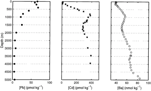
1-1 Water column profiles for cadmium, barium and lead . . . . 1-2 Global background and anthropogenic heavy metal emissions . . . . 1-3 Historical global lead production since 5000

1

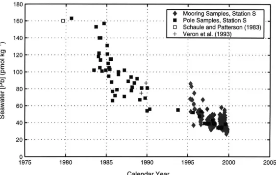
1-4 Historical leaded gasoline consumption, United States and western Europe . 1-5 Station S, Bermuda seawater lead time series analysis, 1979-2000 . . . . 1-6 1-7 1-8 1-9 1-10 1-11 1-12 2-1 2-2 2-3 2-4 2-5 2-6 2-7 2-8 2-9

North Atlantic thermocline lead evolution . . . . 29

Triple isotope diagram for primary lead ores and coal . . . . 32

Surface coral structure and calcification . . . .. . . . . 34

Global coral reef distribution. . . . . 35

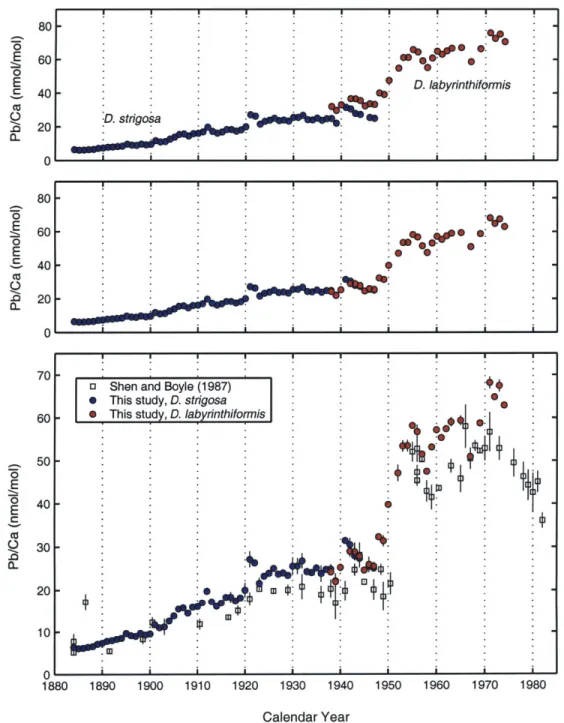
North Rock, Bermuda Pb/Ca record of Shen and Boyle (1987) . . . . 41

Galapagos Islands Ba/Ca record of Lea et al. (1989).... . . . . 42

Element-calcium ratios for surface corals and seawater . . . . 44

IsoProbe MC-ICP-MS schematic . . . . 52

IsoProbe mass fractionation experiments . . . . 56

Empirical mass fractionation models for MC-ICP-MS . . . . 57

Log transforms of 207Pb/206Pb, 208Pb/206Pb, and 20 5T1/ 203T1

. . . .

SRM-981 external precision experiments . . . . 62

IsoProbe calcium matrix experiments, SRM-981 . . . . 64

Western North Atlantic surface coral proxy record and seawater time series 67 Eastern North Atlantic stable lead isotope and concentration profiles . . . . 68

3-1 North Rock surface coral Pb/Ca records, Diploria sp. . . . . 76

3-2 Western North Atlantic lead reconstruction... . . . . . . . 78

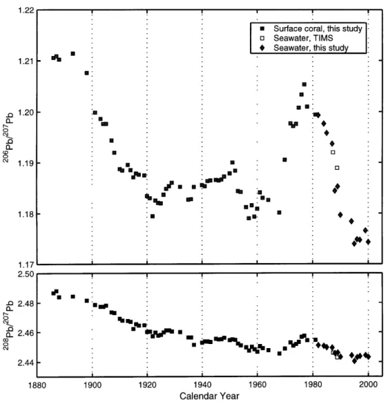
3-3 Western North Atlantic lead isotope reconstruction . . . . 80

3-4 Lead isotope proxy record comparison, 206Pb/207Pb . . . . 82

3-5 Triple isotope diagram, North Atlantic, Greenland, and European records . 83 3-6 Western North Atlantic thermocline 20 6Pb/20 7_{Pb evolution . . . . 85}

3-7 Eastern North Atlantic lead isotope and concentration profiles . . . . 86

4-1 North Atlantic 206Pb/207Pb distribution, 1987-1989 . . . . 91

4-2 North Atlantic site location map and mean annual SST distribution . . . . 93

4-3 North Atlantic seasonal mixed layer depth, density, and wind speed vectors 96 4-4

0-S

4-5 Lead isotope profiles, eastern and western North Atlantic, 1998-2001 . . . . 102

4-6 Lead concentration profiles, eastern and western North Atlantic, 1998-2001 103 4-7 North Atlantic surface ocean lead isotope results . . . . 104

4-8 North Atlantic surface ocean lead isotope comparison . . . . 106

4-9 o- 206Pb/207Pb plot, eastern and western North Atlantic . . . . 109

4-10 Thermocline elemental and stable isotope comparison, Stations 7 and 4 . . 110

4-11 North Atlantic deep water isotopic variability . . . . 112

4-12 CFC-12 and lead isotope comparison, eastern North Atlantic . . . . 116

4-13 Spherical distances between two points on a planar trapezoid . . . . 117

4-14 Particle trajectory approximation, western North Atlantic Station 1 . . . . 118

5-1 Dissolved cadmium and barium profiles from the Cariaco Basin . . . . 122

5-2 Surface coral X-radiograph positives, M. annularis and S. siderea . . . . 124

5-3 Cariaco Basin site location map and winter SST distribution . . . . 126

5-4 Isla Tortuga raw Cd/Ca and Ba/Ca records . . . . 129

5-5 Isla Tortuga Cd/Ca and Ba/Ca annual means . . . . 130

5-6 Isla Tortuga Cd/Ca and Ba/Ca annual amplitude . . . . 131

5-7 Trace element interspecies comparison, S. siderea and M. annularis . . . . . 133

5-9 Trace element seasonality, Cariaco Basin . . . . 136

5-10 Spectral analyses, Cd/Ca and faunal abundance records . . . . 137

5-11 Historical climate records from the Cariaco Basin . . . . 139

5-12 Cariaco Basin proxy records and historical climate comparison . . . . 140

5-13 Correlation map of Cariaco Basin historical SST . . . . 142

A-1 Protocol for surface coral sample preparation and analysis . . . . 154

List of Tables

1.1 Surface coral cation compilation . . . . 1.2 Surface coral Cd/Ca ratios and mean annual phosphate comparison . . . .

2.1 IsoProbe MC-ICP-MS instrumental conditions . . . . 2.2 Procedural blank analysis, MC-ICP-MS . . . . 2.3 SRM-981 mass fractionation experiment . . . . 2.4 SRM-981 isotope ratio accuracy experiment . . . .

2.5 SRM-981 compilation, TIMS and MC-ICP-MS . . . .

3.1 Lead provenance estimates for the western North Atlantic . . . . . 4.1 Hydrographic stations, eastern and western North Atlantic . . . . 4.2 North Atlantic lead isotope results, 1998 to 2001 . . . . 4.3 Lead concentration results, eastern and western North Atlantic. . . 5.1 Cd/Ca and Ba/Ca results, Isla Tortuga, Cariaco Basin . . . . A.1 Standard GFAAS temperature program . . . . A.2 VG PlasmaQuad 2+ quadrupole ICP-MS instrumental conditions . B.1 Pb/Ca results: North Rock, Bermuda . . . . B.2 Lead isotope results: North Rock, Bermuda . . . .

. . . . . 50 . . . . . 53 . . . . . 60 . . . . . 60 . . . . . 65 . . . . . 81 . . . . . 94 . . . . . 98 . . . . . 100 144 157 160 . . . . . 164 . . . . . 167

Chapter 1

Introduction

The trace element geochemistry of the world oceans is directly associated with multiple global-scale phenomena, including the global carbon cycle, the land-air-sea mass balance, and anthropogenic heavy metal emissions. Despite their established importance, limited time series observations presently exist, with most seawater observations spanning the past two decades from a few locations (Wu and Boyle, 1997a). To address this issue, surface corals offer an important archive to constrain past geochemical variations in the tropical and subtropical surface ocean at seasonal resolution. This thesis project utilizes this approach to (1) examine past tropical upwelling variability in the Cariaco Basin, Venezuela; (2) quantify the flux and provenance of anthropogenic lead in the western North Atlantic; and (3) compare the reconstructed lead variability with recent hydrographic observations from the eastern and western North Atlantic. These centennial-scale records demonstrate the non-steady state, time-dependent distribution of multiple trace elements in the tropical and subtropical surface ocean, resulting from both natural and anthropogenic forcing.

The utility of carbonate geochemical proxies has three prerequisites: a quantitative understanding of modern elemental distributions, a carbonate host faithfully recording sea-water chemistry, and an isolatable signal of adequate magnitude. Marine trace element variability has been well-established (e.g., Boyle et al., 1976; Chan et al., 1977; Boyle et al.,

1981; Bruland and Franks, 1983; Schaule and Patterson, 1983; Johnson et al., 1997), quan-tifying the relative importance of biological cycling, atmospheric deposition, and ocean circulation on trace element geochemistry. Trace element proxies in marine carbonates

was first systematically established for Cd/Ca ratios in benthic foraminifera, including synchronous glacial-interglacial Cd/Ca and

6

in North Atlantic Deep Water formation (Boyle and Keigwin, 1982, 1987; Boyle, 1988). Finally, adequate surface ocean trace element variability is expected given a six-fold dif-ference in cadmium concentrations across the equatorial Pacific (Boyle and Huested, 1983) and a two-hundred fold difference in anthropogenic lead fluxes observed in Arctic ice cores (Murozumi et al., 1969; Boutron et al., 1991; Candelone et al., 1995).

Surface corals offer a promising, seasonally-resolved trace element archive, demonstrated by several previous studies (e.g., Shen et al., 1987; Lea et al., 1989; Shen et al., 1992a). Trace elements and their isotopes provide independent evidence for past variations in upwelling intensity, fluvial influxes, nutrient status, and anthropogenic fluxes in the tropical and sub-tropical surface ocean. These results provide new geochemical observations and test the underlying assumptions of the established coral proxies, including minor element ratios (Sr/Ca, Mg/Ca), stable isotopes (6180, 613C), and radiogenic isotopes (Al4_C, 2 10_{Pb, see}

reviews by Dunbar and Cole, 1993; Druffel, 1997; Gagan et al., 2000). Trace element mea-surements can incorporate several elemental and isotopic proxies from an individual sample (e.g., Cd, Ba, Pb, Zn, V, and Fe), although most of these systems are largely unexplored. The annual density couplets and rapid extension rates of surface corals, coupled with ra-diometric age-dating techniques (Edwards et al., 1987), provide a continuous, independent, and high-resolution chronology.

1.1

Cadmium, Barium, and Lead Marine Geochemistry

The first consideration for trace element proxies is their modern hydrographic distribution. Given their low seawater concentrations relative to the major cations (e.g., 49.7 pmol kg-1 for North Atlantic mean 1996 total lead concentration, Wu and Boyle, 1997a), trace element analyses prior to 1976 were frequently compromised by sampling and analytical contam-ination. The difficulty of trace element analyses is both minimizing and quantifying the blank contribution for each step of the sampling and analytical protocol (see Tables 1 and 2 of Patterson and Settle, 1976), frequently testing methods, materials, and reagents. For

500 1000 1500 2000 E =6_ 2500 3000 3500 4000 4500 5000 0 -- --- - -.-- - - - --- -.- - - - -... 0 50 100 [Pb] (pmol kg-') -- - -u Emir ... . . . . . . 0 200 400 [Cd] (pmol kg-') 0

Figure 1-1: Water column profiles for cadmium, barium, and lead. The lead seawater profile, from Schaule and Patterson (1983, central northeast Pacific, 32'41'N, 145'00'W), exhibits clear particle-scavenging effects, with reduced concentrations from mixed layer to interme-diate depths. The cadmium profile, from Wu and Boyle (1997b, eastern North Atlantic, 26025'N, 33'40'W), shows a nutrient-like profile from biological uptake and remineraliza-tion. The barium profile demonstrates deeper barium regeneration from biogenic barite dissolution (Chan et al., 1977). The secondary [Ba] maximum at 900 meters also reflects Antarctic Intermediate Water in the western North Atlantic.

seawater this challenge was addressed by several independent studies (Boyle and Edmond, 1976; Boyle et al., 1976; Martin et al., 1976; Bruland et al., 1978; Schaule and Patter-son, 1983), demonstrating consistent water column profiles among the major ocean basins (Figure 1-1). Here the generalized marine geochemistry of cadmium, barium, and lead is presented, demonstrating the relative importance of biological cycling, particle scavenging, and hydrography on their recent water column distribution.

Oceanic Cadmium Variability

The marine cadmium cycle is dominated by biological uptake and remineralization, resulting in a nutrient-type distribution similar to nitrate and phosphate. Boyle et al. (1976) first

19 0-- - - . . - - . . -.0 0... . 0 0 0 0 0 0 0 0. 0 40 60 80 100 [Ba] (nmol kg-')

demonstrated the correlation between seawater cadmium and phosphate concentrations in the Pacific, with water column Cd/P ratios (0.4 mmol/mol) consistent with plankton Cd/P ratios (0.4 to 0.7 mmol/mol). Water column profiles showed higher correlation with phosphate compared to silicate, suggesting cadmium regeneration from labile, organic-rich phytoplankton remains. Mechanistically, it has been suggested that part of the cadmium-phosphorus association results from carbonic anhydrase activity in marine phytoplankton (linked to zinc-carbonic anhydrase activity, Lee and Morel, 1995), and a distinct cadmium-carbonic anhydrase has been observed by Cullen et al. (1999). Direct correlation between cadmium, nitrate, and phosphate is complicated, however, by preferential trace element uptake relative to the major nutrients (see Figure 12 of Boyle et al., 1981) and possible pCO₂ effects (Cullen et al., 1999), resulting in multiple Cd/P relationships in the world oceans (Elderfield and Rickaby, 2000). Despite these complications, the nutrient-like distribution is demonstrated by cadmium accumulation within water masses; the North Atlantic deep water concentration (0.3 nmol kg-1, Bruland and Franks, 1983) is approximately three-fold lower than the deep Pacific (1.0 nmol kg-1, Bruland, 1980), consistent with diminished A14C in the deep Pacific (see Figure 5-4 in Broecker and Peng, 1982). A large surface water cadmium concentration gradient (ca. 15 to 85 pmol kg- 1) across the eastern equatorial Pacific upwelling zone has also been observed by Boyle and Huested (1983), supporting its promise as an upwelling indicator. Thus cadmium geochemistry largely reflects major nutrient cycles and their hydrographic distribution.

The speciation of dissolved' cadmium in seawater is dominated by organic ligands and chloride complexes. As shown by Bruland (1992), 70% of dissolved cadmium in the central North Pacific mixed layer is bound to strong organic ligands, present at low concentrations (Keond = 1012 M-1, [L]<0.1 nM). This ligand was not observed below 175 meters, suggesting inorganic cadmium complexes are the primary species below the euphotic zone. Under standard conditions (pH 8.1, 25'C, 1 atm), cadmium chloride complexes are the principal species, including CdCl' (51%), CdCl+ (39%), and CdCl3 (6%, Zirino and Yamamoto, 1972). Free Cd2+ accounts for 2.5% of the dissolved inorganic fraction; other secondary

'Here 'dissolved' is operationally defined, reflecting all cadmium passing through a 0.45 pLm filter and including colloidal and soluble phases.

species (CdSO', CdOH+, CdHCO+, and CdCO') are present below 1%.

The recent global cadmium cycle has been greatly altered by anthropogenic emis-sions. Background global cadmium emission estimates equal 1.3x109 _{g yr-} 1 _{(Nriagu, 1989),}

whereas anthropogenic emissions reached 7.6x109 _{g yr} 1 _{in 1983, derived primarily from} copper-nickel smelting, coal combustion, and steel manufacture (Nriagu and Pacyna, 1988). From surface coral Cd/Ca measurements from 1865 to 1982, Shen et al. (1987) inferred a five-fold increase in cadmium concentrations (0.26 to 1.37 nmol/mol) in the western North Atlantic surface ocean. The corresponding deep water response, however, should be minimal. For example, with an assumed area (4.1x107 _km2_{), depth (3800 meters), and}

cadmium concentration below 1000 meters (334 pM), the North Atlantic cadmium inven-tory equals 7.9x1012 g. If all the global cadmium emissions were deposited in the North Atlantic (7.6x109 g yr- 1) with no loss to particle scavenging, approximately one thousand years would be required to double the inventory. The biological uptake, regeneration, and advection of cadmium in the deep North Atlantic thus results in a heterogenous response to anthropogenic forcing.

Marine Barium Geochemistry

Barium geochemistry reflects the formation and regeneration of biogenic barite and the sub-sequent hydrographic distribution of dissolved barium, resulting in water column profiles similar to dissolved silica and alkalinity (Wolgemuth and Broecker, 1970; Chan et al., 1977; Dehairs et al., 1980; Collier and Edmond, 1984; Lea and Boyle, 1989). Upper ocean barium concentration gradients result from biogenic barite cycling, ranging from approximately 70 nmol kg- 1 in the surface mixed layer to 100 nmol kg-1 _{at 2000 meters (Antarctic}

Circumpo-lar Current, Chan et al., 1977). Bishop (1988) first observed the association among barite, opal, and organic carbon in marine particulate matter (>53 pm), noting high barium con-centrations associated with siliceous diatom and dinoflagellate remains. The dissolution of these biogenic phases in marine sediments represents a significant barium source over high productivity regions: McManus et al. (1994) calculated a benthic barium flux of 25 to 50 nmol cm 2 yr~1 from the California continental margin. Second, hydrographic variability affects barium concentrations in the world oceans. For example, Chan et al. (1977) observed

barium concentration maxima in Antarctic Intermediate Water and Antarctic Bottom Wa-ter in the wesWa-tern North Atlantic, similar to the established silica distribution. Correlations among [Ba], [Si], and alkalinity should not be overstated, however, given their different sources in high-latitude regions (see Figure 16 of Chan et al., 1977). Despite these compli-cations, the marine barium cycle reflects barite formation in siliceous microenvironments, barium regeneration in seawater and marine sediments, and its subsequent hydrographic distribution.

In contrast to cadmium and lead, limited barium species are observed in seawater. Under standard conditions, Byrne et al. (1988) calculated 96% of dissolved barium exists as free Ba2+, with only 4% present as BaSO'. No association with organic ligands in seawater has been demonstrated.

Lead Geochemistry

The marine geochemistry of lead is dominated by aeolian deposition and scavenging, with no biological lead utilization. The importance of aeolian deposition was demonstrated by Schaule and Patterson (1981) for the central North Pacific, observing increased lead con-centrations and 2 10Pb activity from coastal western North America (Monterey Bay) to the subtropical North Pacific gyre (Hawaii), consistent with the spatial distribution of North Pacific 2 1 0_{Pb (Nozaki et al., 1976). The atmospheric transport pathway is also supported by} vertical profiles in North Atlantic and Pacific, with low deep (26 pmol kg- 1_{, 2980 meters)}

and thermocline (77 pmol kg-1, 1000 meters) lead concentrations in the Sargasso Sea rela-tive to the surface mixed layer (160 pmol kg-1, 0.5 meters). Scavenging and regeneration of aerosol-derived lead results in short residence times relative to cadmium and barium. From

2 2 6_Ra-2 10

Pb disequilibria (Craig et al., 1973; Bacon et al., 1976; Nozaki and Tsunogai, 1976), the lead residence time ranges from two years for the surface mixed layer to several decades for the upper thermocline. For example, Bacon et al. (1976) estimated integrated lead residence times of 20 to 93 years for six stations in the equatorial Atlantic over the depth range 451 to 5003 meters. Finally, mixed layer and upper thermocline lead also exhibits strong seasonality, demonstrated by Boyle et al. (1986) in the western North Atlantic. This seasonality reflects winter mixed layer depths reaching 200 meters, spring scavenging due to

elevated biological productivity, and summer accumulation within a stratified mixed layer. Thus the marine lead cycle reflects atmospheric inputs, seasonal upper-ocean variability, and particulate scavenging and regeneration.

The predominant atmospheric pathway warrants consideration. Recent atmospheric lead is associated with sub-micron, carbonaceous aerosols derived from high-temperature, anthropogenic sources (Rosman et al., 1990), with a tropospheric residence time of 9.6±2.0 days (Francis et al., 1970). _{As shown by the XRD analyses of Biggins and Harrison} (1979), the composition of anthropogenic lead aerosols includes halogens derived from au-tomobile exhaust (PbBrCl, PbBrCl-2NH4Cl, and a-2PbBrCl.NH4Cl) and sulfates (PbSO4,

PbSO4-(NH4)2SO4). Wet deposition dominates lead removal from the atmosphere,

account-ing for approximately 85% of the total deposition (see Duce et al., 1991, and refs. therein). Solubility estimates of particulate-adsorbed lead are presently uncertain, ranging from 13 to 90% (Hodge et al., 1978; Maring and Duce, 1990). Thus lead is effectively transported by and removed from the troposphere to the surface mixed layer.

Dissolved lead accounts for approximately 90% of the total lead concentration in olig-otrophic gyres (Shen and Boyle, 1987), and a significant fraction of the dissolved phase might be complexed with organic ligands. For example, Capodaglio et al. (1990) observed 50 to 70% of dissolved lead is complexed with a strong organic ligand in the eastern North Pacific (Ke'fl = 109.7 M 1); no North Atlantic measurements presently exist. The re-maining dissolved phase is dominated by inorganic complexes: Whitfield and Turner (1980) calculated from equilibrium models that PbCO' accounts for 55% of the dissolved inorganic fraction, followed by PbCl' (11%), Pb(C0 3,Cl3)~ (10%), and PbCl+ (7%). The remaining

17% includes chloride (PbCl3, PbCl2-), sulfate (PbSO'), and hydroxide (PbOH+) species, with free Pb2+ comprising less than 2% of total dissolved inorganic lead.

1.2

Anthropogenic Lead in Seawater

Of all heavy metals in the environment, global lead emissions have been most affected by human activities. The emission inventory method of Nriagu and Pacyna (1988) suggests 97% of modern lead fluxes are anthropogenic, and the global annual emissions for five

met-x108 4-en 0 3 A0 E .2 2 (D 0.

4-<0

_{FJ F}

n n

I

Figure 1-2: Global background and anthropogenic heavy metal emissions for cadmium, copper, nickel, zinc, and lead. The white bars reflect the background estimates of Nriagu (1989), the black bars denote the Nriagu (1979a) anthropogenic estimates for 1975, and the gray bars represent the Nriagu (1989) anthropogenic estimates for 1983. Note the predominance of zinc and lead relative to the other heavy metals, with the anthropogenic component from 56% for Cu to 97% for Pb in 1983.

als are shown in Figure 1-2. The median global lead emission for 1983 equals 3.3x1011 _g

yr-1 , thirty-fold higher than the natural background (1.2x1010 g yr-1 Nriagu, 1989). Nat-ural lead sources include soil dusts (3.0x109 _{g yr-}1_{), volcanic emissions (3.3x10}9 _{g yr--),}

forest fires (1.9x109 g yr-1), seasalt aerosols (1.4x109 g yr-1), and continental particulate matter (1.3x109 g yr- 1, Nriagu, 1989). As shown in Figure 1-3, adapted from Settle and Patterson (1980), anthropogenic lead production has occurred since approximately 5000 1C years before present, associated with the discovery of cupellation2. Modern anthro-pogenic emissions, however, are dominated by leaded gasoline consumption, accounting for approximately 75% of the total emissions in 1983. Historical variations in leaded gasoline consumption is shown in Figure 1-4, including consumption patterns in the United States and western Europe from 1930 to 1990. The smelting of non-ferrous metals (including

pri-2

Cupellation is the separation of gold or silver from argentiferous lead, refining the ore in a porous furnace (a cupel). The impurity metals (e.g., Pb, Cu, and Sn) are oxidized, vaporized, and partly adsorbed onto the porous cupel during blast heating. This fire assay and refining technique is considered the oldest quantitative chemical method; a thorough historical and technical review is given by Nriagu (1985).

mary lead, copper-nickel, and zinc-cadmium), accounts for the remaining 25%, although this contribution is currently increasing with the progressive phaseout of leaded gasoline from North America and western Europe (Wu and Boyle, 1997a).

Three properties of modern lead aerosols provide independent evidence of their primary anthropogenic origin. First, the elevated Pb/Ba ratio of pristine soils support its anthro-pogenic origin (Patterson and Settle, 1987). This technique normalizes lead concentrations with respect to barium, determining the natural Pb/Ba ratio from the High Sierra source quartz monzonite and a minor (Baseasat/Badust=0.07) seasalt correction to the aerosol Ba (Patterson and Settle, 1987). Using this method, Patterson and Settle (1987) estimated industrial lead accounted for 88% of total lead concentrations in High Sierra soil humus and litter. Measured aerosol lead concentrations are also approximately ten-fold smaller on air filters relative to precipitation at the same location, a consequence of high-temperature an-thropogenic sources enriching the sub-micron, halogenated, and carbonaceous mode readily scavenged by wet deposition (Ng and Patterson, 1981; Patterson and Settle, 1981). Second, the aerosol lead fluxes across the central Pacific are greater in the Northern Hemisphere, ranging from 0.02 ng cm- 2 yr- 1 for the south polar cell to 50 ng cm-2 yr-1 in the North Pa-cific westerlies (Patterson and Settle, 1987, and refs. therein). An Atlantic-PaPa-cific difference is also observed for the Northern Hemisphere, with 170 ng cm-2 yr-4 measured from the North Atlantic westerlies (ibid.). Finally, mass balance calculations support predominant anthropogenic fluxes. Assuming a two-year residence time in the upper 100 meters and a lead concentration of 160 pmol kg-1 (Schaule and Patterson, 1983), the resulting lead flux is 175 ng cm-2 yr 1. This estimate is approximately six times greater than the maximum natural output flux of 30 ng cm-2 yr-1 calculated from the accumulation and lead con-centration of pelagic sediments (Chow and Patterson, 1962). The difference between this anthropogenic to background ratio (5.8) and the Nriagu (1989) estimate shown in Figure 1-2 (27.7) most likely results from the spatial scales between global (Nriagu, 1989) and North Atlantic estimates; uncertainties in the lead residence time and possible seasonal aliasing of the Schaule and Patterson (1983) observation will also contribute to this difference.

The observed anthropogenic fluxes have corresponding seawater signatures. First, Wu and Boyle (1997b) observed a three fold reduction in seawater lead concentrations near

IU |

106

Industrial

.0 10 Roman Republic .4 Revolution

--and Empire 0 0 10- Spanish Ag

2-

7German

Corrected Radiocarbon Age (yBP)

Figure 1-3: Historical global lead production since 5000 14C years before present, adapted from Settle and Patterson (1980). The derivation of this curve is based on the lead content of cerargyrite (AgCl), global silver production, and historical lead production data (see footnotes in Settle and Patterson, 1980). Note the ordinate is shown on a logarithmic scale.

300 250 C S00 50 0 CL 0 00 0 1930 1940 1950 1960 1970 1980 1990 Calendar Year

Figure 1-4: Historical leaded gasoline consumption, United States and western Europe. The figure and the associated data are taken from Wu and Boyle (1997a) and references therein. The nations shown include the United States (USA), France (FR), Italy (I), the United Kingdom (GB), and Germany (D). The maximum leaded gasoline consumption in the United States occurred in 1972, corresponding to 84% consumption with respect to the nations shown here.

Bermuda, from 160 pmol kg-1 (Schaule and Patterson, 1983) in 1979 to 49.7 pmol kg 1 in 1996 (Figure 1-5). This apparent reduction includes a large seasonal cycle due to the lead mixing-scavenging-accumulation cycle (see above and Boyle et al., 1986). The three-fold reduction in seawater lead concentrations is concurrent with known reductions in leaded gasoline consumption in the United States from 1979 to 1993 (190x103 to 10x103 metric tons yr- 1), providing a direct link between US lead emissions and seawater lead concentrations. Second, vertical lead concentration profiles provide additional evidence for reduced anthro-pogenic lead fluxes. Because the western North Atlantic upper thermocline is ventilated on decadal timescales (from 3H_3He measurements of Jenkins, 1980), a comparable reduction in thermocline lead concentrations should be observed. As shown in Figure 1-6, vertical profiles from 1979 (Schaule and Patterson, 1983) to 1998 (E. A. Boyle, unpublished results) exhibit a consistent reduction to approximately 1000 meters. The shape of the elemental

I I I I - - . - - - -.- : - - - : -.. : . :. U *+ U -+ -. --. .--. --. . --. . .-. .-. .- -.. --... .. .. .. .... ..+.. . - - - --- - - --- - - ---. -1985 1990

* Mooring Samples, Station S * Pole Samples, Station S

-o Schaule and Patterson (1983)

+ Veron et al. (1993)

..----

--

--.

-

---.

_-

4

Figure 1-5: Bermuda seawater lead time series analysis, 1979-2000, adapted from Wu and Boyle (1997a). Surface mixed layer lead concentrations (in pmol kg') from Station S are shown, including results from Schaule and Patterson (1983, 0) and V6ron et al. (1993, +). The closed squares were collected by the pole sampling method at Station S, and closed diamonds reflect MITESS mooring samples. See Wu and Boyle (1997a) for additional details.

profiles are clearly different, due to the declining mixed layer concentrations concurrent with reduced anthropogenic emissions, the increasing ventilation time scales with depth in the western North Atlantic (Jenkins, 1980), the seasonality of lead scavenging, regenera-tion, and accumulation within the upper 200 meters (Boyle et al., 1986), and sampling or analytical artifacts. Both the western North Atlantic mixed layer and the thermocline lead concentrations have declined according to the anthropogenic lead transient.

Terrestrial and marine proxy data provide additional constraints regarding the anthro-pogenic transient. Measuring lead concentrations in ice near Camp Century, Greenland, Murozumi et al. (1969) first observed the Arctic anthropogenic transient, with lead concen-trations increasing from less than 0.001 pg g- 1 at 800 BC to greater than 0.200 pg g- 1 in 1965. The greatest increase in lead concentration occurred after 1940, in agreement with Eurasian and North American leaded gasoline consumption patterns. A ten-fold

concentra-160 ... 140 ... 120 ... 100 ... 80 ... 60 ... A . ... 201-... 0-1975 1980 2005

0 El 100 * . -- S e 1979 1998 -200 1993 1989 '+ 300-- _{300 4 *1984} - + e 400 C 500 .c 500 * . 00 80 600 - .* 0 : 700 -800 0 900 0 1000 --

Figure 1-6: North Atlantic thermocline lead evolution: 1979 to 1998. Six profiles are shown from the western North Atlantic: Schaule and Patterson (1983, E, collected 1979), Boyle et al. (1986, o, collected 1984), V6ron et al. (1993, +, collected 1989), Wu and Boyle (1997a, *, collected 1993), and unpublished results of E. A. Boyle [+, collected 1998]. The 1984 profile represents the mean of three profiles taken in April, June, and September (Boyle

et al., 1986).

tion difference between 800 BC (<0.001 pag g- 1) and 1750 AD (0.011 Ag g- 1) also suggests significant anthropogenic lead fluxes prior to the Industrial Revolution, in agreement with Figure 1-3. Other terrestrial records, including peat cores and lacustrine sediments, pro-vide useful constraints on past anthropogenic variability (e.g., Shirahata et al., 1980; Ritson et al., 1994; Graney et al., 1995; Shotyk et al., 1998; Weiss et al., 1999). From a Jura Moun-tain peat core, Shotyk et al. (1998) observed a significant increase in Pb/Sc ratios at 3000 14C _{yr. BP, indicating the first European anthropogenic lead signatures associated with}

Phoenician and Greek lead mining. The recent transient at the Jura Mountain site (15.7 mg m-2

yr-1, 1979) was also 1570 times the natural background value (0.01 mg m-2 _yr-),

significantly higher than the Greenland natural to anthropogenic ratio. Finally, surface coral records (Shen and Boyle, 1987) and marine sediments (Ng and Patteron, 1982; Veron et al., 1987) provide additional constraints on anthropogenic fluxes to the world oceans. Measuring the Pb/Ca ratio of surface corals from Bermuda and the Florida Straits, Shen and Boyle (1987) estimated an eleven-fold increase in anthropogenic lead fluxes to the west-ern North Atlantic from 1884 (5.2 nmol/mol) to 1971 (56.7 nmol/mol). Proxy records provide independent evidence for global-scale, time-dependent anthropogenic lead fluxes to terrestrial and marine environments.

1.3

Lead Isotope Geochemistry

The isotopic composition of recent lead represents an established, independent atmospheric and oceanic tracer. Lead isotope fractionation is governed by the age and initial U-Th-Pb content of an ore body. Radiogenic ingrowth of 2 0 8_{Pb from} 232_Th, 20 7_{Pb from} 23 5_{U, and} 206

_Pb

U can be written as:

206

_Pb

_Pbo

_Pb

_{Pbo +}

_EeA235to

-

eA235t

(1.2)

208 = 2 0 8 Pb + 2 3 2Th - eA232to - eA232t (1.3)

where the subscript [o] reflects the primeval isotopic abundance, to denotes the age of the Earth, t is the emplacement age, and A, represents the half lives for 238_{U (1.55125x10-}10

y-') 2 3 5_{U (9.8485x10-} 10 _y-1_{), and} 2 3 2_{Th (4.9475x10-}1 1 _{y', Steiger and Jdger, 1977). The}

three equations for 206_Pb, 207_{Pb, and} 208_{Pb result from two separate processes: (1) the}

ra-diogenic ingrowth of a daughter product within a closed system since the Earth's formation

(20 6Pb = 206Pbo

+

_[eAlto

the ore body, separating the daughter and parent isotopes (206Pb - 20 6Pbo + 23 8U .

[eAlto - 1] - 238u - [eAlt - 1]). Normalizing these equations with respect to the

ratio, the primeval 2 38U/ 204Pb ratio, and the age of the system. The consequence of radio-genic ingrowth and the different half lives is that older lead ores exhibit lower 206_Pb/20 7_Pb

and 208Pb/20 7Pb ratios, resulting in large isotopic variability among modern lead ores of variable age and initial U-Th-Pb content (Figure 1-7). The isotopic composition of anthro-pogenic lead in a single reservoir will therefore reflect two time-dependent processes: (1) the isotopic composition of an individual anthropogenic source from a single region (e.g., leaded gasoline emissions from the United States); and (2) its weighted contribution to a single reservoir with respect to other sources and regions.

The utility of lead isotopes as an anthropogenic tracer was first suggested by Chow and Johnstone (1965), observing isotopic variability among the principal anthropogenic sources. Chow and Johnstone (1965) and Chow et al. (1975) demonstrated a large range in gasoline lead isotopes, a consequence of various ores utilized for tetraethyllead production. Comparing the 206_Pb/207_{Pb results from these two studies, the isotopic differences are}

apparent within (1.115 to 1.160, n=10, San Diego) and between several regions in the United States (1.149: western US; 1.175: eastern US). The largest differences in leaded gasoline, however, are apparent among separate nations, with a 14% range observed between Bangkok, Thailand (1.072) and Santiago, Chile (1.238). Second, large isotopic variations have also been observed for coal samples from the United States, ranging from 1.126 for the Paleocene Northern Great Plains province to 1.252 for the Pennsylvanian Interior coal province (Chow and Earl, 1972). Direct experimental evidence exists for significant isotopic variability among multiple anthropogenic sources.

As expected from elemental lead analyses, the isotopic composition of aerosol lead is primarily anthropogenic. Chow and Earl (1970) demonstrated qualitative correlation be-tween leaded gasoline and aerosol lead isotopes (n=5). Exact correlation should not be expected, due to atmospheric transport from different sources (e.g., municipal incinerators or metal smelters) and the heterogeneous isotopic composition of individual sources. Chow and Johnstone (1965) also quantified the anthropogenic component by comparing the iso-topic composition of leaded gasoline, recent aerosols, and background lead from abyssal Pa-cific sediments. With respect to the 20 6_Pb/20 7_{Pb ratio, both Los Angeles aerosols (1.154)}

1.40 --- - - - -. - - w r-1E-A ... 1.3 0 -- - - . . - -- -- - - -- -- - - -:- - -.- - - -S M G .- -- -- - - -- - - - -. -0IL-KY C\J- _8.) Pr 1.20 --- .-.- ... Mexico Peru. - - Yugoslavia-: Canada (NB) -UT Eco 0 _Russia 1.10 -- - - - -- --... Canada (BC) ID Australia 1.001 2.25 2.35 2.45 2.55 2.65 208 ₂₀₇

Figure 1-7: Lead-lead diagram for primary lead ores and coal, including the ore districts of the United States, Canada, Australia, Russia, Mexico, Peru, and Yugoslavia. US ores follow the common state abbreviations, and the Canadian ores include the New Brunswick (NB) and British Columbia (BC) districts. Lead ore isotope data are from Doe (1970) and Chow et al. (1975). Coal data from the United States are shown as open circles (Chow

et al., 1975).

gasoline (1.145) and were clearly different from abyssal Pacific sediments (1.197). These observations are confirmed by global-scale aerosol and precipitation analyses: aerosol lead generally reflects its anthropogenic source (Bollh6fer and Rosman, 2000; Simonetti et al., 2000; Bollh6fer and Rosman, 2001).

With accurate, time-dependent isotopic source estimates, one can calculate their relative contributions. Three examples of this technique are given here. First, the relative lead contribution to tropospheric aerosols was quantified by Sturges and Barrie (1987), using the divergent median 20 6Pb/207Pb ratios from the United States (1.217t0.008, n=39) and Canada (1.151+0.007, n=37) to determine their contributions to central Ontario in 1984 (43% US) and 1986 (24% US). Second, the provenance of oceanic lead was determined by Hamelin et al. (1997), measuring the isotopic composition of seawater and aerosols in the western North Atlantic. For 1995, the authors estimated a 40 to 60% contribution

to the subtropical North Atlantic gyre from the United States. Finally, Rosman et al. (1993) measured the isotopic composition of Greenland snow to estimate anthropogenic lead sources since the late 1960s. The authors observed a 2 06_Pb/207

Pb increase from 1967 to 1977 (ca. 1.16 to 1.20), followed by a comparable reduction from 1978 to 1988. Thus isotopic variability in the atmosphere and ocean results from differences in both source composition and contribution, with an inferred reduction in US fluxes from 79% in 1972 to 8% in 1988.

1.4

Coral Biology and Calcification

Given the past elemental and isotopic variability, surface corals provide a useful recon-struction of its marine signature. Before addressing coral geochemistry, one must first consider its biological context. The corals utilized for this study include the colonial, reef-building scleractinian corals (subclass Zoantharia, class Anthozoa, subphylum Cnidaria, phylum Coelenterata). Following the nomenclature of Schuhmacher and Zibrowius (1985), the three Atlantic genera included here (Diploria, Siderastrea, and Montastrea) are zooxan-thellate, constructional, and hermatypic corals. The difference between constructional and hermatypic should be noted: constructional reflects the formation of a durable carbonate structure (e.g., bioherms or reefs), whereas hermatypic reflects contribution to a reef frame-work. A brief review of coral structure and calcification is provided; extensive discussion is

given by Wells (1956) and Barnes and Chalker (1990).

The coral polyp represents the primary unit of scleractinian corals, comprised of a cylindrical column, terminated above by a horizontal oral disk and below by a basal disk (Figure 1-8). The oral disk includes several nematocyst-bearing tentacles and an esophagus-like stomodaeum leading to an internal gastrovacular cavity, or coelenteron (Wells, 1956). The internal cavity typically contains six to twenty-four mesenterial filaments attached to the stomodaeum, responsible for digestion, nutrient adsorption, and gonad production. The polyp walls consist of three tissue layers common to the Cnideria: the ectoderm, the mesoglea, and the endoderm. Ectodermal cells near basal disk are known as calcioblasts, responsible for aragonite precipitation. Photosynthetic symbiotic dinoflagellate algae,

pre-A

Coral Structure and

Calcification

2H

+

2HCO

=

2CO

+ 2H

0

Ca3

~

Calicoblastic Body Wall Free Body Wall

Coelenteron

Zooxanthella

--Endlodermis

Skeleton Mesoglea

Ectodermis

Figure 1-8: Surface coral structure and calcification. Figure A reflects the generalized polyp anatomy, including the oral disk, the polyp cylinder, and the basal disk (modified from Wells, 1956). Note the convoluted shape of the basal disk forming the aragonitic septa. Figure B shows the three tissue layers present throughout the polyp, including the ectodermis, the cell-free mesoglea, and the symbiont-bearing endodermis (modified from Barnes and Chalker, 1990). Figure C denotes the hypothetical McConnaughey et al. (1997) 'trans' calcification model. Ambient Ca2+ crosses the cell membrane either by active transport with Ca2+-ATPase or passive ion channels. Protons generated from calcification are exchanged for Ca2+ at the expense of ATP. The resulting CO2 is either utilized by chlorophyll for

Global Coral Reef Distribution, ReefBase (2001)

~0

Figure 1-9: Global coral reef distribution, taken from the 2001 ReefBase unpublished data set. Note the latitudinal distribution of reefs in the Atlantic and Pacific and the limited available substrate in the eastern equatorial Pacific.

dominantly Symbiodinium microadriacticum, are also present throughout the polyp (Barnes and Chalker, 1990). Thus surface coral polyps include specialized, adaptive cell structures within a simple body plan.

The aragonite skeleton consists of two primary components: the corallum, the skeletal features deposited by the polyp colonies, and the coenosteum, the external skeletal struc-tures supporting the intra-polyp region. Within the cylindrical corallum vertical, radiating partitions called septa are present, deposited from the basal disc. Horizontal structures deposited within and outside the polyp walls are known as dissepiments, tabular sheets formed by upward growth of the basal disc and coenosarc. The basic units of coral arag-onite are known as sclerodermites, consisting of acicular, aragarag-onite fibers 0.2 to 0.7 pm in diameter and 20 pm in length (Swart, 1981). The sclerodermites radiate from a center of calcification (Barnes, 1970), a consequence of non-syntaxial crystal growth under highly supersaturated conditions. Coral skeletons reflect specialized morphologies arising from a biological template, including the growth, distribution and morphology of coral polyps.

What are the biochemical mechanisms responsible for this complex architecture? One possible explanation for aragonite precipitation is provided by the 'trans' calcification model of McConnaughey et al. (1997), linking symbiont photosynthesis and calcification in corals (Figure 1-8). The trans calcification model couples proton generated by calcification with CO2 consumed by photosynthesis:

Ca 2+ + HCO3 = CaCO3 (s) + H+ (1.4)

H+ + HCO3 = CH20 + 02 (1.5)

The cross-membrane exchange of Ca2+ for 2H+ requires either Ca2+-ATPase or passive ion channels, whereas CO₂ is either consumed by photosynthesis or diffuses across the membrane. Supporting evidence for this model includes analogous proton pumps observed in calcareous plants, observed Ca2

+-ATPase activity in asymbiotic and symbiotic corals, and higher calcification rates in zooxanthellate corals (see McConnaughey et al., 1997; Goreau et al., 1996, and refs. therein). Direct experimental evidence for the trans model, however, is still limited.