Heat transfer in the turbulent flow through a conduit for removal of combustion products

Publisher’s version / Version de l'éditeur:

Building and Environment, 38, June 6, pp. 763-770, 2003-06-01

READ THESE TERMS AND CONDITIONS CAREFULLY BEFORE USING THIS WEBSITE.

https://nrc-publications.canada.ca/eng/copyright

Vous avez des questions? Nous pouvons vous aider. Pour communiquer directement avec un auteur, consultez la première page de la revue dans laquelle son article a été publié afin de trouver ses coordonnées. Si vous n’arrivez pas à les repérer, communiquez avec nous à PublicationsArchive-ArchivesPublications@nrc-cnrc.gc.ca.

Questions? Contact the NRC Publications Archive team at

PublicationsArchive-ArchivesPublications@nrc-cnrc.gc.ca. If you wish to email the authors directly, please see the first page of the publication for their contact information.

Archives des publications du CNRC

This publication could be one of several versions: author’s original, accepted manuscript or the publisher’s version. / La version de cette publication peut être l’une des suivantes : la version prépublication de l’auteur, la version acceptée du manuscrit ou la version de l’éditeur.

For the publisher’s version, please access the DOI link below./ Pour consulter la version de l’éditeur, utilisez le lien DOI ci-dessous.

https://doi.org/10.1016/S0360-1323(02)00233-0

Access and use of this website and the material on it are subject to the Terms and Conditions set forth at

Heat transfer in the turbulent flow through a conduit for removal of

combustion products

Maref, W.; Cherkaoui, H.; Crausse, P.; Boisson, H. C.

https://publications-cnrc.canada.ca/fra/droits

L’accès à ce site Web et l’utilisation de son contenu sont assujettis aux conditions présentées dans le site LISEZ CES CONDITIONS ATTENTIVEMENT AVANT D’UTILISER CE SITE WEB.

NRC Publications Record / Notice d'Archives des publications de CNRC: https://nrc-publications.canada.ca/eng/view/object/?id=555a5aac-2fe5-4d31-a00f-2712be187ead https://publications-cnrc.canada.ca/fra/voir/objet/?id=555a5aac-2fe5-4d31-a00f-2712be187ead

Heat transfer in the turbulent flow through a conduit for removal of combustion products

Maref, W.; Cherkaoui, H.; Crausse, P.; Boisson, H.

NRCC-46096

A version of this document is published in / Une version de ce document se trouve dans: Building & Environment, v. 38, no. 6, June 2003, pp. 763-770

Heat Transfer in the Turbulent Flow Through a Conduit for

Removal of Combustion Products

W Maref 1, H Cherkaoui2, P Crausse2, H Boisson2

(1) Currently Research Officer at the National Research Council of Canada, Institute of Research in Construction, M-24 Montreal Road, Ottawa K1A 0R6 Tel. 1 (613) 993 5709

Fax.1 (613) 998 6802

E-mail: Wahid.Maref@nrc.ca

Formely at Centre Scientifique et Technique du Bâtiment- France (CSTB) where the work has been achieved.

(2) IMFT, Avenue Camille Soula, 31 400 Toulouse

Tel. + 33 5 61 28 58 33 Fax. +33 5 61 28 58 31 E-mail: boisson@imft.fr

Keys - words: modelling, turbulent flow, smoke conduit, unsteady state, thermal and

dynamic fields.

Abstract

A numerical model was presented to calculate the velocity and thermal fields of turbulent flow through a conduit for removal of combustion products. This study originated in response to an industrial concern to study dynamic behaviour of a smoke conduit connected to a high efficiency gas boiler working in permanent running mode (steady state), or cyclical non-static running mode (unsteady state). The momentum and temperature fields were calculated via a finite volume CFD code using the k-ε turbulence model. The validation of this calculation was conducted employing a full-scale experimentation. Comparisons of temperature fields were made, and the model was shown to give an acceptable quantitative approach for design within the framework of the coarse approximations adopted.

Nomenclature a Thermal diffusivity µ C C C₁, ₂,

Constants of turbulence model C_p Specific heat

D Conduit diameter

k Kinetic energy of turbulence

n Normal to surface Q Production term P Pressure P r Prandtl number t

Pr Prandtl number turbulent

r Radial distance

R

e Reynolds number

S_, S_φ Source term, source term for variable

φ

t Time variable

Wou Win T

T , Inner and outer wall temperature

U, V, W Velocity in x, r and z directions, respectively

y Distance normal to the wall

Greek symbols

ε Dissipation rate of kinetic energy of turbulence

Γeff Effective diffusion coefficient

Γφ Diffusive flux for the variable

φ

λ Thermal conductivity

µ

_, µt_,υ Dynamic, turbulent and kinematic viscosity,

respectively

ψ

General variable (U, V, W, P, ...etc.)

ρ Specific weight

σ σk , ε Constants of k−εmodel

I

NTRODUCTION

This study originated as an industrial concern of domestic furnace systems using relatively modest power generators (from 10 to 50 kW). The developments of new techniques for heating buildings systems (high performance generators, new burners with modulated functioning, automated management of the systems) allow to design henceforth installations with high thermal efficiency. However, such installations require above all energy recuperation and consequently lower temperatures of removal combustion products. This causes smoke condensation over the wall of the conduit. The condensate is often loaded with acid components contributing to physico-chemical aggressions on the materials (CHERKAOUI [1]). Some problems

have been observed in systems in use. Designers put into question the durability of smoke conduits and they are aware of detailed information on the development of this phenomenon. Note that similar situations may also occur in other industrial applications, e.g., exhaust of removal combustion products of motor cars.

The French Scientific and Technical Centre for Building (CSTB)1 _{has initiated a}

detailed study in order to establish a classification of the available materials and to prevent the aggressive action of condensate. National and international normalisation must take this phenomenon into account for different type of conduits and different combustibles and burners. Theoretical and experimental approaches have been undertaken in order to fulfil the industrial needs. The problem is complex as it

involves coupled physical phenomena: turbulence, unsteady-state, two-phase medium, phase change at different temperatures of saturation of vapour of water and different acids (sulphuric, hydrochloric, nitric, …etc.). This paper is a first step of the program. Smoke is considered as a single-phase gas, i.e., one neglects the heat and mass transfer by condensation over the wall (Maref [2]). The comparison of the predictions of this simplified model with the experimental data allows us to assess the validity of this hypothesis. The aim of this paper is to develop a numerical simulation to study the thermo-convective behaviour of a smoke conduit. It allows the calculation of the thermal field flows and the heat transfer to the wall of the conduit. The simulation takes into account the different parameters: ambient temperature, conduit material properties, dimensions and power of the boiler, etc. In the first part of this paper, a commercially available CFD code (PHOENICS [3]) is used to predict the temperature field on the basis of an approximate mean velocity field at the entrance of the straight part of the tube. As in practical applications, the boiler works intermittently, the computations are conducted in two cases. The first one is the steady mode where the boiler starts from rest and operates continuously. The second one is the cyclic operating mode of the boiler (referred hereafter as unsteady mode). This case is closer to the actual operating conditions of the system. To validate the computation, an experimental assembly has been developed on the basis of a domestic boiler, working with natural gas connected to a transparent glass conduit. Measurements of temperature distributions are made. In the second part of the study, the experimental data are presented and compared to the model results.

N

UMERICAL STUDY

FORMULATION OF THE PROBLEM

The aim of the numerical model is to predict the gas flow, thermal field and wall temperature in the conduit. This requires the solution of steady and unsteady state equations for both flow situations. The physical contributions of conduction in the wall and mixed convection inside the conduit are described by these equations. To simplify the study, the following assumptions are adopted: (i) smoke is assumed to be a part of dry air (Newtonian Fluid), (ii) the typical Reynolds number at the entrance

Re_D o

o

W D

= ρ _µ is about 4500, (iii) the flow is fully turbulent, incompressible and 2D axisymmetric, (iv) there is no heat source in the energy equation, (v) the thermo-physical fluid properties are constant.

ρ

0, W0,

µ

0, D are the reference quantities respectively density, streamwise velocity

and viscosity in the entrance section and D the diameter of the conduit.

The analysed part of the installation is situated after singularities such as bends and pipe junctions. A reasonable choice is to accept that the flow is turbulent even though the nominal Reynolds number could be the one of a transition regime. The resulting equations presented below are written in cylindrical polar co-ordinates (r, θ, z).

Mass conservation equation

( )

1

( )

=0 ∂ ∂ + ∂ ∂ rV r r W Z (1)

Momentum equation Radial 2 2 2 1 r V r V r r r r P z V W r V V t V eff eff

µ

µ

ρ

_ _− ∂ ∂ ∂ ∂ + ∂ ∂ − =       ∂ ∂ + ∂ ∂ + ∂ ∂ (2) Axial             ∂ ∂ + ∂ ∂ ∂ ∂ + ∂ ∂ − =       ∂ ∂ + ∂ ∂ + ∂ ∂ z V r W r r r z P z W W r W V t W eff

µ

ρ

1 (3)

Energy conservation equation:

      ∂ ∂       + ∂ ∂ = ∂ ∂ + ∂ ∂ + ∂ ∂ r T r a r r z T W r T V t T t t Pr 1

ν

(4)

Equations of kinetic energy of turbulence k and of rate of dissipation

ε

:

ε

σ

ν

ν

+ −      ∂ ∂       + ∂ ∂ = ∂ ∂ + ∂ ∂ + ∂ ∂ Q r k r r r z k W r k V t k k t 1 (5) k C Q k C r r r r z W r V t _k t 2 2 1 1

ε

ε

ε

σ

ν

ν

ε

ε

ε

_{+ −}       ∂ ∂       + ∂ ∂ = ∂ ∂ + ∂ ∂ + ∂ ∂ (6)

Where represents the production term of turbulent energy by shearing expressed as: Q                       ∂ ∂ + ∂ ∂ +       +       ∂ ∂ +       ∂ ∂ = 2 2 2 2 2 r W z V r V z W r V Q

ν

_t (7) With

ε

ρ

ν

µ 2 k C

t = , for k−

ε

model and

µ

eff =

ρ

(

ν

+

ν

t

)

(8)

We have retained the classical constant set C_µ,C₁,C₂,

σ

_εand

σ

_k (Launder & Spalding [4]), which are the most commonly used in general purpose turbulence modelling. These constants have been established for steady conditions but they will be used in the cyclic cases considering that the time scale of unsteady phenomena

(typically minutes) is much larger than the characteristic time scale of turbulence (typically fractions of seconds). The values of these constants are given as:

09 . 0 = µ C , C₁ =1.44, C₂ =1.92,

σ

_ε =1.33,

σ

_k =1.0 and Pr_t =0.736 NUMERICAL METHOD Dimensionless equations

The reference parameters distance D (diameter of the conduit), velocity W (velocity at the entrance z = 0 and r = 0), and dynamic viscosity

0

0

µ

of the fluid are used to expressed the dimensionless variables for the equations 1-6:

* 0V W V= , W *, r , , 0W W = =_Dr* _z=_Dz* * 0 t t

µ

µ

µ

= * 0 0 t eff eff

µ

µ

µ

µ

µ

= + = , 2 *, k , 0 P W P=

ρ

=W₀2k* * 3 0

ε

ε

D W = , * 0 t W D t=

( )

*

Represents the dimensionless variable associated with the variablesV*, W*, T*,

, . In the sequel, the dimensionless values are represented without the sign

( )

in order don’t to clutter the equations.

*

k

ε

* *

The dimensionless form of the transport equations is represented below:

Mass conservation equation

( )

1

( )

=0 ∂ ∂ + ∂ ∂ rV r r W Z (9) Momentum equation Radial 2 Re 2 Re 2 1 r V r V r r r r P z V W r V V t V D eff D eff

µ

µ

ρ

_−      ∂ ∂ ∂ ∂ + ∂ ∂ − =       ∂ ∂ + ∂ ∂ + ∂ ∂ (10)

Axial             ∂ ∂ + ∂ ∂ ∂ ∂ + ∂ ∂ − =       ∂ ∂ + ∂ ∂ + ∂ ∂ z V r W r r r z P z W W r W V t W D eff Re 1

µ

ρ

(11)

Energy conservation equation:

            ∂ ∂             ₊ ∂ ∂ = ∂ ∂ + ∂ ∂ + ∂ ∂ r T r a r r z T W r T V t T D t t 0 Pr Re Pr 1

ν

(12)

Equations of kinetic energy of turbulence k and of rate of dissipation

ε

:

σ

ε

µ

µ

− +             ∂ ∂             ₊ ∂ ∂ = ∂ ∂ + ∂ ∂ + ∂ ∂ D D k t Q r k r r r z k W r k V t k Re Re 1 (13) k C k Q C r r r r z W r V t _{D D} t 2 2 1 Re Re 1

σ

ε

ε

ε

µ

µ

ε

ε

ε

ε _{+ −}             ∂ ∂             ₊ ∂ ∂ = ∂ ∂ + ∂ ∂ + ∂ ∂ (14) Numerical code

The coupled heat and mass transfer is solved by using the commercial software PHOENICS based on the well known finite volume method described by Patankar [5]. Transport equations for the incompressible velocity field are linearized and solved in a semi-implicit predictor corrector algorithm ensuring mass and momentum conservation. The SIMPLEST algorithm coupling pressure to velocity is retained. The temperature is obtained sequentially by solving the energy equation with the previously computed velocity. During the successive fractional steps the linear systems are solved using a line by line iterative algorithm.

The case of the steady flow is solved until long false time convergence of the full iterative process using arbitrary time steps. The case of the unsteady flow is solved for small time steps compatible with the physical transient evolution. A time step of 20 seconds is fixed in order to follow the transient evolution for a total sequence of 7200 seconds. An internal iterative sequence at each time step is realised in order to ensure an adequate coupling of the equations. To simplify the problem, in the steady case, the streamwise diffusion terms may be neglected thus the equation parabolised in this direction. This implies no significant changes with respect to the full elliptic solver for the exit boundary conditions adopted. For the unsteady case, these terms cannot be neglected and the space equation solved is fully elliptic.

Discretisation and boundary conditions

Conditions in the flow

The numerical domain corresponds to the selected part of the conduct (figure1), its wall and an arbitrary domain of the ambient air in the room. The flow is studied in the (r, z) positive half plane owing to the axisymmetry hypothesis. A regular meshing is chosen and the number of mesh lines is 50 and 115 respectively in the radial and vertical directions.

On the axis we have the symmetry conditions:

∂ψ

∂

n =0 for

ψ

=W,T,k,

ε

and V =0

At the entrance section the experimental data profiles for the mean streamwise velocity and temperature are introduced as Dirichlet boundary conditions. The radial velocity is fixed to zero. This section is situated at 1m from the floor level (figure 3). It is considered to be far enough from the junction with the boiler to neglect the

singularity introduced by this junction.

At the exit section, the boundary conditions are free for mean velocity and temperature (Neumann boundary condition). The pressure is considered to be constant.

The turbulence quantities must also be fixed at the entrance of the conduct. As we did not measure these quantities in our installation, it is necessary to make an empirical choice. Different correlation are available (Morgan [6]), (Dyban et al. [7], (Hinze [8]), (Comings [9]) but they all refer to specific conditions. After testing different level of turbulence, we have adopted the following expression where

τ

represents the wall shear stress considered as a scale for near the wall turbulence (Reynolds [10]): b k ρ τ =

2 with b=0.15 empirical constant value.

The dissipation ε is estimated as function of k and of length scale,

ε

= kp

3 2

l which is

assumed to vary linearly as function of the distance from the wall l =

κ

y_pwhere designates the distance from the wall and κ the Von Karman constant:

y_p

Conditions at the wall

The wall conditions for the momentum transport are introduced by assuming a logarithmic velocity profile in the boundary layer. The first point near the wall is considered to be situated in the equilibrium zone. An iterative process allows to fix the value of the shear stress at the wall. This method is well known nowadays and is referred to as the law of the wall. It does not necessitate to solve the problem down to

the wall and to take account of low Reynolds number effects. This law fixes the value of the velocity parallel to the wall as well as kinetic energy and dissipation rate in the first cell from the wall.

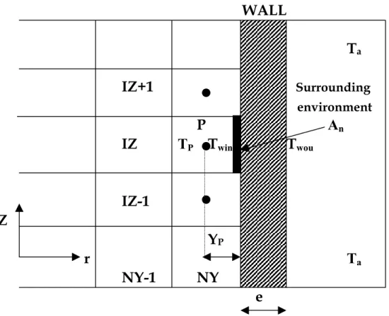
The conjugate heat transfer term is used to describe the process involved in the temperature variations in the solid and in the fluid. For describing it inside the conduit, a source term is introduced in the energy equation for the last point in the radial direction r. This term represents the conduction flux through the cylindrical wall in this direction (figure 2).

(

T T

)

IZ NY A e Y IZ NY S _{n Wou} S f S P  −       + = − * ) , ( * ) , ( 1

λ

λ

Sp is the source term for energy equation, e the thickness of the wall, Y the

distance of the last point close to the surface of the wall, the lateral surface of the last cell,

S

A_n

NYthe index of the near wall point in the direction corresponding to Y = R-r and IZ the index of the point in the Z direction, T the computational cell temperature and T_Wou is the outer wall temperature.

S f

λ

λ

, represent the thermal conductivity respectively in the fluid and the solid. The external temperature is fixed to the constant ambient value T_Amb(298°K) at the external boundary of the computational domain. The temperature at the outer wall

is computed by establishing the thermal balance through the use of an exchange coefficient h corresponding to the Biot law for the flux, which is fixed 5 W/m

Wou T

2

E

XPERIMENTAL STUDY

EXPERIMENTAL SET UP

This study was carried out in a full-scale experiment (Figure 1). A glass conduit is connected to a high efficiency gas boiler operating at low power (23 kW). The dimensions of the conduit are 9.20-m height, 0.13-m inner diameter, and 5-mm thickness of the wall. The comparison with numerical results is made in a domain of 8-m height.

The boiler works either in continuous established mode (steady state), or in cyclic running mode (unsteady state). The latter case was obtained using a programmed device for both running / non-running cycles. The device allowed imposing regular working periods.

Natural gas was chosen as a combustible for the first study. Compared to fuel, gas generates a less aggressive smoke on the sensors and has a simpler behaviour for the condensation process as a whole.

At the entrance of the conduit, the smoke had an average temperature in the centre of approximately 80°C and a velocity around 1m.s-1. Further details on the experimental set up may be found in (MAREF [2]) and(MAREF et al. [11]).

M

EASUREMENT

U

NCERTAINTIES

Different temperature fields (figure 3) were measured (smoke, interior and exterior wall, ambience), in 4 sections situated at 1 m, 2 m, 4 m et 8 m from the bottom of the conduit.

The measurements of temperatures were difficult to implement owing to the humid and corrosive environment, to which the different sensors were exposed. We used thermocouples type k imbedded in the wall or placed on prongs inside the conduit. An appropriate envelope face to the acid corrosion protected the sensors.

These probes were directly related to a computerised centre, which recorded regularly all thermocouples in use. After calibration of the whole system, it has been used for providing the temperature fields during the transient runs. However, calibration was not easy task in this environment and we have adopted uncertainty values that are usually met in the literature for such probes that are for temperatures. K 2 . 0 ±

RESULTS AND DISCUSSION

The profiles at the entrance section of the conduit (z=0), for the two continuous and cyclical regimes, were used as boundary and initial conditions for the numerical calculations. In the following, the numerical results of thermal fields were compared to the experimental data. But first, in order to provide a general overview of the phenomena, qualitative plots of the mean fields for the steady state calculation is presented (figure 4).

The temperature field exhibits a regular decrease on the axis and towards the wall of the conduit. One observes that the temperature fall along the conduit axis is around 18°K, a value that will be confirmed by the measurements. The effect of convection is rather obvious and the isotherms are nearly parabolic with maximum values on the axis. At the wall, a nearly isothermal value is found that differs from the ambience by about 15°K. The isotherms outside the conduit are almost parallel to the conduit direction at a short distance from it.

STEADY STATE

Figure 5 shows the experimental and numerical radial profiles of temperature for the three levels z = 0 m, z = 1 m, 3 m and 8 m. Good agreement is found between the experimental data and the calculation.

It has been shown previously by the authors (MAREF et al.[11]) that the actual flow in

the conduit induces condensation at the wall with a high saturation degree. Comparison with the dry air computed by the numerical model is surprisingly good. Although the model cannot describe the entire consistency of the actual physical phenomenon, this result shows that, as far as the thermal flow is concerned, it provides a sufficiently fair prediction to be used as a coarse approximation for design purposes.

UNSTEADY STATE

The explored regime corresponds to a cyclical running mode of the boiler characterised by a period of 15-min (5 min running and 10 min not running). The observation period covers eight cycles for simulating an actual run of two hours of the boiler.

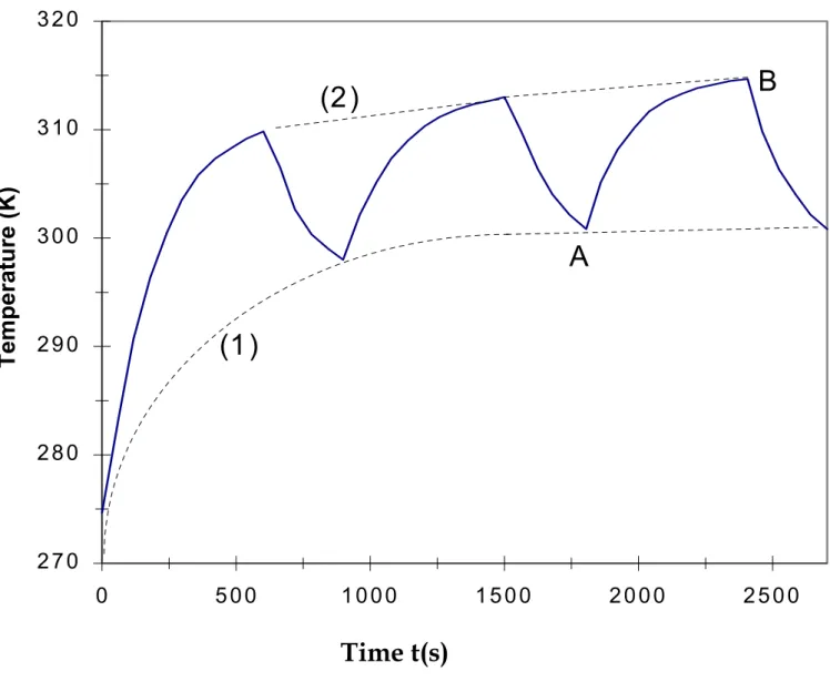
The typical transient behaviour of the thermal field is represented in figure 6 at the exit section and at the centre of the conduit. The duration of observation goes from rest to the periodic regime. Dashed curves (1) and (2) represent the upper and lower limits of the temperatures during the run. During the transient, a rise is observed in both limits of temperature. We can also observe a gradual increase of temperature during the heating phase and a quite abrupt fall when the boiler is stopped.

The comparison between numerical and experimental results is provided in figures 7 and 8. It is possible to distinguish between the previous transient stage, which lies approximately over three running periods and the established regime corresponding to the last fiveperiods. This comparison shows that some differences exist between experiments and computations during the first phase of heating from rest. These differences are limited to approximately 2.3 %. When thermal equilibrium is reached, they are reduced to 0.8 %. As a matter of fact, one can conclude that the agreement between experiments and computations is good.

Note that the time for thermal equilibrium is not identical for the whole levels of the conduit (figure 7). For example, the equilibrium is reached after 60 min at the bottom of the conduit (z = 1 m) and after 90 min at the upper part of the conduit (z = 8 m). There are also some differences between the evolution on the axis and near the wall as can be seen on figure 8. In general the simulations under-estimate the temperatures in the transient phase but are relevant to the final steady regime.

Nevertheless, these results also confirm that the approximation of dry incompressible gas used in this study conveniently predicts the thermal field.

C

ONCLUSION

The objective of this work is to develop and validate a simplified model for describing and predicting the thermal heat transfer in a smoke conduit. The work includes both established steady regime of operation, which serves as a reference basis, and the cyclic regime. The later is closer to the actual runs of the burner in its daily operation. The good agreement between computed and measured temperature leads to the conclusion that this numerical model is able to predict qualitatively the thermal distribution in the conduit. This information is useful in order to predict the places where condensation arises corresponding to low temperature zones (MAREF & al. [11]). Moreover it is suitable for intermittent regime in the normal use of the plant. That means that the switching time of the boiler is very large with respect to the turbulence time scales inside the conduct. Some results not presented here (CHERKAOUI [12]) (CHERKAOUI & al [13]) have shown that this model can also be

adapted to other situations with different materials for the conduct or other combustion products. One may think that some more elaborate model would give more accurate insight into the physical problem taking into account that two phases flow and low Reynolds number approach near the wall. Nevertheless, even though the present approach does not describe accurately the entire physical process, it provides a good design tool for the problem of exhaust of combustion products in domestic heating boilers.

ACKNOWLEDGEMENT

The authors thank the CSTB(Centre Scientifique et Technique du Batiment) in Marne La Vallée (France), the Direction of research of Gaz de France and Ugine (division d’Usinor Sacilor) for their technical and financial support. They are also greatly indebted to Mr Jacques Chandelier who initiated and directed this work.

REFERENCES

1. Cherkaoui H. (1), Maref W., Boisson H.C., Crausse P., Benjelloun Y. (1997) “Condensation de l’acide sulfurique dans un conduit d’évacuation des gaz de combustion.” Rev Gén Therm, vol 36, n° 10, November, 771-781.

2. MarefW. (1996), Modélisation des champs thermique et dynamique des Écoulements turbulents en régime instationnaire dans un conduit de fumée : Contribution à l’étude du phénomène de condensation des gaz de combustion. thèse de doctorat, INP – Toulouse, N° d’ordre 1162.

3. Phoenics, A Parabolic, Hyperbolic Or Elliptic, Numerical and Integration code series User’s manual TR/300

4. Launder B.E. et Spalding D.B. (1972), Mathematical models of turbulence. Academic Press, London.

5. Patankar S.V. (1980) Numerical Heat Transfer and Fluid Flow Hemisphere Publishing Company", Washington, USA.

6. Morgan V.T. (1975) "The overal convective heat transfer from smooth circular cylinders", Adv. Heat Transfer, Vol. 11, pp. 199-264.

7. Dyban E.P. et Epik E. Ya. (1970) "Some heat transfer features in the air flows of intensified turbulence", Proc. 4 th Heat Transfer Conference. F.C.5.7, Part 2, Paris-Versailles

8. Hinze J.O (1987) "Turbulence", McGraw-Hill, New York (1951), reissued.

9. Comings E.W., Clapp J.T. & Taylor J.F. (1948) "Air turbulence and transfer processes flow normal to cylinders", Indust. Engng Chem., Vol. 40, pp. 1076-1082.

10. Reynolds A.J. (1974) "Turbulent flows in engineering", A Wiley-Interscience Publication.

11. Maref W., Boisson H.C., Crausse P. et Chandellier J., (1995) “Experimental study of condensation phenomenon in chimney conduit”, Eurotherm N°47, "Heat Transfer in Condensation”, Paris, 4-5 October 1995.

12. Cherkaoui H. (2), Maref W., Chandellier J. (1997)“Contribution à l’étude du phénomène de corrosion dans les conduits de fumées: caractérisation théorique et expérimentale de la condensation des acides sur les parois.” Rev. Etudes et Recherches-Cahiers du CSTB N° 2984, October, PP 1-39

13. Cherkaoui H. (3), Maref W., Chandellier J. (1998)“Corrosion des conduits de fumée métalliques: essai simplifié.” Rev. Etudes et Recherches-Cahiers du CSTB N° 3066, September, PP 1-47

TABLE OF FIGURES

Figure 1 Scheme of domestic heat installation Figure 2 Conjugate heat transfers at the wall Figure 3 Thermocouples positions

Figure 4 Thermal field isotherms (unit in K)

Figure 5 Experimental and numerical results for temperatures at z = 1m, z = 3m, and

z = 8m

Figure 6 Computed rise of temperature at the centre of conduct (r = 0 and z = 8m)

Figure 7 Experimental and numerical time evolution of temperature at the centre of

the conduct at three vertical location (z = 1m, z = 3m and z = 8m; r = 0mm)

Figure 8 Experimental and numerical time evolution of temperature for z = 3m

Conduit wall 0.13m e D = 0.20 m Ambient air 8 m Analysed domain

WALL

T

a

IZ+1

Surrounding environment

P

A

n

IZ

T

P

T

win

T

wou

IZ-1

Z

Y

P

r

T

_a

NY-1

NY

e

0.2 m

Z

=

8

m

Section

4

Roof

5 m

2

nd

_floor

Thermocouples

Z

=

3

m

Section

3

2 m

Z

=

1

m

Section

2

1 m

Z

=

0

m

Section

1

1 m

G

roundfloor

Flow smoke

Figure 3 Thermocouples positions

315 320 325 330 335 340 345 0.00 0.01 0.02 0.03 0.04 0.05 0.06 0.07

Distance from the centre (m)

Temperature (K)

Z = 8 m Z = 3 m Z = 1 m Z = 0 m

Figure 5 Experimental and numerical results for temperatures at z = 1m, z = 3m, and

2 7 0

2 8 0

2 9 0

3 0 0

3 1 0

3 2 0

0

5 0 0

1 0 0 0

1 5 0 0

2 0 0 0

2 5 0 0

T e m p s t(s)

Température (K)

(1 )

A

B

(2 )

Time t(s)

270 280 290 300 310 320 330 340 0 1000 2000 3000 4000 5000 6000 7000 Température (K) z = 1 m z = 3m z = 8 m

Time t(s)

Figure 7 Experimental and numerical time evolution of temperature at the centre of

♦

T

win

Exp

Tf[r=0] Exp

T

win

Sim

Tf[r=0] Sim

Tp T

Time t(s)

₄ 280 285 290 295 300 305 310 315 320 325 330 0 1000 2000 3000 000 5000 6000 7000 Température (K) Tf[r=0] sim int pint exp Tf[r=0] exp r = 0 mm r = 65 mm

p

Figure 8 Experimental and numerical time evolution of temperature for z = 3m