Constraint satisfaction modules : a methodology for analog circuit design

Constraint Satisfaction Modules:

A Methodology for Analog Circuit Design

by

Piotr Mitros

B.S., Electrical Science and Engineering (2004)

M.Eng., Electrical Engineering and Computer Science (2004) Massachusetts Institute of Technology

Submitted to the Department of Electrical Engineering and Computer Science in partial fulfillment of the requirements for the degree of

Doctor of Philosophy in Electrical Engineering and Computer Science at the

MASSACHUSETTS INSTITUTE OF TECHNOLOGY September 2007

@ Piotr Mitros. 2007. This work is licensed under the Creative Commons Attribution 3.0 License. A copy of this license is provided in Appendix D. The author hereby grants to MIT permission to modify, sublicense, reproduce, and distribute publicly copies of this thesis document in whole or in part in any medium

now known or hereafter created.

Author ...

...

..

...

... ...

Department of Electrical Engineering and Computer Science

--

-August

30, 2007

Certified by..

.. ..

... .

.

.

.

.-..-...

Gerald Jay Sussman

Panasonic Profe sor of Electrical Engineering

-

Thesis Supervisor

Certified by .

homas F. Knight, Jr

r-en' earst

Accepted by... ...

...

-.

HUSErTS

,rruT1,,•

Arthur C. Smith

or~HwN v

Chairman, Department Committee on Graduate Students

CTR 1;2 2007

Constraint Satisfaction Modules:

A Methodology for Analog Circuit Design

by

Piotr Mitros

Submitted to the Department of Electrical Engineering and Computer Science on August 30, 2007, in partial fulfillment of the

requirements for the degree of

Doctor of Philosophy in Electrical Engineering and Computer Science

Abstract

This dissertation describes a methodology for solving convex constraint problems using analog circuits. It demonstrates how this methodology can be used to design circuits that solve function-fitting problems through iterated gradient descent. In particular, it shows how to build a small circuit that can model a nonlinearity by observation, and predistort to compensate for this nonlinearity. The system fits into

a broader effort to investigate non-traditional approaches to circuit design. First, it breaks the traditional input-output abstraction barrier; all ports are bidirectional. Second, it uses a different methodology for proving system stability with local rather than global properties. Such stability arguments can be scaled to much more complex systems than traditional stability criteria.

Thesis Supervisor: Gerald Jay Sussman

Title: Panasonic Professor of Electrical Engineering Thesis Supervisor: Thomas F. Knight, Jr

Acknowledgments

I would first like to thank Professor Gerald Jay Sussman. Gerry has been my mentor since I arrived at MIT as a freshman. He has always gone to great lengths to help me with problems, both research and personal. Without his help and guidance, this thesis would have been impossible. Gerry is a brilliant scientist, an amazing teacher, a great supervisor, and most importantly, a good friend.

Next, I would like to thank Tom Knight. I have known Tom for almost as long as Gerry. In that time, Tom has gone significantly out of his way for me a number of times. When I ran out of funding one semester, he was able to miraculously find new funding on short notice. At one point, he taught a class on digital circuit design simply because a couple of friends and I asked him to. He even rescheduled it to before he would normally wake up so that I could attend. Tom is an amazing person. I'd like to thank Steve Leeb for agreeing to be on my thesis committee, for su-pervising my RQE exam, and otherwise being a great guy. In addition, I'd like to thank the many people with whom I've discussed this thesis, and who helped guide its direction. I'd like to single out Al-Thaddeus Avestruz, John Wyatt, Neil Ger-shenfeld, and Xu "Andy" Sun. In addition, I'd like to thank those professors who took the time to guide me before I began work on this thesis. In particular, I'd like to thank Hal Abelson for his guidance over the years, as well as his help in finding funding for the last two years of my undergraduate studies. I would like to thank Rafael Reif. Rafael supervised my research for a year. In that time, he was always kind and fair to his students, and his guidance was invaluable in choosing my research goals and professional career path. I also wanted to thank Anant Agarwal for his help with admissions to the Ph.D. program. Finally, I'd like to thank those who set me on this path, and in particular Walter Bender of the Media Lab (now One Laptop per Child), John Gibson of Landmark Graphics Corporation (later, Halliburton, and Paradigm), as well as the staff of the Research Science Institute, for their guidance and support while I was still in high school. Last, I would like to thank Jesus del Alamo for providing funding through the iLabs project while I did this research, and

for giving me the opportunity to see the world.

Finally, I'd like to thank my family. First of all, I'd like to thank Stefanie Tellex for her love and support over the past three years, as well as always being willing to help code before a deadline. I'd like the thank my sister Ania for always being there to listen to my personal problems, as well as for the many technical discussions about both of our dissertations. I'd like to thank my father, Jozef Mitros, who was always ready to assist me throughout the program with advice about my life, as well as with explanations of device physics and fabrication. Finally, I'd like to thank my moom, Katarzyna Mitros, for her moral support and her faith in me throughout the process.

Contents

1 Introduction 15

1.1 System Overview ... 16

1.1.1 Constraint Optimization Solver . ... 16

1.1.2 M odeling . . . 18

1.1.3 Linearization .. ... ... ... .. ... .. ... ... . 18

1.2 M otivation . . . . . . .. . . 20

1.2.1 Analog Architectures ... .... 20

1.2.2 Breaking the Input-Output Abstraction . ... 22

1.3 Background ... ... 23

1.3.1 Neural VLSI Systems ... 25

1.3.2 Passivity and Other Stability Methodologies . ... 27

1.4 Lim itations . . . .. . 31

1.5 Document Overview ... 33

2 Static Case - Constrained Problems 35 2.1 Design Discipline ... 36

2.2 Stability Analysis ... 37

2.2.1 Robust Low Frequency Stability . ... 38

2.2.2 Saturation Behavior ... 42

2.2.3 High Frequency Stability ... 43

2.3 Test Circuit . . ... .. . . . .. . . .. .. . . . .. . . . .. . .. . 44

2.3.1 Circuit performance ... 46

3 Dynamic Case - Function Fitting

3.1 Stability for General Linear Regression 3.1.1 Definitions and Notation . . . . 3.1.2 Robust Continuous Time Stability 3.1.3 Robust Discrete Time Stability . . 3.2 Parallel Equivalent Model . . . . 4 Linearization

4.1 Circuit Compilation Overview . . . . 4.2 Optimality . ...

4.3 Robustness ...

4.4 Circuit Implementation ... 4.4.1 Properties of the Circuit ... 4.4.2 Experimental Results ...

5 Conclusion

5.1 Improved Operational Amplifier . . . . 5.1.1 Improved Matching ...

5.2 Controlling Systems With a Time Delay 5.2.1 Cartesian Feedback ...

5.3 Other Applications ... 5.4 Future Theoretical Work ...

5.4.1 Integration with Digital Techniques 5.4.2 Improved Performance ...

5.4.3 Further Simplifications ...

5.4.4 Generalizing to Dynamic Systems . 5.4.5 Dynamic Constraints . . . . 5.5 Summary ... A Cast of Characters B LaSalle's Theorem 49 . . . 52 . . . 52 . . . 53 . . . 55 57 61 . . . . . 63 . . . . 65 . . . . 67 . . . . 68 . . . . 72 . . . . 73 75 . . . . . 76 . . . . 80 . . . . . 82 . . . . 82 . . . . 84 . . . . 84 . . . . . 85 . . . . 86 . . . . 90 . . . . . 92 . . . . . 96 96 99 101

C Sample Circuit Implementations 103 C.1 Squarer ... ... 103 C.2 Exponentiator ... ... ... 104 C.3 Multiplier ... ... ... 104 C.4 Soft Equals ... ... 105 C.5 Approximately Equals ... ... 106 C.6 Less-Than or Equals ... ... 106

List of Figures

1-1 Block-diagram of a 2-port element . ... . 16

1-2 System for solving a network of equations . ... 17

1-3 Function fitting circuit ... ... ... .. 18

1-4 Combination function fitting and linearization circuit . ... 19

1-5 Double-width operational amplifier. ... ... 21

1-6 ax + by = z expressed with transformers ... . . . . 23

1-7 Counterexample circuit to control passivity . ... 29

1-8 Objective function with two minima . ... 31

1-9 IV characteristics of an active 1-port . ... 32

1-10 Counterexample circuit to circuit passivity . ... 32

2-1 Region B' in robust stability ... 40

2-2 Level curves in robust stability argument. . ... 40

2-3 Region B' and B1 in the robust stability argument . . . . 41

2-4 Active Transformer ... 42

2-5 Circuit holding the constraint 2x = y . ... 44

2-6 Circuit holding the constraint x - y = z . ... 45

2-7 Circuit holding the constraint x + y + z = 4 . ... 45

2-8 Photo of static constraint circuit ... .. 46

2-9 Scope traces of static constraint solver . ... 47

3-1 Graph showing iterated gradient descent . ... 50

3-2 Illustration of a ball around a function . ... 53

3-4 Projection of an estimate onto the hyperplane generated by a point in the ball around a function . . ...

3-5 Projecting onto 4 lines around a ball of radius r . ... 3-6 Basic modeling system ...

3-7 Equivalent modeling system, with switched constraint blocks . . . . . 3-8 Equivalent modeling system, limit case of fast switching . . . . 3-9 Illustration showing that order of inputs effects convergence time . . . 4-1 Compensating for a nonlinearity. . . . . 4-2 Block diagram of function-fitting and linearization circuit . . . . . .

4-3 Circuit demonstrating robustness-by-voting . . . . 4-4 4-5 4-6 4-7 4-8 5-1 5-2 5-3 5-4 5-5 5-6 5-7 5-8 5-9 5-10 5-11 5-12 5-13 5-14

Block diagram of simplified linearizer . . . . Circuit detail of simplified linearizer . . . . Photo of simplified linearizer . . . . Input-output relationship of linearized nonlinearity Scope traces of dynamics of linearizer . . . . Conventional operational amplifier . . . .

Operational amplifier with monitored distortion . . Multiple differential pairs in parallel . . . . Different differential pairs in parallel . . . . A complex super-linearized stage . . . . Multiple differential pairs in parallel with switches . A system with a time delay ...

Block diagram of Cartesian feedback . . . . Example of spatial parallelism . . . .

58 58 58 60 62 65 68 70 70 71 73 74 . .. 77 78 . . . 79 . . . 79 . . . 80 . . . 81 .. . 82 . . . 83 . . . 87 Spatial parallelism improving convergence speed in a single circuit. . . Soft-equals in parallel circuit ...

Simplified learning system assuming fi(yd,,e) = fi(y) .. . . . . Simplified learning using switches . . . . Simple linearization block equivalent to LTI system . . . .

87 89 91 91 93 ' ' ' ' ' '

5-15 Dominant pole LTI controller ... 93

5-16 Controller for nonlinear systems with memory . ... 94

C-1 Squarer circuit ... ... ... 104

C-2 Soft equality ... ... 105

C-3 Softer soft equality ... ... 106

C-4 Diode as less-than-or-equal constraint . ... 107

Chapter 1

Introduction

This dissertation presents a methodology for the design of analog circuits. Under this methodology, the ports of all circuit blocks are bidirectional. The stability of circuits designed following this methodology can be determined by local, rather than global, analysis. If the circuit blocks follow a certain design discipline, they can be connected in nearly arbitrary configurations while maintaining stability. This methodology may be applied to designing circuits that solve several classes of problems. In particular, it is applied to designing a small circuit that can build a model of a memoryless nonlinear system, and to predistort to linearize this system.

First, this document shows how this methodology can be used to solve basic con-strained optimization problems in analog circuits. Given a set of constraint equations, it shows how to build a circuit that will solve that set of equations. This circuit is sufficiently small that it can be used for simple analog processing in basic analog circuits; for instance, it may be used to set optimal bias currents for another circuit. Next, this thesis shows how to use this methodology to build a circuit that can be used to determine the parameters of a model of a system through observation of the system's behavior. This circuit can, for instance, be used to monitor and model the nonlinearity of the power output stage of an amplifier. Given this model, a symmetric, matched circuit can predistort to compensate for the nonlinearity.

These circuits are small enough that they can be used as blocks for other analog circuits, particularly in places where digital processing is impossible due to size and

1(V1, V2) Control 2(VM, V2)

1-- f-2

Figure 1-1: A block-diagram of a 2-port element. A controller monitors the voltage at the adjacent nodes, and injects current into both nodes if a constraint is not met. cost constraints. They also lend themselves well to automated synthesis.

1.1

System Overview

This section begins with an overview of the constraint equation solver, and later develops it into the modeling and linearization circuits.

1.1.1

Constraint Optimization Solver

The constraint optimization circuit solves systems of simultaneous equations and inequalities. Given n constraints, the circuit is composed of n blocks, each corre-sponding to a constraint. Each of these blocks has mi ports, where mi is the number of variables in the ith equation. Each block then attempts to hold the constraint cor-responding to this equation by measuring the voltage on each port, and generating an error current feeding back into that port. This error current moves the voltages in the correct direction to meet the constraints. This can be viewed as a generalization of the concept of a transformer. The block-diagram of a 2-port block is shown in Figure 1-1.

Each block is assigned an objective function Li(Vp1, VP2, ..., VPN) that describes

how well the constraints in each block are met (e.g., the square distance from the constraint). Li achieves its minimum when the constraints are completely met. The current output from each block through each port is then proportional to - _dVpidL1

where Vpi is the voltage seen at that port1. Inequalities are approximated by crafting

'This may also be implemented with the dual circuit, swapping currents with voltages, and capacitors with inductors.

I1~

Figure 1-2: A system for solving a network of equations consisting of connected constraint blocks.

appropriate objective functions.

Take the constraint Vp₁ = 2. VP2 (in other words, a block behaving as a 2:1

trans-former). One possible objective function is Li(Vp1, VP2) = (Vp - 2 -Vp2)2. Then,

to implement this constraint, the block shown in Figure 1-1 should be implemented with a controller that will output the current equal to Ip1 = -ydL = -2Vp1 + 4VP2

and IP2 = -- 8VP2 + 4VP1. Notice that, as with a physical 2:1 transformer, the

currents have a 1:2 ratio.

These blocks can tie together into arbitrary networks to solve more complex con-straint problems. For instance, the network shown in Figure 1-2 will solve the set of equations:

x2 =y, x+y=z, z-=a+b

c = 1, x = ab, b4 _{+ b}2 _{= C}

If the objective function associated with this set of equations were convex and had a unique solution, this network would find that solution. In this case, assuming least squares objective functions, the objective function is not convex. It has a discrete set of local minima, and therefore the network will converge to one of these local minima. If the system were underconstrained such that the objective function had a connected subspace where it was minimized, the system would enter a minimum, but could drift through the subspace associated with that minimum.

If the system of constraints is strictly convex, systems of this form are stable. This criterion is sufficient, but not necessary - a number of non-convex constrained and

t Parameters

It

Parameters

Figure 1-3: This is a function fitting circuit. It consists of an underconstrained constraint block monitoring a system. In this case, the system will find the parameters

b and c of the affine model y = bx + c of the system by iterated gradient descent.

overconstrained systems can be solved as well.

1.1.2

Modeling

This section describes how to build circuits that can model systems by observation. The circuits described can be connected to multiple terminals, monitor those termi-nals, and develop an approximate model of the relationship between the voltages on those terminals. The circuit is primarily useful for memoryless models, but can model a variety of functions, including a superset of general linear regression.

The model parameters are found using the same type of circuit as described in Section 1.1.1, but operating over a set of underconstrained equations. An example of this procedure is shown in Figure 1-3.

Here, as x and y change, the system continuously moves b and c towards the line defined by y = bx + c. This procedure is a form of iterated gradient descent. For a large class of models (a superset of general linear regression) it will find what is, in at least one sense, an optimal estimate of the parameters of the model of the original system.

1.1.3

Linearization

Once one can function-fit a nonlinearity, it is often straightforward to invert it, as shown in Figure 1-4. Here, the top block builds a model of the nonlinearity, while the bottom block inverts the function. Since the blocks are bidirectional, the top block

Ydesired

Figure 1-4: Shown is a circuit that can build a model of a nonlinearity, and predistort to linearize it. Since the modeling circuit is bidirectional, an identical, matched circuit is used to implement the model, predistorting to linearize the nonlinearity.

and bottom block may be implemented as identical, matched circuits. The buffers in Figure 1-4 are not necessary. They are included in the figure primarily to show direction of flow of information, and to simplify explanation and analysis.

One caveat is that not all models can be inverted. While monotonic models are invertible, non-monotonic models may have multiple local minima. In that case, the matched block may become trapped in one of those minima.

It is possible to compile most circuits designed under this methodology into a more efficient implementation. Many blocks contain redundant components already contained in adjoining blocks, which may, instead, be shared. In addition, for many constraints circuits, approximations can significantly reduce circuit complexity. Chap-ter 4 will work through an example of this procedure by taking a simple second order Taylor series linearizer circuit, and compiling it down to an implementation that requires about a dozen major components (operational amplifiers or Gilbert multipli-ers). This implementation will also further improve matching, since many calculation will be shared among blocks.

As shown, this technique is useful for controlling nonlinear memoryless systems. There are natural ways of extending the work to systems with memory, but these are not yet fully .developed, and so will not be explored in this thesis.

1.2

Motivation

One goal of this work is the exploration of analog techniques that scale to more com-plex systems. The use of a local stability criterion may allow the construction of much more complex analog circuits than would be possible with traditional loop-shaping techniques. In addition, the work explores several other areas of unconventional cir-cuit design, such as breaking the input-output abstraction barrier.

1.2.1

Analog Architectures

Moore's Law scaling has been much more generous to digital systems than to analog systems[l]. Moore's Law benefits circuit designers in two ways:

* More transistors * Better transistors

While analog circuit design has been able to take advantage of better transistors, it has not been able to exploit the advantages brought by the increased number of transistors as well as digital electronics has2. There are a number of reasons for this problem, but probably the most important one is that existing analog circuit design methodologies are optimized for extracting optimal performance from circuits consisting of a small number of devices. As a result, they do not scale to very large circuits. The problem of determining stability grows very quickly with the complexity of the circuit. Simulators do not perform well on complex circuits3_{. As a result,}

almost all progress in circuits is either from device improvements, or small topology optimizations. Compared to digital, little progress (beyond integration) comes from advances at an architectural level.

The utilization of more devices is grossly inefficient. For instance, to achieve better matching of devices in an operational amplifier, the standard approach simply dou-bles the size of all devices, effectively building two operational amplifiers, connected

2

There are some exceptions to this generalization. For instance, flash ADCs use large amounts of parallelism to achieve high conversion rates.

3

Their poor performance is most likely due, in part, to their inability to extract simple models of subcircuits.

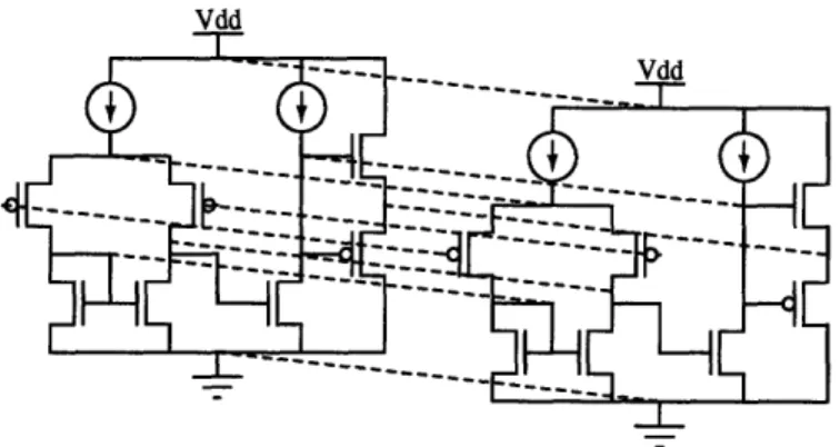
Figure 1-5: In traditional circuit design, to improve matching between components, devices are simply increased in size, or multiple devices are placed in parallel, as shown in this double-width operational amplifier.

together at all matching nodes, as shown in Figure 1.2.1. This design technique is almost certainly not the most efficient way to design a circuit. One could, instead, try connecting two different operational amplifier designs, one with high bandwidth, and the other with low distortion, in some clever way to build a single operational amplifier with high bandwidth, but low distortion at low frequencies.

Many techniques for exploiting complexity exist. Multiple amplifiers on a trans-mission line, to form a distributed circuit, as shown by Percival[27] and popularized by Hajimiri[15], can substantially improve bandwidth over traditional techniques. Distributed circuits can route signals outside the normal signal path to introduce an effective negative time delay. Kim[23] built a high-performance ring oscillator based on this technique. Systems may also include large amounts of additional analog com-putation around a conventional circuit in order to fine-tune bias levels, cancel out distortion, and do other types of processing to aid in circuit operation. Similar tricks are commonly used in digital circuits, where advanced branch prediction algorithms and LRU cache schemes are placed outside of the main signal path to maximize the performance of a simple microprocessor core. Similarly, a processor may have multi-ple execution units, or more recently, multimulti-ple cores, and route tasks to whichever is idle. This sort of efficient use of parallelism is rare in analog design.

Hundreds of similar techniques that tradeoff circuit complexity for better perfor-mance exist. Each is very effective in isolation. Few circuits, however, exist that

exploit a significant number of these techniques - designing such a circuit, and fur-thermore, determining its performance and demonstrating its stability is simply too hard.

The field of electronic engineering requires a new set of methodologies, abstrac-tions and mathematics that will allow the design and synthesis of complex, intercon-nected, stable systems, and the characterization of their performance. In this paper, I present one such methodology. I believe that other methodologies may also be created, especially deriving from work in distributed dynamics of complex systems, and in particular, from the areas of SIMD systems, amorphous computing, and dy-namics of two-dimensional physical systems. These methodologies, or others like it, may eventually allow the construction, or perhaps more importantly, the automatic synthesis of complex circuits that will achieve drastically higher performance than

traditional analog design techniques.

1.2.2

Breaking the Input-Output Abstraction

Traditional circuits are built based on an input-output abstraction. Analog circuit design relies on guard-rings and other complex structures to minimize coupling be-tween parts of the circuit. Feed-through from the output of an amplifier to its input is generally viewed as an undesired interfering signal.

Especially in high-end RF systems (in particular in MIMO), feed-through very significantly limits performance. Conventional approaches try to solve this by min-imizing the level and effect of feed-through. An alternative way to deal with this problem is to try to control and understand the effects of feed-through, and poten-tially try to exploit them.

S-parameter models do this to a limited extent, but are primarily used in LTI systems, such as gain blocks or filters, rather than for nonlinear blocks that perform actual computation, such as modulation or demodulation. Treating all ports as both inputs and outputs may eventually give rise to a powerful new set of circuit design techniques where feed-through is a desirable, controlled design parameter, rather than

+

Figure 1-6: The constraint ax + by = z expressed with transformers.

1.3

Background

This work is based on the traditional technique of solving systems of linear equations using transformers. This method was introduced by Mallock[24], and was common use in the early days of analog computing, but died off as the input-output abstraction took over in the forties and fifties. Seidel and Knight revived it by reimplementing this type of circuit in an IC using switched capacitor transformers[29]. They expressed constraints such as ax + by = z using a pair of transformers, as shown in Figure 1-6.

Their circuit consisted of multiple transformer blocks like this and solved arbitrary linear equations. This approach allowed for some basic nonlinearities - for instance, diodes could be used to express inequalities - but as presented, it did not directly scale to arbitrary nonlinear constraints.

My approach is a direct extension of Seidel and Knight's work. My first step was to replace the switched capacitor transformers with active transformers. This was not entirely novel - for instance, Chua, et al.[7] build a transformer with many ports, and showed that it could be used for mathematical programming. Developing active transformers lead to a number of issues. First, while physical transformers are passive, an active circuit approximating a transformer may no longer be passive if the implementation is off by an arbitrarily small e. Therefore, stability can no longer follow from passivity. Second, the definition of a transformer in terms of voltage and current ratios is slightly ambiguous. If a 2:1 transformer is driven with 1V on one side, and 1.5V on the other side, it needs to output reasonable currents. Whether those currents should be in a ratio of 1.5:1, or 2:1, or otherwise, falls outside of the traditional definition of a transformer. These issues lead to the general formulation of transformers found in this thesis. This formulation includes the non-linear (and not

necessarily energy-conserving) generalizations thereof. Finally, once this definition was in place, I noticed that this approach generalized to the problem of modeling, and therefore, linearization.

There is a wide body of prior work that attempts to solve problems similar to the one presented in this thesis. Researchers from a variety of fields have, independently, worked on circuits similar to those in this thesis, circuits that solve similar problems in other ways, or worked on mathematics relevant to these circuits in domains outside of electronics.

Dennis's seminal Ph.d. thesis[11] was one one of the first papers on solving math-ematical programs with electrical networks. In his thesis, Dennis proves that any direct current network made up of voltage and current sources, ideal DC transform-ers, and ideal diodes is equivalent to a pair of dual linear programs. A network made up of linear resistors together with these elements is equivalent to a pair of dual quadratic programs. Conversely, he shows that any linear or quadratic program may be modeled by an electrical circuit. His thesis begins to approach the problem of more general nonlinear mathematical programming, taking two significant steps. First, he integrates a class of nonlinear resistors into his framework. Second, he shows how his work with linear components can be used to compute the direction of steepest descent. His circuits are much more compact than those in this thesis. He does not, however, approach the level of generality of this work.

The most important (although, unfortunately, not best known) work on solv-ing general nonlinear mathematical programs in analog circuits is Chua's canonical nonlinear programming circuit[6]. Chua developed a system for solving nonlinear programs that is very similar to the static case of the constraint solver in this thesis

- the mathematical model of an individual constraint block is essentially the same as in my circuit, although the mathematical foundations are slightly different, as are the circuit implementations. Chua's original paper was limited in the way that it treated stability - Chua shows that the system with no dynamics and no node capacitances would have an equilibrium operating point at the solution of the mathematical pro-gram, but other than citing general stability criteria from a previous paper[5], did not

give a way to guarantee that the equilibrium will be stable. Stability analysis, rather, had to be done on a circuit-by-circuit basis. In a later paper[20], Kennedy and Chua added node capacitance, and so were able to demonstrate stability in the general case in a manner very similar to that in this document. Further analysis of stability in the linear case may be found in Song[30], who performs a stability analysis from a control system perspective.

There are two minor extensions to Chua's work. Chua[3] published a paper show-ing how constraints and inequalities may be implemented within his framework. In this paper, he expresses constraints like f(x) > 0 as y = If(x)I or y = f(x)2_{, and}

min-imizes y according to his framework. Jayadeva, et al.[16] point out several problems with this approach. These problems mostly center around convex problems becom-ing non-convex and havbecom-ing multiple local minima, choice of how much weight should be given to the constraints, and computational complexity. To a large extent, these problems are more relevant in computer science contexts, where optimizers solve com-plex, poorly understood numerical optimization problems, than they are to circuits, where the problems are likely to be simpler, and better understood. The authors propose a solution, but it is not obvious how easy it would be to apply in a circuits context. Forti, et al.[14] extend Chua's work, somewhat theoretically, to non-smooth mathematical programming problems.

I found this work in fairly late stages of my thesis, and was pleasantly surprised to find that high quality work had been pursued in the area before. My thesis extends on Chua's in several ways. It is somewhat more general, especially in that it targets dynamic systems. The stability proofs in Chua's work (even in the latter papers) are also somewhat less developed.

1.3.1

Neural VLSI Systems

A large number of similar systems exist in the field of neural VLSI systems. There are dozens or hundreds of papers in this area, mostly of very low quality, so it is difficult to give a concise summary. The most important (and rather good) paper in this area is by Tank and Hopfield[17]. This paper presents a way of solving linear programming

problems using a circuit that consists of neural summing nodes, and inspired the vast majority of papers on solving constraints problems with neural VLSI. Chua published a careful analysis of Hopfield's circuit[19] that shows that it is nearly identical to a special case of the general solver shown in Chua's canonical nonlinear programming circuit[6], as well as, by extension, this thesis. The circuits differ in two significant ways. First, Tank's circuit is modularized by neurons, rather than by constraint blocks. This modularity makes it difficult to implement general nonlinear constraints, and Tank's circuit is therefore limited to linear (and very limited nonlinear) programs. Second, Tank's way of proving stability requires all variable nodes to have resistors to ground. This causes the circuit to generate approximate, rather than exact, solutions. Due to the difficulty of computing derivatives, a number of followup VLSI circuits rely on injecting noise to compute derivatives. For instance, Jelonek[18] created a system that uses an analog technique based on simulated annealing. First, large amounts of noise are added to come close to the global minimum. Smaller amounts of noise are then added to perform basic gradient descent to find a local minimum. In addition, a neural network holds constraints. The resulting circuit is moderately complex, and as a result, only simulation results are available.

Learning by gradient descent is a standard technique in the field of neural net-works. Two main techniques are back propagation and weight propagation. A good overview of neural network techniques may be found in any introductory artificial intelligence text, such as Winston[32] or Russell, Norvig[28]. These texts tend to be clear and concise, and put neural networks within the broader context of machine learning. Most neural network texts, in contrast, while more detailed, tend to under-state the limitations of neural networks, and do not adequately contrast them with other, similar machine learning techniques. The best work describing what percep-tions, the building blocks of neural networks, can and cannot do is by Minsky and Papert[26].

VLSI systems have been built around virtually all computer science neural network techniques. Most of these systems may be used for building models, and several can solve constraint problems. There is also a fairly large field of neural network-based

controllers. Since there is such a wide variety of work, it is difficult to make general comparisons to my work. One major limitation of these systems, in general, is that performance is difficult to characterize. While neural networks often perform very well, their operation is poorly understood. As a result, it is difficult to predict in what contexts they will work well, and the overall function of the system can often only be characterized experimentally. The problem is that the model being fitted to is not well characterized, or, in some cases, even deliberately expressed. Even if the model space is understood, it is often difficult to predict whether a given system will reach the global minimum, or some local minimum. As a result, in many cases, it is difficult to build a neural-network based system with deterministic performance.

1.3.2

Passivity and Other Stability Methodologies

There are a number of other criteria for designing complex, interconnected, stable cir-cuits. Digital circuit design uses a methodology that relies on locally stable elements and, within a given clock cycle, a one-way flow of information. Analog circuits may be integrated the same way - stable local elements with a one-way flow of information

- but this is usually only used to achieve greater system integration.

Passivity is a common criterion for achieving system stability. The word "pas-sive" has several meanings, depending on the domain. Each meaning has a different, associated set of stability theorems. In control systems and circuit network theory, a passive device is one that consumes, rather than produces, energy. Examples in-clude devices like transistors, tunnel diodes, and glow tubes, but exin-clude voltage and current sources. In contrast, in circuit design, passive devices are ones that are inca-pable of power gain. In circuit design, transistors, glow tubes, and tunnel diodes are considered active, whereas voltage and current sources are considered passive.

Passivity is a very powerful tool for demonstrating stability. It is used in a number of domains, including filter design, and control system design. Nevertheless, it is often inadequate for simulated passive devices, such as the ones in this thesis. As shown in the active transformer example, when active devices simulate passive ones, small variations from the ideal may make a system unstable, even if all devices are ideally

passive. This is especially a problem at higher frequencies, where actual behavior necessarily diverges significantly from desired behavior.

Control Systems Passivity

For the purposes of this discussion, define a resistor as a nonlinear memoryless 1-port4. A resistor is considered passive iff vi > 0 for all points (v, i) on its characteristic. It is considered strictly passive iff vi > 0, except at the origin.

The voltage within a network of passive resistors cannot exceed the voltages pre-sented on the terminals. The current within any resistor may not exceed the total current input through all ports. This is a strong bounded input/bounded output (BIBO) stability criterion.

Informally, an arbitrary n-port, with memory, is considered passive if it can store or dissipate energy, but cannot create energy. The formal definition varies between texts, and is often incorrect in the way in which initial conditions are handled. The best definition available is found in Wyatt [33]. Wyatt also explains the problem with other definitions. An abbreviated version of this definition follows.

The available energy from an n-port in state x is defined as:

EA(x) = sup

(v(t), i(t))

Where the notation supxT>o indicates the supremum is taken over all t > 0 and all admissible pairs v(t), i(t) with the initial state x. An n-port is considered passive if Vx, EA(X) < 00.

A network consisting entirely of passive elements is itself passive, and therefore, only a finite amount of energy can be drawn from it.

A resistor is considered increasing iff (v' - v")/(i' - i") Ž OV(v', i'), (v", i"), and

strictly increasing iff (v' - v")/(i' - i") > OV(v', i')

$

of strictly increasing two-terminal resistors and independent sources has at most one

4_{This definition varies between texts - many circuit theory texts consider all memoryless n-ports}

to be resistors, while many traditional circuit design texts require resistors to be linear memoryless 1-ports.

R

2V V

Figure 1-7: This circuit is a counterexample that shows that stability could not be shown by controls passivity. The voltage source shown holds the constraint V = 2, minimizing the objective function (V - 2)2. It is not, however, passive, since it may output energy.

solution. Furthermore, the slope of the transfer function 'in of a network made of strictly increasing resistors cannot exceed unity. This property is also sometimes called (strict) monotonicity and (strict) incremental passivity.

A formal discussion of passivity and monotonicity, although limited to memoryless 1-port elements, may be found in Chua, et al[4]. This is an excellent reference on the topic. Desoer and Kuh[12] proves the stability of networks consisting of capacitors, inductors, and nonlinear passive resistors. Cruz and Valkenburg[9] touches on multi-port elements, but does not develop very much theory about them.

Passivity forms a powerful discipline for designing stable systems. Indeed, it is one of the standard methods used in control systems. Khalil[21] includes a very accessible text on passivity in control systems. Although the discussion is inspired by circuits, the text primarily focuses on the design of stable control systems for traditional controls applications, rather than for electronic circuit design. Vidyasgar[31] is a more rigorous control systems book that also discusses stability by passivity, although the discussion is shorter than that in Khalil.

Circuits designed under the methodology presented in this dissertation are not passive in the control systems sense. A circuit implementing the constraint such as

x = _{2, with a least squares objective function, is simply a Thevenin voltage source,}

as shown in Figure 1-7. This block is trivially not passive in the controls sense, since it outputs power.

Circuit Design Passivity

In circuits terminology (in contrast to control systems), passive devices are ones not capable of gain, whereas active devices are ones capable of gain. For two terminal devices, this definition is identical to the one of monotonicity given above. I have not been able to find a formal definition for multi-terminal devices, but a suggested definition is that the small signal model is thermodynamically passive. Active devices, in circuit design terminology, include many dissipative devices capable of gain that would be considered passive by control and network theorists, including two-terminals such as tunnel diodes, glow tubes, and multi-terminal devices, such as transistors, relays, and tubes.

In addition to being another methodology for determining stability, the work in this thesis is built on passivity (in the circuit sense) - the work on solving constraints with transformers[29] upon which my work is based showed stability by passivity.

Nevertheless, even lacking a good definition for multi-port devices, it is easy to show that the methodology allows for non-passive components by constructing an active one-port. Take a circuit implementing the constraint associated with the

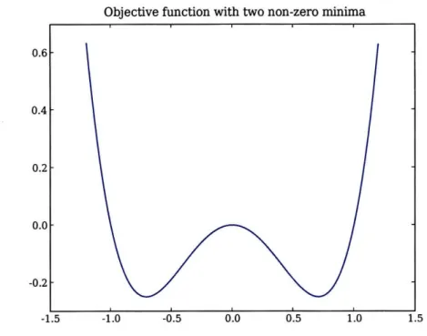
ob-jective function L(x) = - x2_{. This constraint, x , is shown graphically}

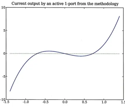
in figure 1-8. This objective function has two minima - ±. It has the voltage-current relationship I = 4V13 - 2_{Vx, shown in Figure 1-9. This is non-monotonic.}

Indeed, connected in parallel with an inductor and capacitor, it acts as an oscillator, as shown in Figure 1-10.

The methodology presented in this thesis is, also a generalization of the concept of a memoryless monotonic one-port. Given a memoryless monotonic one-port, with I-V characteristics i(v). Let:

L(xi, x2) = f (X 1 - 2 )i(x1 - v-

)dv

Then,

dL

= i(x₁ - x₂) dxl

Objective function with two non-zero minima 0.6 0.4 0.2 0.0 -0.2 -1.5 -1.0 -0.5 0.0 0.5 1.0 1.5

Figure 1-8: Shown is an example of an objective function with two non-zero minima.

A circuit implementing such an objective function will be non-passive in both senses.

And similarly,

dL

= -i(xl - x

)

Therefore, all incrementally passive one-ports are valid constraint block within this thesis methodology, and this thesis may be viewed as one generalization of the concept of incremental passivity".

1.4

Limitations

This approach is only proven to satisfy constraint optimization problems with uni-modal objective functions. Efficient general-purpose optimizers do not exist since the problem is NP-hard; it is trivial to reduce 3SAT to an optimization with multiple local minima'. Practically, however, many non-convex systems may also be solved. The

5

Although, unlike incrementally passive one-ports, the stability proofs for the methodology in this thesis do not extend to inductors.₆

Current output by an active 1-port from the methodology

5

Figure 1-9: Shown are the IV characteristics of a circuit whose objective function has two stable minima. As a result, the IV-curve has two stable non-zero equilibrium points. Notice that the curve is non-monotonic, and is in all four quadrants.

Figure 1-10: could not be oscillate if it

This circuit may be used as a counterexample to show that stability shown by circuit passivity. This circuit has two non-zero optima. It will is connected to an LC tank.

system will still converge if it is started near a local minimum. In addition, in many cases, it is possible to apply analogues of numerical techniques such as momentum (reducing stability slightly), or simulated annealing (adding noise).

1.5

Document Overview

Chapter 1 is the introduction. Chapter 2 will explain the circuit for solving constraint problems, and demonstrate its stability, first at low frequencies with ideal circuits, and then in non-ideal circuits with errors in output current and limited bandwidth. It will also give an example of a constructed constraint propagation circuit. Chapter 3 will explain how to use the methodology for function fitting, and demonstrate the level of stability expected from it. Chapter 4 will show how the function fitting circuit can be used to linearize a nonlinearity, and furthermore, show a way to compile this circuit into a more efficient implementation that reduces overlap between the modeling portion and the linearization portion. The thesis will conclude with a discussion of possible future directions for the work in Chapter 5.

TRUE - 0

FALSE 1

-A ~- i-A

AVB A.B

AAB -- A+B

Chapter 2

Static Case -

Constrained

Problems

This chapter will demonstrate circuits that can solve many nonlinear mathematical programming problems. The mathematics found in this section is very similar to those found in Chua[6][20]. Formally, a nonlinear mathematical programming problem can be expressed as finding values for the components of the vector x that minimizes the function L:

min L(x)_x Subject to a set of constraints:

gi(x)

= 0

g((x) > 0

Practically, the constraints are usually relaxed in some way. For instance, the above equations may be approximated as:

m

n

min L(x)2 _{+ gi(x)2 + max(gi(x), 0)2}

i=1 i=m+l

Note that the above can approximate the original formulation arbitrarily closely by

i - 1, ... , m

scaling the functions gi by arbitrarily large factors. The approach in this thesis requires some (although not necessarily the above) relaxation.

2.1

Design Discipline

The procedure for designing a constraint block is as follows:

1. Choose an objective function. For a constraint of the form a = b, the objective

function (a - b)2 is a good choice. There is an infinite number of possible objective functions. If the original constraint is x = y2, valid choices would

include L = (x - y2)2_{, L = (y- Ix/)2 L = (x - y2)}4_{, and a variety of others.}

Choice of objective function will have a significant effect on the dynamics. For the ith constraint block, call this objective function Li.

2. Calculate derivatives of the objective function with respect to all variables that depends on. In the above case, = (x - y2₎2 ₌ 2 _{- 2y} 2 _{+ y}4 2x - 2y2.

3. Design a circuit that has a port for each variable. Represent that variable with the voltage on that port, Vj. The circuit must output a current Ij proportional to the derivative dL. onto the port associated with Vj:

d V

dLi

Where a is a positive constant. Without loss of generality, for the rest of the discussion, assume a = 1.

To construct constraint solvers, simply connect these blocks together. To insure high-frequency stability, place adequately large capacitors on all the interconnect nodes to guarantee that low-frequency design dynamics dominate.

The easiest way to understand this procedure is to work through several examples. A number of examples of this procedure are shown in Appendix C.

2.2

Stability Analysis

Two arguments will show stability - one at low frequencies, and one at high fre-quencies. At low frequencies, stability follows from a Lyapunov-type argument. In this case, the sum of the local objective functions of the local blocks forms a global objective function. This global objective function will be shown to be monotonically decreasing with time. If the global objective function is unimodal, LaSalle's theo-rem proves global stability. This argument is valid at frequencies where the system outputs currents within a small error of the current dictated by the model. In any real implementation, due to limited bandwidth, high-frequency behavior will differ significantly from ideal behavior. Since low frequency stability will not depend on the node capacitances, it is possible to have arbitrarily small high frequency gain by increasing these node capacitances. At high frequencies, stability follows from an argument analogous to the small gain theorem.

The global objective function is just the sum of the local objective functions for each constraint block. Following the design constraint that the current output on node j by block i is proportional to - , the current injected onto the jth node is:

oLi

Where fN is the set of constraint blocks connected to the node. The rate of change in voltage on the jth node is:

dV₃ -¢

dt C

The change in the objective functions surrounding the node, as a result of a change in voltage on that node, assuming the voltages on the other nodes are fixed', is just:

r

=

=

9

L

Therefore, the resulting rate of change in the sum of the objective functions

ing the node is:

aLj, _ dVj aL,- _ -<0 <

dt

dt OVj

C

-The overall change in global objective function is just the sum of the change in global objective function due to the change on each node:

dL _{Lg < 0}

dt

dt

It follows that the global objective function L is monotonically decreasing. Notice that this stability criterion is independent of the capacitance values on the joint nodes. By LaSalle's theorem2, the system will converge to some set S C {xIL(x) = 0}. This shows stability in the fully constrained case, as well as the overconstrained case with a single global minimum. In the underconstrained case (or any case where there is a set of points that form minima), it shows that the system will converge to the minima, but says nothing about the behavior within the set that forms the minima.

2.2.1

Robust Low Frequency Stability

The argument, thus far, demonstrates stability only in the case of an ideal system. Due to component mismatches, limited frequency response, and other limitations, the system may be not behave exactly as desired. Indeed, for any e, a system can be constructed that is stable in the ideal case, but is unstable if the currents are off by

E. The active transformer, connected to an arbitrarily large resistor, is an example of

such a system.

Let us assume that, in addition to the current dictated by our design discipline, each node sees an additional error current less than some constant a. Here, the total

current into the node is:

9OL

a--~

2

Readers unfamiliar with LaSalle's Theorem should refer to Appendix B. Readers unfamiliar with LaSalle's theorem, but familiar with Lyapunov stability, may informally substitute Lyapunov for LaSalle, although the formalism will be very slightly incorrect.

The overall change in objective function is:

dL

j j

As long as:

The system will continue to be stable. For ease of analysis, this bound can be weak-ened to:

Or alternatively, to

This will, for most systems, not be the case globally, since the slope of the objective function will go to zero around the minimum, and so

4

level curves of the objective function, shown in Figure 2-2, B₁ is the smallest level curve that entirely contains B'. This is shown in Figure 2-3. If IJxI -x- 00 -~ L(x)

--oo then B₁ is bounded. If it L is also unimodal, than B1 is connected.

Notice the objective criterion holds everywhere outside of B1. Define a new

ob-jective function:

L'(x) = (L(x)- )2 : x

B1

0

:

This will guarantee that x will be stable outside of B1, converging towards B1, and

once inside B31, will remain there. Its behavior within B1 is unknown. For most

practical objective functions, B1 can be made arbitrarily small. This shows that, for

a good objective function, the system will go to the minimum, and stay near the minimum, and so will be nearly stable (limited to small, low-frequency oscillations). Large plateaus mean that the system may have a large region of instability, since in

-.- "-'4 -4, -4 -4. -I. T I _/ T _/ t I It \ 4- c~- 4-4 4- 4- - 4--.4 4 4-

4-Figure 2-1: Shown is region B', where the robust stability criterion may not hold because a is greater than the gradient descent vector.

---- 4 --- 4 --- 4 -4 -4 -- 4 -4 -4-- -

4--Figure 2-2: Shown are the level curves of the objective function, together with region

B1.

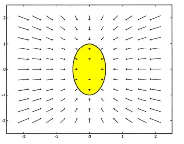
· I I I I

N ·

Figure 2-3: The innermost region (yellow) is B' - the region where the robust stability criterion holds. The white region around it is B1 - the smallest level curve

of the objective function that contains B'. The system is guaranteed to converge to the region B1 and stay within the region.

that case the region B1 may be large.

In the general case, if the error current only bounded, but no other properties of the current are known, global stability cannot be guaranteed. Indeed, as formulated, the error current a injected may be directly sinusoidal, which, given adequately low slope of the original objective function, will translate to sinusoidal oscillations in x. In the case of some specific circuits, however, overall stability may follow from linearity. Specifically, assume that there is some ball B2 around the minimum where

the system can be accurately modeled by the linear approximation. Assume that stability is shown everywhere except a ball B1 around the minimum, as above. Then,

since linear systems are scale invariant, if B2 C B1, this shows stability everywhere.

Note that for this entire argument, the system cannot be underconstrained, or otherwise have a set of more than one minimum. In the case of an underconstrained system, the objective function would only guarantee stability within a subset of the system coordinates; there may be an space in which the system is free to oscillate or saturate.

V

Figure 2-4: Active Transformer. Maintains voltage ratio of V, = 2V,.

For instance, consider a circuit that is intended to hold the constraint V,'= 2V,, as shown in Figure 2-4. It is obvious from this circuit that if it is left unconnected, if the loop gain is just under 1, it will evolve to the solution V, = 2_{V, = 0. If the}

loop gain is more than 1, it will evolve to Vz = 2V, = VRAIL, where, depending on initial conditions, VRAIL is either the positive or negative rail. The constraint is satisfied, but this system behaves in a potentially unstable way within the space where the constraint is satisfied. Chapter 3 shows a context in which this behavior can be exploited to serve a useful function.

2.2.2

Saturation Behavior

In many constraint circuits, saturation behaves as an additional implicit set of con-straints:

Vi : Vee < 1V < Vcc

If this is not the case, additional constraint blocks can prevent the system from reaching saturation behavior. These blocks typically have the form:

Where,Vmin and V,. are some values that guarantee the blocks (both internally and externally) never run into saturation.

2.2.3

High Frequency Stability

In general, there will be some frequency wo (which is independent of the node ca-pacitances), up to which the above logic demonstrates stability directly. For high-frequency stability, it is adequate to make the capacitances on the joint nodes ade-quately large such that the global dynamics dominate. This follows from an argument analogous to, the small-gain theorem.

Informally, consider a linear system. Assume that all of the nodes adjacent to node

j have an error voltage of up to 1Vpp. Calculate the effect of those errors on the current Ij. Chose a node capacitor Cj such that the effect of this current on voltage

Vj is less than 1Vpp. If this is done for all nodes, any high-frequency oscillations will

die off.

More formally, take Ai to be the signal directly injected onto node i from some noise source. Take Bi to be the signal injected onto the node from the adjacent constraint blocks due to voltage variations on both the node and the adjacent nodes. Assume that, for all i, at time t, Ai < a and Bi </p for some constants a and 0. Take a single node j in isolation. Define gij (s) to be the small signal transconductance from node i to node j. Here,

1 1

Bi

E

gij

(Ai + Bi)

<

C8

gij(a+ )

iEAf(j) iEr(j)

Then let:

Then Bj < /3, and maintain the constraint Aj + Bj < a + ,. If this is satisfied for all nodes, the circuit will be high-frequency stable.

Figure 2-5: The circuit holding the constraint 2x = y. All resistors are 10k.

2.3

Test Circuit

A test circuit solved the set of equations:

2x = y

x-y= z

xz+y+z=4

The circuit shown in Figure 2-5 implements first equation, 2x = y. The circuit

shown in Figure 2-6 implements the second equation, x - y = z (or, symmetrically,

x - z = y, y + z = x). Finally, the circuit in shown in Figure 2-7 implements the third

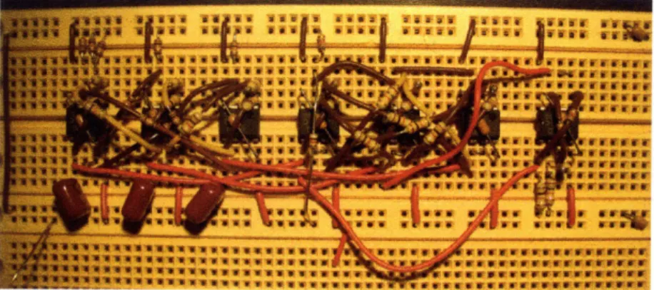
equation, x + y + z = 4. These circuits use the NJM062 operational amplifier, and ±15V rails. All nodes have 0.47pF capacitors on them. A photograph of the circuit is shown in Figure 2-8.

These circuits are more complex than is necessary. It is generally possible to use only one operational amplifier per input. This implementation has more parts than necessary to allow the simple monitoring, instrumentation, and characterization of the circuit and its behavior.

z

y

Figure 2-6: The circuit holding the constraint x - y = z. All resistors are 10k.

Figure 2-7: The circuit holding the constraint x + y + z = 4. All resistors except R3 and R4 are 10k. R3 is 9.1k, while R4 is 1.3k. These were chosen to set the WV node to the appropriate voltage, a given a power supply supply voltage of just under 11V.

Figure 2-8: A photo of the static constraint solving test circuit.

2.3.1

Circuit performance

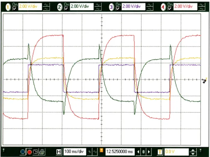
Rate of convergence of the circuit was measured by driving the node labeled 1 with a square wave rather than holding it constant. Scope traces of the results are shown in Figure 2-9, with the mapping of variables to channels and convergence times in Table 2.1.

2.4

_{Simplifying Circuits}

In many cases, circuits designed under this methodology can be further simplified. A complete example of this will be shown in Chapter 4. While many techniques for simplification are specific to each circuit implemented, several common techniques exist. The most common ones are:

1. Common expression elimination. In constraint blocks, it is very common

to calculate the same expression multiple times.

2. Common buffers. In most cases, if several constraint blocks connect to a single node, each will buffer that node voltage internally. All nodes can share a common buffer.

3. Common current output. In many cases, individual constraint blocks use voltage logic, followed by a voltage-to-current stage. In these cases, many

con-2 4 2.00 V/di

Figure 2-9: The scope traces of the dynamics of the static constraint solving circuit. Channel 3 is the input voltage from a function generator, driving the value of the constraint x + y + z = 3_vi,. Channel Channel 1 Channel 2 Channel 3 Channel 4 Convergence Time 27mS 29mS <1mS 42mS Variable x z Vin y

Table 2.1: The convergence times of the static constraint solver test circuit. These were measured as 20% to 80% rise time of the waveforms. Surprisingly, the conver-gence time of channel 4 was substantially slower than channels 1 and 2.

'U@:·':·I;Jl~i `Q ·-.

--2.00 V/div

straint blocks may share an averaging circuit and a common voltage-to-current stage. This is especially useful if the node has controlled gain.

4. Bidirectional-)unidirectional. Some ports interface to external unidirec-tional circuits. These can sometimes be designed as unidirecunidirec-tional, instead of