HAL Id: hal-01959590
https://hal.inria.fr/hal-01959590
Submitted on 18 Dec 2018HAL is a multi-disciplinary open access archive for the deposit and dissemination of sci-entific research documents, whether they are pub-lished or not. The documents may come from teaching and research institutions in France or abroad, or from public or private research centers.
L’archive ouverte pluridisciplinaire HAL, est destinée au dépôt et à la diffusion de documents scientifiques de niveau recherche, publiés ou non, émanant des établissements d’enseignement et de recherche français ou étrangers, des laboratoires publics ou privés.
Applications to Periodic Straight-line Drawings on the
Flat Cylinder and Torus
Luca Castelli Aleardi, Olivier Devillers, Eric Fusy
To cite this version:
Luca Castelli Aleardi, Olivier Devillers, Eric Fusy. Canonical Ordering for Graphs on the Cylinder with Applications to Periodic Straight-line Drawings on the Flat Cylinder and Torus. Journal of Computational Geometry, Carleton University, Computational Geometry Laboratory, 2018, 9 (1), pp.391 - 429. �10.20382/jocg.v9i1a14�. �hal-01959590�
CANONICAL ORDERING FOR GRAPHS ON THE CYLINDER, WITH APPLICATIONS TO PERIODIC STRAIGHT-LINE DRAWINGS ON THE FLAT CYLINDER AND TORUS ∗
Luca Castelli Aleardi,†Olivier Devillers,‡and ´Eric Fusy§
Abstract. We extend the notion of canonical ordering, initially developed for planar tri-angulations and 3-connected planar maps, to cylindric tritri-angulations and more generally to cylindric 3-connected maps. This allows us to extend the incremental straight-line drawing algorithm of de Fraysseix, Pach and Pollack and of Kant from the planar triangulated case and the 3-connected case to this setting. Precisely, for any cylindric essentially 3-connected map G with n vertices, we can obtain in linear time a straight-line drawing of G that is periodic in x-direction, crossing-free, and internally (weakly) convex. The vertices of this drawing lie on a regular grid Z/wZ× [0..h], with w ≤ 2n and h ≤ n(2d + 1), where d is the face-distance between the two boundaries. This also yields an efficient periodic drawing algorithm for graphs on the torus. Precisely, for any essentially 3-connected map G on the torus (i.e., 3-connected in the periodic representation) with n vertices, we can compute in linear time a periodic straight-line drawing of G that is crossing-free and (weakly) convex, on a periodic regular grid Z/wZ× Z/hZ, with w ≤ 2n and h ≤ 1 + 2n(c + 1), where c is the face-width of G. Since c≤√2n, the grid area is O(n5/2).
1 Introduction
The problem of efficiently computing straight-line drawings of planar graphs has attracted a lot of attention over the last two decades. Two combinatorial concepts for planar trian-gulations turn out to be the basis of many classical straight-line drawing algorithms: the canonical ordering (a special ordering of the vertices obtained by a shelling procedure) and the closely related Schnyder wood (a partition of the inner edges of a triangulation into 3 spanning trees with specific incidence conditions). Algorithms based on the canonical ordering [5,10,15,18,20] are typically incremental, adding vertices one by one while keeping the drawing planar. Algorithms based on Schnyder woods [3,14,23] are more global, the (barycentric) coordinates of each vertex have a clear combinatorial meaning (typically the number of faces in certain regions associated to the vertex). Algorithms of both types make it possible to draw in linear time a planar triangulation with n vertices on a grid of size O(n)×O(n). They can also both be extended [14,18] to obtain (weakly) convex drawings of
∗
This work is supported by the ANR grant “EGOS” 12-JS02-002-01 and the ANR grant “GATO” ANR-16-CE40-0009-01. A preliminary version appeared at the 20th International Symposium on Graph Drawing and Network Visualization (GD’12).
†
LIX, ´Ecole Polytechnique, France. http://www.lix.polytechnique.fr/∼amturing/
‡
INRIA Nancy - Grand est, France. www.loria.fr/∼odevil
3-connected maps on a grid of size O(n)× O(n). The problem of obtaining planar drawings of higher genus graphs has been addressed less frequently [9,13,17,19,21,22,24], from both the theoretical and algorithmic point of view. Recently some methods for the straight-line planar drawing of genus g graphs with polynomial grid area O(n3) in the worst case have been described [9,13]. Such methods unfold the graph in the plane along a cut-graph. How-ever, these methods do not yield easily periodic representations: for example, in the case of a torus, the boundary vertices might not be aligned, so that the drawing does not give rise to a periodic drawing. For the torus, a recent article [8] achieves an adaptation of these methods to get alignment of opposite vertices while keeping the size of the periodic grid polynomial, but with the drawback of having a quite large exponent, the guaranteed grid size being O(n4)× O(n4). Another method for drawing toroidal graphs with polyno-mial grid size is the algorithm of Gon¸calves and L´evˆeque [16], which is an adaptation of Schnyder’s drawing principles to the torus1. It achieves both the periodicity requirement
and polynomial grid-size; precisely the size of the periodic regular grid is O(n2)× O(n2) for simple toroidal triangulations (no loops or multiple edges) and is O(n4)× O(n4) for essen-tially simple (simple in the periodic representation) toroidal triangulations. Gon¸calves and L´evˆeque also extend these ideas to 3-connected toroidal maps (similarly, Schnyder woods for plane triangulations have been extended to plane 3-connected maps [14]), but as opposed to the planar case [14], the periodic drawings of 3-connected toroidal maps they obtain do not necessarily have the desired convexity property.
The main contributions of this article are algorithms to obtain crossing-free (weakly) convex straight-line drawings using a small grid-size of essentially 3-connected maps on the cylinder and then on the torus. The key idea here is to adapt the principles of the iterative algorithms based on canonical orderings [15,18] to the cylinder2, first in the case of triangulations, then to the case of 3-connected maps. As in the planar case, the 3-connected case is technically more involved. Precisely, we first adapt the shelling procedure yielding a canonical ordering and the incremental straight-line drawing algorithm of de Fraysseix, Pach, and Pollack [15] (shortly called FPP algorithm thereafter) to triangulations on the cylinder (Section 3). Then, more generally we can also extend the notion of canonical ordering and convex straight-line drawing of Kant [18] to 3-connected maps on the cylinder (Section 4). Precisely, for any essentially internally 3-connected map G on the cylinder, our algorithm yields in linear time a crossing-free internally convex straight-line drawing of G on a regular grid (on the flat cylinder) of the form Z/wZ× [0..h], with w ≤ 2n and h≤ n(2d + 1), where n is the number of vertices of G and d is the face-distance3 between
the two boundaries of G.
Then (in Section 5), we explain how to obtain periodic drawings on the torus by a reduction to the cylindric case using the notion of a tambourine [4]. For any essentially
1Their method relies on the existence of certain orientations where every vertex has outdegree 3. They
have also recently applied these methods to design a bijective encoding scheme for toroidal triangulations [12]. Such technique may induce generalisation to higher genus since it has been proved [1] that a genus g triangulation always admits an orientation where every vertex has for outdegree a non-zero multiple of 3.
2Another notion of canonical ordering for toroidal triangulations has been introduced [7] (this actually
works in any genus and yields an efficient encoding procedure) but we will not use it here.
3The face distance is the smallest possible number of faces traversed by any curve connecting the two
b a d c k i j h g e f b a d c a k i j h e f g
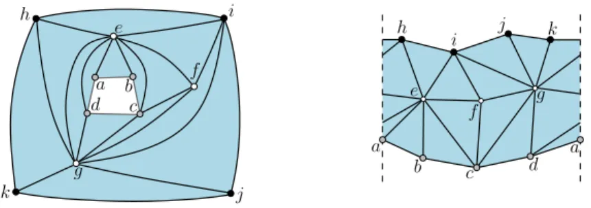
Figure 1: A cylindric triangulation with boundary faces Binn = {a, b, c, d} and Bext = {h, i, j, k}. Left: annular representation. Right: x-periodic representation.
3-connected toroidal map G with n vertices and face-width c (the smallest possible number of points of G met by a non-contractible curve), we can compute in linear time a weakly convex periodic straight-line drawing of G on a regular grid on the flat torus of size w× h, with w≤ 2n and h ≤ 1 + 2n(c + 1). Since c ≤ (2n)1/2 [2], we have h≤ (2n)3/2, so that the grid area is O(n5/2). This improves upon the previously best known grid size for the torus, of O(n2)× O(n2), by Gon¸calves and L´evˆeque [16], and also always gives a weakly convex drawing, which was not guaranteed in [16].
2 Preliminaries
2.1 Graphs embedded on surfaces.
A map of genus g is a connected graph G embedded on the compact orientable surface S of genus g, such that all components of S\G are topological disks, which are called the faces of the map. The map is called planar for g = 0 (embedding on the sphere) and toroidal for g = 1 (embedding on the torus). The dual of a map G is the map G∗ representing the adjacencies of the faces of G, i.e., there is a vertex vf of G∗ in each face f of G, and each edge e of G gives rise to an edge e∗ ={vf, vf0} in G∗, where f and f0 are the faces
on each side of e. A cylindric map is a planar map G with two marked faces Binn and Bext whose boundaries Cinn and Cext are simple cycles (Cinnand Cext might share vertices and edges). The faces Binn and Bext are respectively called the inner boundary-face and the outer boundary-face (we will often consider cylindric maps in the annular representation where Bextis the outer face, as shown in Fig.1left-part). The other faces are called internal faces. Boundary vertices and edges are those belonging to Cinn (gray circles in Fig. 1) or Cext (black circles in Fig. 1); the other ones are called internal vertices (white circles in Fig. 1) and edges. The notations G, Binn, Bext, Cinn, Cext will be used throughout the article.
2.2 Periodic drawings.
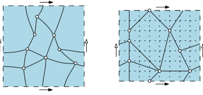
Here we consider the problem of drawing a cylindric map on the flat cylinder and drawing a toroidal map on the flat torus. For w > 0 and h > 0, the flat cylinder of width w and
Figure 2: Left: an essentially 3-connected toroidal map G. Right: a weakly convex straight-line drawing of G on a periodic regular grid of size 8× 7.
height h is the rectangle [0, w]× [0, h] where the vertical sides are identified. A point on this cylinder is located by two coordinates x∈ R/wZ and y ∈ [0, h]. The flat torus of width w and height h is the rectangle [0, w]× [0, h] where both pairs of opposite sides are identified. A point on this torus is located by two coordinates x ∈ R/wZ and y ∈ R/hZ. Assume from now on that w and h are positive integers. For a cylindric map G, a periodic straight-line drawing of G of width w and height h is a crossing-free straight-line drawing (edges are drawn as segments, two edges can meet only at common end-points) of G on the flat cylinder of width w and height h, such that the vertex-coordinates are in Z/wZ× [0..h].Similarly, for a toroidal map G, a periodic straight-line drawing of G of width w and height h is a crossing-free straight-line drawing (edges are drawn as segments, two edges can meet only at common end-points) of G on the flat torus of width w and height h, such that the vertex-coordinates are in Z/wZ× Z/hZ.A periodic straight-line drawing on the flat torus is said to be weakly convex if all corners have angle at most π, see Fig. 2 for an example. Note that a drawing of a toroidal triangulation is automatically weakly convex, so that convexity becomes a constraint only when there are faces of degree larger than 3.
3 Periodic drawings of cylindric triangulations
In this section we describe an algorithm to obtain periodic (in x) drawings of cylindric triangulations. We extend these results to 3-connected maps on the cylinder in Section 4. We start with the case of triangulated maps for pedagogical reasons: the different steps are the same as the ones to be used in the more general 3-connected case; but the arguments at each step are simpler in the triangulated case.
3.1 De nitions and statement of the result
A cylindric triangulation is a cylindric map T such that all internal faces are triangles. A cylindric map is called simple if it has no loops nor multiple edges, and is called essentially simple if it has no loops nor multiple edges in the periodic representation. Note that an essentially simple cylindric map might have 2-cycles and 1-cycles (loops), which have to be
non-contractible (they have Binn on one side and Bext on the other side), and two loops cannot be incident to the same vertex. We also define a chordal edge, or chord, at Cinn as an edge not on Cinn but with its two ends on Cinn. Similarly a chord at Cext is an edge not on Cext but with its two ends on Cext. For a cylindric map, the edge-distance d between the two boundaries is the length of a shortest possible path starting from a vertex of Cinn and ending at a vertex of Cext (possibly d = 0). The main result obtained in this section is the following:
Theorem 1. For each essentially simple cylindric triangulationG, one can compute in lin-ear time a crossing-free straight-line drawing ofG on an x-periodic regular grid Z/wZ×[0, h], where —withn the number of vertices and d the edge-distance between the two boundaries— w ≤ 2n and h ≤ 2n(d + 1). In the drawing, the upper (resp. lower) boundary is a broken line monotone in x, formed by segments of slope at most 1 in absolute value.
As a first step we will restrict to the case with no chordal edge at Cinn:
Proposition 2. For each essentially simple cylindric triangulationG with no chordal edge at Cinn, one can compute in linear time a crossing-free straight-line drawing of G on an x-periodic regular grid Z/wZ× [0..h] where —with n the number of vertices of G and d the edge-distance between the two boundaries— w≤ 2n and h ≤ n(2d + 1), such that the upper boundary is a broken line monotone in x formed by segments of slope in {+1, −1, 0} and the lower boundary is an horizontal line.
To prove Proposition2 we will start with the subcase of cylindric simple triangula-tions. In that case we will introduce a notion of canonical ordering (where it is necessary that Cinn has no chordal edge). This makes it possible to design an incremental periodic drawing algorithm, which can be seen as the cylindric counterpart of the FPP algorithm. Then we will extend the canonical ordering and periodic drawing algorithm to cylindric essentially simple triangulations with no loop. We will then explain how to deal with non-contractible loops. This will establish Proposition 2. Finally Proposition 2 and handling chordal edges at Cinn will yield Theorem 1as explained in Section 3.6.
3.2 Canonical ordering for cylindric simple triangulations with no chord at Cinn. We first introduce a notion of canonical ordering (classically studied on plane graphs) for cylindric simple triangulations:
Definition 3. Let G be a cylindric simple triangulation with no chordal edge at Cinn. An ordering π = {v1, v2, . . . , vn} of the vertices of G\Cinn is called a canonical ordering if it satisfies:
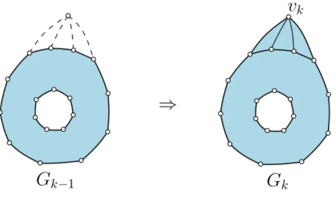
• For each k ∈ [0..n] the map Gk induced by Cinn and by the vertices {v1, . . . , vk} is a cylindric triangulation. The outer boundary-face of Gk is denoted Ck.
• For each k ∈ [1..n], the vertex vk is on Ck, and its neighbours in Gk−1 are consecutive on Ck−1 (see Fig.3).
⇒
G
k−1G
kv
kFigure 3: From Gk−1 to Gk in a canonical ordering for a cylindric simple triangulation (annular representation, only the boundaries and next added vertex and added edges are shown).
The notion of canonical ordering makes it possible to construct a cylindric triangu-lation G incrementally, starting from G0= Cinnand adding one vertex at each step. This is similar to canonical orderings for planar triangulations, as introduced by de Fraysseix, Pach and Pollack [15]; the main difference is that, for a planar triangulation, one starts with G0 being an edge, whereas here one starts with G0 being a cycle, seen as a cylindric map with no internal face.
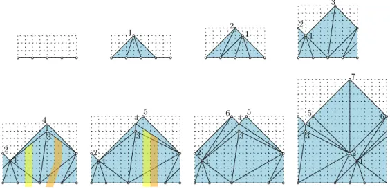
The computation of such an ordering is done by a shelling procedure similar to the one considered in the planar case [6,15]. At each step the graph formed by the remaining vertices is a cylindric triangulation, the inner boundary remains Cinn all the way, while the outer boundary (initially Cext) has its contour, denoted by Ck, getting closer to Cinn. A vertex v ∈ Ck is free if v is incident to no chord of Ck and if v /∈ Cinn. The shelling procedure goes as follows, with n the number of vertices in G\Cinn:
for k from n to 1, choose a free vertex v on Ck, assign vk ← v, and then delete v together with all its incident edges.
The existence of a free vertex at each step follows from the same argument as in the planar case [6]. First, since there is no chord at Cinn, then as long as Ck 6= Cinn there is at least one vertex on Ck\Cinn. If there is no chord for Ck, then any vertex v∈ Ck\Cinn is free. If there is at least one chord e ={u, v} for Ck, let Pe be the path connecting u and v on Ck such that the cycle Pe+ e does not enclose the inner boundary-face in the annular representation, and let de be the length of Pe (note that de≥ 2). Let e = {u, v} be a chord such that de is smallest possible. Then any vertex in Pe\{u, v} is free. Since there exists a free vertex at each step, the procedure terminates. Let us now justify that the shelling procedure has linear time complexity. Note that an outer vertex v ∈ Ck\Cinn is free if and only if the number N (v) of neighbours of v belonging to Ck is equal to two. So we just have to mark the vertices when they become outer vertices of the current triangulation and maintain N (v) for these outer vertices. Notice that when v become an outer vertex, it remains an outer vertex and its value N (v) can only decrease. The free vertices (those
7 7 6 7 6 5 7 6 5 4 7 6 5 4 3 7 6 5 4 3 2 7 6 5 4 3 2 1 w1 w2 w2 w2 w2 edge of F
Figure 4: Shelling procedure to compute a canonical ordering of a cylindric simple tri-angulation (at each step the next shelled vertex is surrounded). The underlying forest is computed on the fly; the last drawing shows the underlying forest superimposed with the dual forest. The graph is the one of Fig. 1.
for which N (v) = 2) are put in a buffer, picking any element of the buffer at each step. All this can be done in time O(|E|), with |E| ≤ 3n the number of edges of the cylindric triangulation. To sum up:
Proposition 4. Any cylindric simple triangulation G with no chordal edge at Cinn admits a canonical ordering that can be computed in linear time by a shelling procedure.
Underlying forest and dual forest. Given a cylindric simple triangulation G with no chordal edge at Cinnendowed with a canonical ordering π, we define the underlying forest F for π as the oriented subgraph of G where each vertex v∈ Cext has outdegree 0, and where each v /∈ Cext has exactly one outgoing edge, which is connected to the adjacent vertex u of v of largest label in π. The forest F can be computed on the fly during the shelling procedure: when processing an admissible vertex vk, for each neighbour v of vk such that
v /∈ Ck, add the edge {v, vk} to F , and orient it from v to vk. Since the edges are oriented in increasing labels, F is an oriented forest; it spans all vertices of G and has its roots on Cext. The augmented map G (“ G has to be seen as a map on the sphere) is obtained from“
G by adding a vertex w1 inside Binn, a vertex w2 inside Bext, and connecting all vertices around Binn to w1 and all vertices around Bext to w2, thus triangulating the interiors of Binn and Bext. We denote by F the forest F plus all edges incident to w“ 1 and all edges
incident to w2. The dual forest F∗ for π is defined as the graph formed by the vertices of
“
G∗ (the dual of G) and by the edges of“ G“∗ that are dual to edges not in F . Since“ F is a“
spanning connected subgraph of G, F“ ∗ is a spanning forest of G“∗. Precisely, each of the
trees (connected components) of F∗ is rooted at a vertex “in front of” each edge of Cinn, and the edges of the tree can be oriented toward this root-vertex, see Fig. 4bottom right. Each edge e∗ of F∗ is in a certain tree-component T∗ rooted at a vertex v0 in front of a certain edge of Cinn. Let P be the path from e∗ to v0 in T∗; P is shortly called the root-path of e∗.
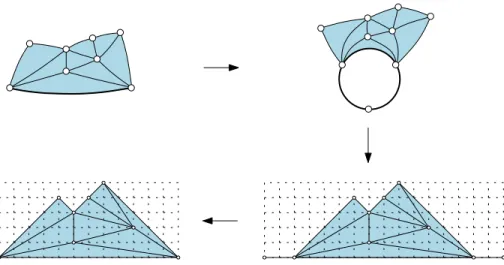
3.3 Periodic drawing algorithm for cylindric simple triangulations, no chord at Cinn. Given a cylindric simple triangulation G with no chord at Cinn, we first compute a canonical ordering of G, and then draw G in an incremental way. We start with a cylinder of width 2|Cinn| and height 0 (i.e., a circle of length 2|Cinn|) and draw the vertices of Cinn equally spaced on the circle: space 2 between two consecutive vertices4.
Then the strategy for each k ≥ 1 is to compute the drawing of Gkout of the drawing of Gk−1. Note that the set of vertices of Ck−1 that are neighbours of vk forms a path γ on Ck−1. Traversing γ with the outer face of Gk−1 to the left, let e` be the first edge of γ and er be the last edge of γ (note that e` = er if vk has only two neighbours on Ck−1). Let also ak be the starting vertex and let bk be the ending vertex of γ. Two cases can occur.
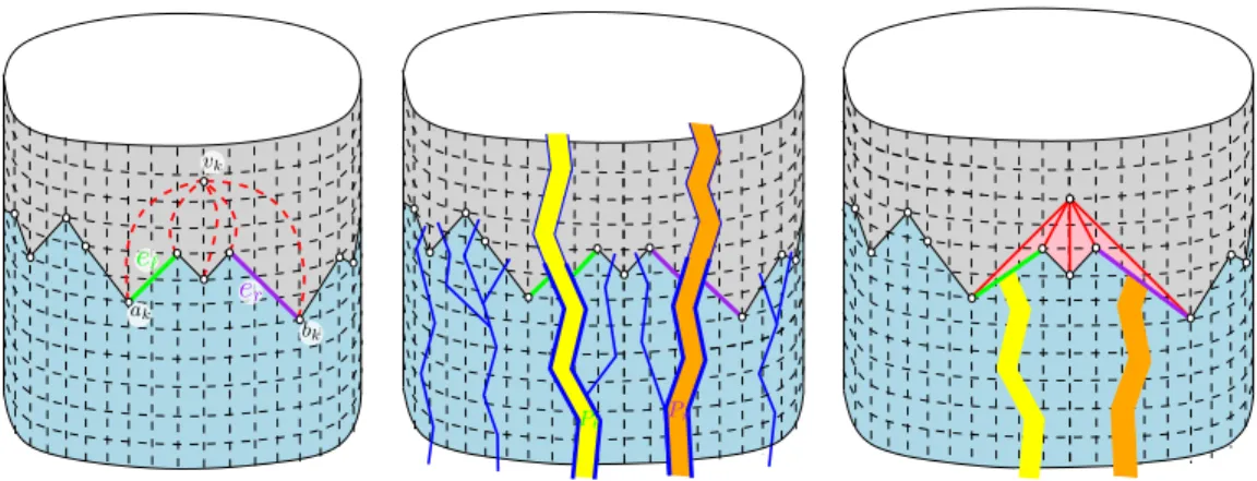
(1) If, in the drawing of Gk−1 obtained so far, slope(e`) < 1 and slope(er) > −1, then we can directly insert vk in the drawing. We place vk at the intersection of the ray of slope 1 starting from ak and the ray of slope −1 starting from bk, and we connect vk to all vertices of γ by segments.
(2) If slope(e`) = 1 or slope(er) =−1, then we cannot directly insert vk as done in Case (1), because the edges e` and {ak, vk} would overlap if slope(e`) = 1, or the edges er and{bk, vk} would overlap if slope(er) =−1. We first have to perform stretching operations (thereby increasing the cylinder width by 2) to make the slopes of e` and er smaller than 1 in absolute value. Define the x-span of an edge e in the cylindric drawing as the number of columns [i, i + 1]× [0, +∞) that meet the interior of e (we have no need for a more complicated definition since, in our drawings, a column will never meet an edge more than once). Consider the dual forest F∗ for the canonical ordering restricted to Gk−1. Let P` (resp. Pr) be the root-path of e∗` (resp. e∗r) in F∗. We stretch the cylinder by inserting a vertical strip of length 1 along P` and another along Pr, see Fig. 5. This comes down to
4It is also possible to start with any configuration of points on a circle such that any two consecutive
P` Pr ak bk er e` vk
Figure 5: One step of the incremental drawing algorithm. Two vertical strips of width 1 (each one along a path in the dual forest) are inserted in order to make the slopes of e` and er smaller than 1 in absolute value. Then the new vertex and its edges connected to the upper boundary can be drawn in a planar way.
increasing by 1 the x-span of each edge of Gk−1 dual to an edge in P`, and then increasing by 1 the x-span of each edge dual to an edge in Pr (note that P` and Pr are not necessarily disjoint, in which case the x-span of an edge dual to an edge in P`∩ Pr is increased by 2). After these stretching operations,5 whose effect is to make the slopes of e` and er strictly smaller than 1 in absolute value, we insert, as in Case (1), the vertex vk at the intersection of the ray of slope 1 starting from ak and the ray of slope −1 starting from bk, and we connect vk to all vertices of γ by segments.
Note that in the two cases (1) and (2), the two rays from akand bkactually intersect at a grid point since the Manhattan distance between any two vertices on Ck−1 is even. Fig.6 shows the execution of the algorithm on the example of Fig. 4.
The fact that the drawing remains crossing-free relies on the fact that all edges of the upper boundary have slope at most 1 in absolute value, and on the following inductive property (similar to the one used in [15]), which is easily shown to be maintained at each step k from 1 to n:
Pl: for each edge e on Ck (the upper boundary of Gk), let Pe be the root-path of e∗ in F∗, let Ee be the set of edges dual to edges in Pe, and let δe be any nonnegative integer. Then the drawing remains crossing-free after successively increasing by δethe x-span of all edges of Ee, for all e∈ Ck.
We now prove the bounds on the grid-size, where we call w the width and h the
5In the FPP algorithm for planar triangulations, the step to make the (absolute value of) slopes of e `and
er smaller than 1 is formulated as a shift of certain subgraphs described in terms of the underlying forest
F. The extension of this formulation to the cylinder would be quite cumbersome. We find the alternative formulation with strip insertions more convenient for the cylinder. In addition it also gives rise to a very easy linear-time algorithm (another linear-time version of the FPP algorithm is given in [11]).
1 2 1 2 1 3 1 2 3 4 6 4 5 2 1 3 5 4 6 2 1 3 7 5 4 2 1 3
Figure 6: Complete execution of the algorithm computing an x-periodic drawing of a cylin-dric simple triangulation with no chordal edge at Binn. The vertices are processed in in-creasing label (the canonical ordering is the one computed in Fig.4).
height of the cylinder on which G is drawn. If|Cinn| = t then the initial cylinder is 2t×0; and at each vertex insertion, the grid-width grows by 0 or 2. Hence w≤ 2n. In addition, due to the slope conditions (slopes of boundary-edges are at most 1 in absolute value), the vertical span of every edge e is not larger than the current width at the time when e is inserted in the drawing. Hence, if we denote by v the vertex of Cext that is closest (at distance d) from Cinn, then the ordinate of v is at most d· (2n). And due to the slope conditions, the vertical span of Cext in the drawing is at most w/2≤ n. Hence the grid-height is at most n(2d + 1). The linear-time complexity is shown next.
Linear-time complexity. An important remark is that, instead of computing the x-coordinates and y-x-coordinates of vertices in the drawing, one can compute the y-x-coordinates of vertices and the x-span of edges (as well as the knowledge of which extremity of the edge is the left-end vertex and which extremity is the right-end vertex). In a first pass, for k from 1 to n, one computes the y-coordinates of vertices and the x-span re of each edge e ∈ G at the time t = k when it appears on Gk (as well one gets to know which extremity of e is the left-end vertex). Afterwards if e /∈ F , the x-span of e might further increase due to insertion of new vertices; let se be the total further increase undergone by e. Note that for each edge e not in F , if e /∈ Cext there is a certain step k such that e∈ Ck−1 and e /∈ Ck. Let we ∈ {0, 1, 2} be defined as the stretch (increase of x-span) that e undergoes just before adding vk to the drawing; in case e∈ Cext no such step k exists and we assign we= 0. We call we the weight of e (the quantities wecan be computed in a first pass, together with the quantities re). Let P be the root-path of e∗. When stretching e just before adding vk, all edges dual to edges of P undergo the same stretch, by we. In other words, if we denote by Te∗ the subtree of F∗ hanging from e∗ (including e∗), and denote by We the total weight of the dual of the edges in Te∗, then se = We. Hence the total x-span of each edge e ∈ G is
Figure 7: The FPP algorithm for simple planar quasi-triangulations is recovered from our algorithm by adding a vertex of degree 2 to complete the inner boundary.
given by re+ se, where se= 0 if e∈ F or e ∈ Cext, and se= Weif e /∈ F and e /∈ Cext. Since all quantities secan easily be computed in linear time from the quantities we, starting from the leaves and going up to the roots of F∗, this gives a linear-time algorithm.
To sum up, we have proved Proposition 2 for cylindric simple triangulations with no chord at Cinn.
Remark 5. For each edge e of Cinn, let rebe the initial horizontal stretch of e in the drawing procedure (an even number, classically re = 2 to have a compact drawing). And let te be the final horizontal stretch in the drawing procedure. The vectors R = (re)e∈Cinn and
T = (te)e∈Cinn are called initial-stretch and final-stretch vectors relative to the drawing of
G (endowed with a given canonical ordering). Then the vector S := T − R is an invariant, it does not depend on R since se = te− re just depends on the underlying forest and dual forest given by the canonical ordering. Hence, if with R as initial stretch-vector we obtain a drawing with final-stretch vector T , then for any vector T0 of the form T + 2V —with V a vector of non-negative integers— we can obtain a drawing with final-stretch vector T0, by taking R0 = R + 2V as initial-stretch vector instead of R.
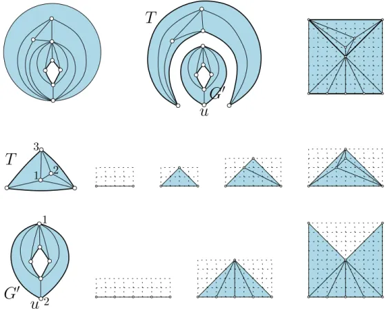
Remark 6. Note that our algorithm can be seen as an extension of the FPP algorithm, which works for simple planar quasi-triangulations, i.e., simple graphs embedded in the plane with triangular inner faces and a polygonal outer face. If we are given a simple planar quasi-triangulation Q, we can turn it into a cylindric simple triangulation G by adding a vertex of degree 2 connected to the two ends of the root-edge. Then the FPP drawing of Q is recovered from the periodic drawing of Q upon deleting the added vertex, see Fig.7.
3.4 Allowing for non-contractible 2-cycles (no chord at Cinn).
⇒
Gk−1 Gk
vk
Figure 8: When 2-cycles are allowed, the additional case shown here can occur for the transition from Gk−1 to Gk.
extended to essentially simple cylindric triangulations with no loop but possibly with non-contractible 2-cycles. Let G be such a cylindric map with no chord at Cinn. The definition of canonical ordering for G is exactly the same as for simple cylindric triangulations, adding the possibility that Gk is obtained from Gk−1 as shown in Fig.8. Such a canonical ordering can be computed by a shelling procedure that extends the one of Section3.2. A 2-cycle is called internal if its two incident vertices are not both on the outer boundary. This time, a vertex on the outer boundary and not on the inner boundary is called free if it is not incident to a chord nor incident to an internal 2-cycle.
The shelling procedure consists in choosing a free vertex at each step, and deleting it together with its incident edges, until there just remains the inner boundary. The existence of a free vertex, when the cylindric map is not reduced to a cycle, is proved as follows. First, since there is no chord at Cinn, as long as Cext6= Cinn there is at least one vertex on Cext\Cinn. If there is no chord nor internal 2-cycle incident to a vertex on Cext, then any vertex on Cext\Cinn is free. If there is at least one chord at Cext, for each chord e at Cext let Pe be the path on Cext such that P + e does not enclose Binn, and let de be the length of Pe. Let e ={u, v} be a chord at Cext such that de is smallest possible. Then any vertex v ∈ Pe\{u, v} is admissible. If there is no chord but there is at least one internal 2-cycle, consider the largest internal 2-cycle (in terms of containment, noticing that the 2-cycles are nested in the annular representation). Since there is no chord at Cinn, at least one outer vertex v is strictly exterior to this 2-cycle, hence is free.
A linear time algorithm is also readily obtained by maintaining, for each outer vertex, how many neighbours on Cext it has and how many internal 2-chords it is incident to. Note that such a canonical ordering also induces an underlying forest F and the dual forest F∗. These can be computed on the fly during the shelling procedure, in the same way as for simple cylindric triangulations. Finally, the incremental drawing algorithm (and linear complexity using the dual forest) works exactly in the same way as for cylindric simple triangulations. An example is shown in Fig. 9. The grid bounds are also the same as for simple triangulations (the arguments to obtain the bounds in the simple case did not use the fact that there are no 2-cycles). So this gives Proposition 2 for essentially simple triangulations with no loops. Finally, note that Remark 5 still holds here (the arguments are the same).
4 4 3 4 3 2 4 3 2 1 1 12 2 1 3 3 2 1 4
Figure 9: Left-side: the shelling procedure for an essentially simple loopless cylindric tri-angulation G with no chord at Cinn; the last drawing shows the underlying forest and dual forest. Right-side: the incremental drawing algorithm.
2 3 1 1 4 12 1 2 3 2 4 3 1
Figure 10: Drawing algorithm when the inner boundary is the unique loop.
3.5 Allowing for non-contractible loops (no chord at Cinn).
We finally explain how to deal with non-contractible loops. Our strategy is not to extend the notion of canonical ordering but simply to decompose (at the loops, which are nested) such a cylindric map into a “tower” of components, where the only loops in each component are at the boundary-faces. Let G be an essentially simple cylindric triangulation with n vertices and at least one loop. There are a few cases to consider:
(a)Cinnis the unique loop ofG. In that case, the algorithm of Section3.2(canonical ordering, shelling procedure, and incremental drawing procedure) works in the same way, see Fig. 10 for an example. Let 2m be the width of the drawing. By the arguments of Remark 5, for any m0 ≥ m, G has a periodic drawing of width 2m0 and height at most m0(2d + 1), with d the edge-distance between the two boundaries.
(b)Cext is a loop, Cinn is possibly a loop, and there are no other loops. Assume Cext is a loop and G is not reduced to that loop (i.e., Cext 6= Cinn). Let u be the vertex incident to the loop (note that u is not on Cinn since there is no chord at Cinn), and let c be the innermost 2-cycle incident to u. Cutting along c (see Fig.11), we obtain two components: a
3 2 1 2 1
T
G
0G
0T
u
u
Figure 11: Drawing algorithm when the outer face contour is a loop (and there is no other loop except possibly at Cinn): the map is split along the innermost 2-cycle (the initial x-span of T is taken to be 4 instead of 2 so that the drawings of Q and G0 fit together).
planar triangulation T and a cylindric essentially simple triangulation G0 such that: G0 has no loop except possibly at Cinn, G0 has outer degree 2 and u is a free vertex for G0. Hence there is a canonical ordering for G0 such that u is the first shelled vertex. Take a periodic drawing of G0 for this canonical ordering and take an FPP drawing of T . The widths of the respective drawings are even numbers, denoted 2n1 and 2n2. Let m = max(n1, n2). By the arguments of Remark 5 it is possible to redraw the graph that has the smaller grid-width so that it gets width 2m, after which both drawings are of width 2m. Then the drawing of T (taken upside down) fits into the upper boundary of G0 yielding a periodic drawing of G of width 2m, see Fig. 11. The height of the drawing is at most 2dm≤ 2dn, where d is the edge-distance between the two boundaries (indeed, in the usual bound h≤ (2d + 1)m, the +1 in the parenthesis is due to the vertical extension of the upper boundary, which is 0 here).
(c) General case (with no chord at Cinn). We can assume there is at least one loop (the case with no loop has been covered in the last section). Let `1, . . . , `r be the sequence of nested loops of G, with `1 the innermost loop and `r the outermost loop; and let G(0), . . . , G(r) be the r + 1 components that result from cutting successively along all
Figure 12: Drawing an essentially simple triangulation G (no chord at Cinn); G is first decomposed at its loops; each component is drawn so that the component-drawings have the same width, and can be stacked up to obtain a periodic drawing of G.
these loops. For i∈ [0..r] let di be the edge-distance between the two boundaries in G(i); and let d be the edge-distance between the two boundaries of G. Note that d = P
idi. Each component Gi has loops only at the boundary-face contours, hence has a periodic drawing (according to cases (a) and (b)) such that boundaries that are loops are drawn as horizontal lines. Let 2n1, . . . , 2nr be the widths of the drawings of G(1), . . . , G(r) thus obtained. Let m = max(n1, . . . , nr). By the arguments of Remark 5, each of the graphs G(i) can be redrawn so as to have width 2m. Stacking up all these drawings we obtain a periodic drawing of G of width 2m, see Fig.12. Regarding the grid size, the width is 2m, with clearly m≤ n, and the height of the drawing of Gi is at most 2mdi for i ∈ [0..r − 1] and at most m(2dr+ 1) for i = r. Hence the total height is at most m(2d + 1)≤ n(2d + 1). This establishes Proposition 2.
3.6 Allowing for chords at Cinn.
We finally explain how to draw a cylindric essentially simple triangulation when allowing for chords incident to Cinn. It is good to view Bextas the top boundary-face and Binnas the bottom boundary face, and imagine a standing cylinder. For each chord e at the cycle Cinn, the component under e, denoted Qe, is the face-connected part of G that lies below e; such a component is a quasi-triangulation (polygonal outer face, triangular inner faces) rooted at the edge e. A chordal edge e of Cinnis maximal if the component Qeunder e is not strictly included in the component under another chord at Cinn. The FPP-size |e| of such an edge e is defined as the width of the FPP drawing of Qe. If we delete the component under each maximal chordal edge (i.e., delete everything from the component except for the chordal
e e
e
e
Figure 13: Drawing a cylindric triangulation with chords at Cinn (the top-line example is simple, the bottom-line example is essentially simple with loops and 2-cycles in the annular representation). In the top-line example, to make enough space to place the component under e, one takes 6 (instead of 2) as the initial x-span of e. In the bottom-line example, to make enough space to place the component under e, one takes 4 (instead of 2) as the initial x-span of e.
edge itself) we get a new bottom cycle C00 that is chordless, so we can draw the reduced cylindric triangulation G0 using the algorithm of Proposition2. Let webe the width of each edge e of C00 in this drawing. According to Remark5, we can redraw G0 such that each edge e∈ C00 that is chordal in G has width `(e), with `(e) defined as the smallest integer that is at least max(we,|e|) and such that `(e) − we is even (note that `(e)≤ max(we,|e| + 1)).
Then for each maximal chord e of C0, we draw the component Qe under e using the FPP algorithm. This drawing has width|e|, with e as horizontal bottom edge of length |e| and with the other outer edges of slopes in ±1. We shift the left-extremity of e to the left so that the drawing of Qegets width `(e), then we rotate the drawing of Qe by 180 degrees and plug it into the drawing of G0, see Fig. 13. The overall drawing of G is clearly planar. We now give bounds on the grid-size of the overall drawing. Let S be the sum of the FPP-sizes over all maximal chords e at Cinn, and let n0 be the number of vertices of G0. Clearly the width w of the drawing of G satisfies w≤ 2n0+P
e∈C0
0`(e)− we≤ 2n
0+ S. For each maximal chord e at Cinnlet ne+ 2 be the number of vertices of the component Qe under e. Let N be the sum of the quantities ne over all maximal chords at Cinn, so that n = n0+ N . Since the FPP drawing of a quasi-triangulation with p≥ 3 vertices has width at most 2p− 4, we have |e| ≤ 2ne for each maximal chord at Cinn. Hence S≤ 2N, so that w≤ 2n. Regarding the height of the drawing, by the same arguments as in Section3.3, the height of the drawing of G0 is at most n(2d + 1), with d the edge-distance between the two
Figure 14: Left: a cylindric map G with a (contractible) 1-separating curve and a (non-contractible and nondegenerate) 2-separating curve (in bold line). Right: a cylindric map with a contractible degenerate 2-separating curve (the enclosed area appears in yellow).
boundaries. After adding the components under the chords at Cinn, the lower boundary is not horizontal anymore, but since it is made of segments of slope at most 1 in absolute value, it has vertical extension at most w/2 ≤ n. Hence the overall height of the drawing is at most n(2d + 1) + n = 2n(d + 1). This finally yields the result pursued in this section, Theorem1.
4 Periodic drawing of 3-connected maps on the cylinder
We now extend the results obtained in Section3to the more general 3-connected case. The approach is completely parallel to the one used in Section3, but the arguments at each step are more technical.
4.1 De nitions and statement of the result
Let G be a cylindric map, embedded in the plane using the annular representation (with Bext as the outer face and Binn as the marked inner face). We define a 1-separating curve as a closed curve γ not meeting any edge and intersecting G in exactly one vertex, the unique visited face being an internal face, and such that the area enclosed by γ contains at least one edge. Such a curve γ is called non-contractible if the area enclosed by γ entirely contains Binn. We now define a 2-separating curve as a closed curve γ intersecting G in two vertices (not meeting any edge), visiting exactly two faces, and such that the area enclosed by γ strictly contains at least one vertex; again γ is said to be non-contractible if it entirely encloses Binn. We also allow for the degenerate situation of a contractible 2-separating curve where the two incident vertices are equal (it is still required that the enclosed area strictly contains at least one vertex), see Fig. 14 for an example. Two 1-separating curves (resp. two 2-separating curves) are considered as equivalent if they are isotopic. It is convenient —and will always be assumed from now on— to discard non-contractible curves passing by the outer face.
We consider in this section certain cylindric maps G with some marked vertices on Cext and some marked vertices on Cinn which are called active (if a vertex is on Cinn∩ Cext
it might be active for Cinnor Cext, or both, or none). As we will see, when all active vertices are for Cext, these vertices are to be the ones that are allowed to be selected during the shelling procedures to compute a canonical ordering in the more general 3-connected case presented here. The terminology of active vertices will also be useful when presenting the drawing algorithm for toroidal 3-connected maps via a reduction to the cylindric case (we will delete certain edges of the toroidal map to make it a cylindric map, and declare as active the vertices of the cylindric map incident to at least one deleted edge).
A cylindric map G with some active vertices is called internally 3-connected if is has no 1-separating curve, and any 2-separating curve is contractible (and nondegenerate) and strictly encloses at least one active vertex (see Fig. 17(a) for an example). And G is called essentially internally 3-connected if there is no contractible 1-separating curve, and any contractible 2-separating curve (possibly degenerate) strictly encloses at least one active vertex. Being essentially internally 3-connected can also be conveniently characterized in the x-periodic representation ˆG of G: a 1-separating (resp. 2-separating) curve in ˆG is a simple closed curve not meeting any edge of ˆG, meeting ˆG at exactly 1 vertex (resp. 2 vertices), and whose interior strictly contains at least one vertex. Then G is essentially internally 3-connected if and only if, in ˆG, there is no 1-separating curve and any 2-separating curve strictly encloses at least one active vertex.
For a cylindric map G with active vertices, a periodic straight-line drawing of G is called weakly convex if all corners have angle at most π, except possibly for corners of Binn (resp. Bext) at an active vertex for Cinn(resp. for Cext), whose angle in the drawing can be larger than π. For a cylindric map G, the face-distance between the two boundaries is the minimal possible integer q such that there is a curve in G starting from a vertex of Cinn, ending at a vertex of Cext, not meeting any edge, and passing by q (internal) faces of G. The main result obtained in this section is the following:
Theorem 7. For each essentially internally 3-connected cylindric map G with at least one active vertex, one can compute in linear time a periodic weakly convex drawing of G on an x-periodic regular grid Z/wZ× [0, h], where —with n the number of vertices and d the face-distance between the two boundaries— w≤ 2n and h ≤ 2n(d + 1). In the drawing, the upper (resp. lower) boundary is a broken line monotone in x formed by segments of slope at most1 in absolute value.
Having a convexity condition (angle at most π) at all corners except possibly at the active vertices is important in view of our drawing algorithm for toroidal 3-connected maps. Indeed, we will obtain a convex periodic toroidal drawing by adding edges to a periodic cylindric drawing, and the corners not at active vertices will be the ones kept unchanged (not receiving any additional edge), it is thus necessary that these have angle at most π already in the cylindric drawing.
As a first step to show Theorem 7, we will prove the result when there is no active vertex on Cinn:
Proposition 8. For each essentially internally 3-connected cylindric map G where Cext has at least one active vertex and Cinn has no active vertex, one can compute in linear time a periodic weakly convex drawing of G on an x-periodic regular grid Z/wZ× [0, h],
where —withn the number of vertices and d the face-distance between the two boundaries— w≤ 2n and h ≤ n(2d + 1). In the drawing, the upper boundary is a broken line, monotone in x, formed by segments of slope at most 1 in absolute value, and the lower boundary is an horizontal line.
Note that Theorem 7 and Proposition 8 are respectively extensions of Theorem 1
and Proposition 2. Indeed, for an essentially simple cylindric triangulation G, making all boundary-vertices of G active yields an essentially internally 3-connected cylindric map, and if G has no chord at Cinn, then making all vertices of Cext active yields an essentially internally 3-connected cylindric map with no active vertex at Cinn. In addition, for an essen-tially simple cylindric triangulation, the face-distance between the two boundaries coincides with the edge-distance between the two boundaries. To prove Proposition8(the strategy is parallel to the one we have followed to prove Proposition2 for cylindric triangulations) we will start with the subcase where G is internally 3-connected. In that case we will introduce a notion of canonical ordering, which extends both the canonical ordering for cylindric tri-angulations introduced in Section3.2, and the canonical ordering for internally 3-connected plane graphs introduced by Kant [18]. This makes it possible to design an incremental periodic drawing algorithm, which is the cylindric counterpart of the algorithm introduced by Kant [18] in the planar case (which itself extends the FPP algorithm to 3-connected planar maps). Then we will extend the canonical ordering and drawing algorithm to the subcase where there is no 1-separating curve; after which we will explain how to deal with 1-separating curves. This will establish Proposition 8. We will then explain how to deal with active vertices at Cinn. This will yield Theorem 7.
4.2 Restatement of the de nitions in terms of the corner-map
We provide here a classical reformulation of the 3-connectedness conditions in terms of the so-called corner-map, which provides a more combinatorial way of viewing 2-separating curves. Given a cylindric map G (whose vertices are considered as white), in its annular representation, the corner-map S of G is obtained by inserting a black vertex vf in each internal face f of G and connecting vf to all the corners around f ; S is the graph made of black and white vertices and of the (newly added) edges between black and white vertices. The completed mapG of G is defined as G superimposed with S (see Fig.“ 15for an example).
A separating 4-cycle in S is a 4-cycle containing at least one vertex in its interior; it is called non-contractible if it completely encloses Binn and contractible otherwise. Note that a separating 4-cycle exactly corresponds to a separating 2-curve of G passing by two internal faces. We define (in G) a 2-chord γ for C“ ext as a path e1, e2 of length two in S starting
from a vertex u of Cext and ending at a vertex v 6= u of Cext. We denote by Pγ the path from u to v on Cext such that the cycle Cγ := Pγ ∪ γ does not contain Binn; Cγ is called the cycle enclosed by the 2-chord. The 2-chord γ is called separating if Pγ is of length larger than 1, i.e., has at least one non-extremal vertex. The non-extremal vertices of Pγ are said to be enclosed by γ. A 2-chord or separating 2-chord at Cinn is defined analogously. Note that a separating 2-chord at Cext (resp. at Cinn) exactly corresponds to a 2-separating curve of G passing by Bext and by an internal face (resp. passing by Binn and by an internal face). If Cext meets Cinn, we define an intersection-vertex as a vertex
Figure 15: Left: a cylindric map G.
Right: the associated corner-map S, with, in bolder line, a non-contractible separating 4-cycle, which corresponds to a 2-separating curve of G passing by two internal faces, and a separating 2-chord.
Middle: the completion map G , which is obtained by superimposing G and S.“
of Cext∩ Cinn; G can be seen as a cyclic sequence of elementary blocks which are attached along the intersection-vertices. Such elementary blocks are called the portions of G, and the two intersection-vertices delimiting the portion are called the extremal vertices of the portion. A portion is said to be non-trivial if it is not reduced to an edge. Note that a non-trivial portion delimited by two distinct intersection-vertices exactly corresponds to a 2-separating curve whose two incident faces are Binn and Bext. For instance, in Figure 17, the cylindric map in (a) and in (b) has only one portion; in (c) it has two portions (one being trivial), and in (d), (e) and (f) it has 3 portions (one being trivial).
Given this discussion it is clear that G is internally 3-connected iff S has no 2-cycle nor separating 4-cycle, any separating 2-chord γ at Cext(resp. at Cinn) encloses at least one active vertex, and any non-trivial portion delimited by two distinct intersection-vertices has at least one non-extremal vertex that is active.
We now reformulate the condition of being essentially internally 3-connected in terms of the corner-map6. A cylindric map G with active vertices, with S its corner-map,
is essentially internally 3-connected iff S has no contractible 2-cycle nor contractible 4-cycle (including the degenerate situation of a contractible 4-cycle with two vertices repeated), every separating 2-chord (u, e1, e2, v) at Cext (including the degenerate situation where u = v, in which case Pγ is taken to be the whole contour Cext) encloses at least one active vertex, every separating 2-chord (u, e1, e2, v) at Cinn (including the degenerate situation where u = v, in which case Pγ is taken to be the whole contour Cinn) encloses at least one active vertex, and every non-trivial portion has at least one non-extremal vertex that is active.
6This reformulation relies on arguments similar to the ones used in [22] (see Lemma 2.1) for dealing with
⇒
Gk−1 Gk Gk−1
⇒
Gk
(a) (b)
Figure 16: The two possible transitions from Gk−1 to Gk in a canonical ordering of an internally 3-connected cylindric map.
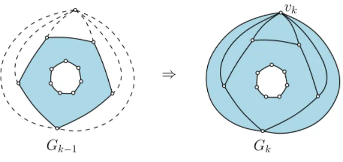
4.3 Canonical ordering
We first introduce a notion of canonical ordering for internally 3-connected cylindric maps. Before that, we need a bit of terminology. Given a pair (u, w) of outer active vertices, the outer path for (u, w) is the path, denoted γ(u, w), from u to w on the outer face contour, having the outer face on its left. The pair (u, w) is called consecutive if there is no active vertex in γ\{u, w}.
Definition 9. Let G be an internally 3-connected cylindric map with no active vertex for Cinn and with at least one active vertex for Cext. A canonical ordering for G is a growing sequence G0, G1, . . . , Gp of internally 3-connected cylindric maps such that:
• Initially, G0 = Cinn with all vertices active, at the end Gp = G. All along, the inner boundary-face of Gk is Binn. The outer boundary of Gk is denoted Ck.
• For k ∈ [0..p], the set of active vertices on Ck is the union of the set of those with at least one neighbour in G\Gk and the set of those that are on Cext and are active for G.7
• For k ∈ [1..p], Gk is obtained from Gk−1 either by:
– choosing a non-consecutive pair (u, w) of distinct active vertices on Ck−1 and connecting all active vertices on γ(u, w) to a newly added vertex in the outer face (see Fig.16(a));
– or choosing a consecutive pair (u, w) of distinct active vertices on Ck−1 and adding a path of at least two edges in the outer face connecting these two vertices (see Fig.16(b)).
• Additionally, for k ∈ [1..p], the vertices of Gk\Gk−1 must be active (for Gk).
Given a canonical ordering of G, the rank of a vertex v /∈ Cinn is the smallest k such that v∈ Gk. We prove the existence of such a canonical ordering by induction on the
7With these conditions it is easy to check that, since G has at least one active vertex for C
ext, then Gk
7 7 6 7 6 5 5 7 6 5 5 7 6 5 5 4 4 4 4 3 7 6 5 5 4 4 3 2 7 6 5 5 4 4 3 2 1 1 5 5 5 5 5 (a) (b) (c) (d) (e) (f) (g) (h) (i)
Figure 17: Shelling procedure to compute a canonical ordering of an internally 3-connected cylindric map (at each step the next deleted vertices are surrounded, the ranks of succes-sively shelled vertices are also indicated). The last drawing shows the cylindric map with the underlying forest and dual forest.
number of internal faces, which also yields a shelling procedure similar to the one described in the triangulated case. A first remark is that if G is not reduced to a cycle, then G must have an active vertex for Cext that is not on Cext\Cinn; indeed, if all the active vertices of G were on Cext∩ Cinn, it would easily yield a 2-separating curve not enclosing any active vertex, a contradiction. To describe the shelling procedure we need a bit of terminology. An internal face f is called separating if there is a separating 2-chord (always for Cext here) passing by f . A vertex on the outer face is called admissible if it is active, not on Cinn, and not incident to any separating face. Note that, by deleting an admissible vertex and declaring all its neighbours as active, one gets a cylindric map G0 such that G is obtained from G0 by applying the operation of Fig. 16(a). We now prove that either there is an admissible vertex or it is possible to get G from a cylindric map G0 with one less internal face by applying the operation of Fig. 16(b). For a given separating face f , the maximal separating 2-chord for f is the separating 2-chord c passing by f and such that the cycle enclosed by c is maximal (for the containment relation on the enclosed area). Consider the set E of maximal separating 2-chords associated to all separating internal faces of G. If E is not empty (i.e., there is at least one separating internal face), let c be a separating 2-chord
in E that is minimal (for the containment relation) and let f be the internal face to which c belongs. Two cases can occur. If the cycle enclosed by c contains no other internal face than f , then the subgraph Gc of G in the cycle enclosed by c (including the boundary of the cycle) is a path P that has at least two edges. Then by deleting the edges and internal vertices of P , and declaring as active the two extremities of P , we obtain a cylindric map G0 such that G is obtained from G0 by applying the operation of Fig. 16(b). Otherwise Gc contains at least one internal face f0. Among the separating 2-chords passing by f and whose enclosed cycle contains f0, let c0 be the minimal one (for the containment relation). Let P be the path on Cext inside c0, let u, w be the extremities of P . By minimality of c0, all vertices of P\{u, w} are not incident to f. In addition, at least one of these vertices has to be active (since G is internally 3-connected). Let v be such a vertex. By minimality of c, all internal faces (except for f ) in the cycle enclosed by c are non-separating, hence v is admissible since it is not incident to f . If E is empty, then there is no separating face. As we have seen, there is at least one active vertex on Cext\Cinn. Since there is no separating face, this vertex is admissible. To sum up, in all cases, it is possible to obtain G from a smaller cylindric map G0 by applying the operation of Fig. 16(a) or Fig. 16(b). It is also readily checked that the outer face of G0 is a simple cycle and that G0satisfies the conditions of Definition9. So we can continue inductively (starting from G0) until there just remains the cycle Cinn. This yields a shelling procedure to compute a canonical ordering satisfying Definition9. An example is shown in Fig. 17.
Let us now justify that the shelling procedure has linear time complexity. At each step, for each internal face f whose contour meets the current outer boundary Ck, we denote by V (f ) the number of outer vertices incident to f and by E(f ) the number of outer edges on the contour of f . Similarly as in Kant [18] for the planar case, we note that, at each step, an internal face is non-separating if and only if E(f )≤ 1 and V (f) = E(f) + 1; otherwise in the case where E(f )≥ 2 and V (f) = E(f)+1, then the face f can be shelled, corresponding to the reverse of the transition in Fig.16(b). At each step, for a current active outer vertex v, let N (v) be the number of separating faces incident to v. Note that v is admissible if and only if N (v) = 0 and v /∈ Cinn, in which case v can be shelled, corresponding to the reverse of the transition from Fig.16(a). By maintaining the quantities E(f ) and V (f ) for all internal faces touching the outer face, one can also maintain the quantities N (v) for all outer vertices (as well as their status: active or non-active). The shelling is done using two buffers S, S0: in S are stored the current admissible vertices, in S0 are stored the current faces f for which E(f )≥ 2 and V (f) = E(f)+1. At each step, at least one of the two buffers is non-empty (as we have proved above); so it suffices to shell the top-vertex from S or the top-face from S0, and then update the quantities E(f ), V (f ), N (v). Maintaining all these informations over the shelling procedure takes time O(|E|) (with |E| the number of edges of the cylindric map), which is also O(n) since|E| ≤ 3n. More details on implementing such a procedure in linear time are given by Kant [18] for the shelling procedure in the planar case.
Underlying forest and dual forest. Given an internally 3-connected cylindric map G with no chord at Cinn, and endowed with a canonical ordering π, we define the underlying forest F for π as the oriented subgraph of G where each active vertex v∈ Cexthas outdegree
0, and where each other vertex has exactly one outgoing edge, which is connected to the adjacent vertex u of v of largest rank in π. Since the edges are oriented in increasing labels, F is a spanning (oriented) forest; each component of the forest is rooted at each of the active vertices on Cext. The augmented map G (seen as a map on the sphere) is defined“
as the map obtained from G by adding a vertex w1 inside Binn, a vertex w2 inside Bext, and connecting all vertices around Binn to w1 and all active vertices around Bext to w2. We define F as F plus all edges (of“ G) incident to w“ 1 and all edges incident to w2. And
we define the dual forest F∗ for π as the graph formed by the vertices ofG“∗ (the dual of “
G) and by the edges of G“∗ that are dual to edges not in F . Each of the trees (connected“
components) of F∗ is rooted at a vertex “in front of” each edge of Binn, and the edges of the tree can be oriented toward this root-vertex (see Fig.17 bottom right). Similarly as in the triangulated case, for e∗ ∈ F∗, we call root-path of e∗ the path from e∗ to the root of the tree-component of F∗ to which e∗ belongs.
4.4 Periodic drawing algorithm for internally 3-connected cylindric maps with no active vertex for Cinn.
Given an internally 3-connected cylindric map G with no active vertex for Cinn, we first compute a canonical ordering of G, and then draw G in an incremental way, similarly as in the triangulated case. A first useful remark is that, at any step k, if we look at a path P of edges on Ck connecting two consecutive active vertices for Ck (i.e., P starts at an active vertex for Ck, ends at an active vertex for Ck, and all internal vertices of P are non-active), then P contains exactly one edge not in the underlying forest; this edge is called the bottom-edge of P . We start with a cylinder of width 2|Cinn| and height 0 (i.e., a circle of length 2|Cinn|) and draw the vertices of Cinn equally spaced on the circle: space 2 between two consecutive vertices (as in the triangulated case, it is possible to start with any configuration of points on a circle such that any two consecutive vertices are at even distance). Then the strategy for each k ≥ 1 is to compute the drawing of Gk out of the drawing of Gk−1. The difference with the triangulated case is that there are now two cases (those shown in Fig.16).
(a) Addition of one vertex and several internal faces. Consider the case of Fig.16(a); let v be the new added vertex, i.e., the unique vertex of Gk not in Gk−1. Let u1, . . . , us (with s≥ 2) be the neighbours of v on Ck−1, such that the path γ of Ck−1 from u1 to us has the outer face on its left. Let e1 be the first edge on γ and let e2 be the last edge on γ. There are two subcases. (1) If in the drawing of Gk−1 obtained so far, slope(e1) < 1 and slope(e2) >−1, then, as in the triangulated case, we place v at the intersection of the ray of slope 1 starting from u1 and the ray of slope −1 starting from us; and we draw all the edges from v to u1, . . . , us as segments. (2) If slope(e1) = 1 or slope(e2) = −1, let e` be the bottom-edge of the part of γ between u1 and u2 and let er be the bottom-edge of the part of γ between us−1 and us. Let P` (resp. Pr) be the root-path of e∗` (resp. e∗r) in F∗. Similarly as in the triangulated case (see Fig. 5), we stretch the cylinder by inserting a vertical strip of length 1 along P` and another one along Pr. After this, we insert (as in subcase (1)) the vertex v at the intersection of the ray of slope 1 starting from u1 and the
1 1 1 1 2 1 1 2 3 1 1 2 3 4 4 1 1 3 2 4 4 5 5 5 5 5 5 4 4 2 3 1 1 6 5 5 5 4 4 2 3 1 1 6 7
Figure 18: Complete execution of the algorithm computing an x-periodic drawing of an internally 3-connected cylindric map (no active vertex for Cinn). The steps follow the canonical ordering (in increasing order) computed in Fig. 17.
ray of slope −1 starting from us, and we connect v to all vertices u1, . . . , us by segments. The two rays from u1and us actually intersect at a grid point since the Manhattan distance between any two vertices on Ck−1 is even.
(b) Addition of one internal face. Consider the case of Fig.16(b), where we denote u, v1, . . . , vs, w (s≥ 1) the vertices of the new added chain, such that the path γ on Ck−1 from u to w has the outer face on its left. Let e1 be the first edge on γ and e2 the last edge on γ (note that e1 might be equal to e2). Let e be the bottom-edge of γ, and let P be the root-path of e∗ in F∗. There are two subcases. (1) If, in the drawing of Gk−1 obtained so far, slope(e1) < 1 and slope(e2) >−1, we insert a vertical strip of width 2s − 2 along P , increasing by 2s− 2 the x-span of each edge of Gk−1 dual to an edge in P . (2) If slope(e1) = 1 or slope(e2) = −1, we insert a vertical strip of width 2s along P , increasing by 2s the x-span of each edge of Gk−1 dual to an edge in P . Then we insert the vertices v1, . . . , vs into the drawing as follows. Let Ru be the ray of slope +1 from u and let Rw be the ray of slope −1 from w. Let q be the intersecting point of the two rays, denote by y(q) its y-coordinate; let S be the horizontal segment connecting Ru to Rw at ordinate y(q)− s + 1. Note that S has length 2s − 2. Then we insert v1, . . . , vsequally spaced (space 2 between two consecutive vertices) on S, with v1 at the left extremity and vs at the right extremity of S. And we draw the edges of the chain u, v1, . . . , vs, w as segments.
Fig. 18 shows the execution of the algorithm on the example of Fig. 17. The fact that the whole drawing of Gkremains crossing-free and weakly convex relies on the following inductive property, which is easily shown to be maintained at each step k from 1 to n:
Pl: In the upper boundary part γ between two consecutive active vertices —written (from left to right) as γ = P1, e, P2 with e the bottom-edge of γ— the edges of P1 have slope−1, e has slope in {−1, 0, 1}, and the edges of P2 have slope +1.
For each bottom-edge e on Ck, let Pe be the path in F∗ from e∗ to the root, let Ee be the set of edges dual to edges in Pe, and let δe be any nonnegative integer. Then the drawing remains planar when successively increasing by δe the x-span of all edges of Ee, for all bottom-edges e∈ Ck.
Remark 10. Clearly the resulting drawing has also the property that for each edge e∈ G, the absolute value of the slope of e is at most 1 if e /∈ F and is at least 1 if e ∈ F .
We now prove the bounds on the grid-size, where w is the width and h the height of the cylinder on which G is drawn. If |Cinn| = t then the initial cylinder is 2t × 0; and at each vertex insertion, the grid-width grows by 0 or 2. Hence w ≤ 2n. In addition, due to the slope conditions, the vertical span of every internal face f is not larger than the current width at the time when f is inserted in the drawing. Hence, if we denote by v the vertex of Cextthat is closest (at face-distance d) to Cinn, then the y-coordinate of v is at most d·(2n). And due to the slope conditions, the vertical span of Cext is at most w/2≤ n. Hence the grid-height is at most n(2d + 1). The linear-time complexity is shown next.
Linear-time complexity. The algorithm is completely similar to the one in the triangu-lated case. In a first pass one computes the y-coordinates of vertices and the x-span re of each edge e∈ G at the time t = k when e appears in Gk (as well one gets to know which extremity of e is the left-end vertex). Afterwards if e /∈ F and e /∈ Cext, the x-span of e might further increase due to the insertion of new vertices. Let se be the total further increase of the x-span undergone by e after its appearance. Let we ≥ 0 be the increase of the x-span undergone by e at the step k such that e∈ Ck−1and e /∈ Ckif such a step exists (otherwise we= 0). The quantity weis called the weight of e; the we’s can be computed in a first pass together with the quantities re. Let Te∗ be the subtree hanging from e∗ (including e∗) in the dual forest F∗, and let We be the sum of the weights of the dual of all edges in Te∗. Then, as in the triangulated case, se= We. Since the quantities se are easily computed in linear time from the quantities we, starting from the leaves and going up to the roots of F∗, this gives a linear time algorithm.
To sum up, we have proved Proposition8 for internally 3-connected cylindric maps with no active vertices for Cinn.
Remark 11. As in the triangulated case (Remark5), if we consider the initial-stretch vector R = (re)e∈Cinn and the final-stretch vector T = (te)e∈Cinn, then the vector S := T − R
is an invariant (it does not depend on R), because se = te − re only depends on the canonical ordering. Hence if a certain drawing yields final-stretch vector T , starting from initial-stretch vector R, then for any vector T0 of the form T + 2V —with V a vector of non-negative integers— one can redraw the graph to have final-stretch vector T0, by taking R0= R + 2V as initial-stretch vector instead of R.
Figure 19: Kant’s algorithm for internally 3-connected plane graphs is recovered from our algorithm by adding a vertex of degree 2 to complete the inner boundary.
Remark 12. Our algorithm extends Kant’s algorithm [18], which works for internally 3-connected planar maps, i.e., planar maps with a simple outer face contour and where all 2-separating curves have to pass by the outer face. Indeed, if we are given an internally 3-connected plane graph G (with an outer root-edge) we can turn it into a cylindric internally 3-connected map ˜G by adding a vertex of degree 2 connected to the two extremities of the root-edge; we also declare as active all outer vertices of ˜G that are not one of the three vertices of the inner boundary. Then, Kant’s drawing of G is recovered from the periodic drawing of ˜G upon deleting the added vertex of degree 2, see Fig.19.
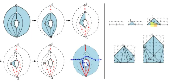
4.5 Allowing for non-contractible 2-separating curves (no active vertex on Cinn). The method based on a canonical ordering and incremental drawing algorithm is easily ex-tended to essentially internally 3-connected maps with no 1-separating curve. Additionally we require here that at least two outer vertices are active (the case of one outer vertex active will be handled in the next section). Let G be such a cylindric map. The definition of canonical ordering for G is exactly the same as for internally 3-connected cylindric maps, adding the possibilities that Gk is obtained from Gk−1 as shown in Fig.20.
Such a canonical ordering can be computed by a shelling procedure that extends the one of Section 4.3. Call a 2-separating curve internal if it passes by two internal faces and does not pass by two outer vertices. In terms of the associated corner-map S such a 2-separating curve corresponds to a separating 4-cycle where the two incident white vertices (vertices of the cylindric map) are not both on Cext. This time, a vertex on the outer boundary and not on the inner boundary is called admissible if it is not incident to a separating face nor incident to an internal 2-separating curve. By the same arguments as in Section4.3, one can show that if there is a separating face, then either there is an admissible vertex (which can be shelled) or there is an internal face sharing a path of r≥ 2 edges with
⇒
Gk−1 Gk
⇒
Gk−1 Gk
Figure 20: When non-contractible 2-separating curves are allowed (and there are at least two active vertices for Cext), the additional cases shown here might occur for the transition from Gk−1 to Gk.
the outer boundary (which can be shelled). If there is no separating face but there is at least one internal 2-separating curve, one can check that, if two vertices of Cext are incident to an internal 2-separating curve, then one must be in the situation in the right-part of Fig. 20. Otherwise at most one vertex of Cext is incident to a 2-separating curve, and since there are at least two outer vertices active, at least one of them is admissible. Finally, in case there is no separating face nor 2-separating curve, then any active outer vertex is admissible and can be shelled. One can continue shelling iteratively until there just remains Cinn (since there is no 1-separating curve, it is easy to see that the property of having at least two active outer vertices is automatically maintained). A linear time algorithm is also readily obtained by maintaining, for each outer vertex, how many separating faces and how many internal 2-separating curves it is incident to. Note that such a canonical ordering also induces an underlying forest F and a dual forest F∗. Finally, the incremental drawing algorithm (and linear complexity using the dual forest) works in the same way as for internally 3-connected cylindric maps. An example is shown in Fig.21, where the situation corresponding to the right-part of Figure20 is shown in the last step of the drawing.
The grid bounds are also the same as for internally 3-connected cylindric maps (the arguments to obtain the bounds in the simple case did not use the fact that there are no 2-separating curves). So this gives Proposition 8 for essentially internally 3-connected cylindric maps with no 1-separating curve and with at least two outer vertices active. Finally, Remark11 still holds here (the arguments are the same).
4.6 Allowing for 1-separating curves (no active vertex for Cinn).
We finally explain how to deal with 1-separating curves. Similarly as in the triangulated case, we do not extend the notion of canonical ordering but simply decompose (at 1-separating curves turned into loops) such a cylindric map into a “tower” of components separated by loops. Let G be an essentially internally 3-connected cylindric map with n vertices. Note that if G has a loop e, then there is a 1-separating curve “just inside” e (if e is not Cinn) and there is a 1-separating curve “just outside” e (if e is not Cext).