A Continuous Silent Speech Recognition System for
AlterEgo, a Silent Speech Interface
by
Eric J. Wadkins
B.S., Massachusetts Institute of Technology (2018)
Submitted to the
Department of Electrical Engineering and Computer Science
in partial fulfillment of the requirements for the degree of
Master of Engineering in Electrical Engineering and Computer Science
at the
MASSACHUSETTS INSTITUTE OF TECHNOLOGY
June 2019
c
○ Massachusetts Institute of Technology 2019. All rights reserved.
Author . . . .
Department of Electrical Engineering and Computer Science
May 24, 2019
Certified by . . . .
Pattie Maes
Professor, Media Arts and Sciences
Thesis Supervisor
Accepted by . . . .
Katrina LaCurts
Chair, Master of Engineering Thesis Committee
A Continuous Silent Speech Recognition System for AlterEgo,
a Silent Speech Interface
by
Eric J. Wadkins
Submitted to the Department of Electrical Engineering and Computer Science on May 24, 2019, in partial fulfillment of the
requirements for the degree of
Master of Engineering in Electrical Engineering and Computer Science
Abstract
In this thesis, I present my work on a continuous silent speech recognition system for AlterEgo, a silent speech interface. By transcribing residual neurological signals sent from the brain to speech articulators during internal articulation, the system allows one to communicate without the need to speak or perform any visible movements or gestures. It is capable of transcribing continuous silent speech at a rate of over 100 words per minute. The system therefore provides a natural alternative to normal speech at a rate not far below that of conversational speech. This alternative method of communication enables those who cannot speak, such as people with speech or neurological disorders, as well as those in environments not suited for normal speech, to communicate more easily and quickly. In the same capacity, it can serve as a dis-creet, digital interface that augments the user with information and services without the use of an external device.
I discuss herein the data processing and sequence prediction techniques used, describe the collected datasets, and evaluate various models for achieving such a con-tinuous system, the most promising among them being a deep convolutional neural network (CNN) with connectionist temporal classification (CTC). I also share the results of various feature selection and visualization techniques, an experiment to quantify electrode contribution, and the use of a language model to boost transcrip-tion accuracy by leveraging the context provided by transcribing an entire sentence at once.
Thesis Supervisor: Pattie Maes
Acknowledgments
I am privileged to have had the opportunity to think, work, and learn surrounded by so many incredible people at MIT. They will continue to serve as an inspiration to me.
I would like to thank my advisor, Prof. Pattie Maes, and project lead, Arnav Kapur, as well as so many others in the Media Lab’s Fluid Interfaces Group, for providing guidance and mentorship throughout the course of my Master’s program.
Finally, I would like to thank my family and friends for their continued support this past year and throughout my entire time at MIT. It would not have been possible without them.
Contents
1 Introduction 17
1.1 Motivation . . . 19
1.2 Background and Related Work . . . 20
1.2.1 Automatic Speech Recognition . . . 20
1.2.2 Silent Speech . . . 21
1.2.3 Sequence-to-Sequence Models . . . 24
2 Approaches 27 2.1 Signal Capture and Processing . . . 27
2.1.1 Signal Capture . . . 27
2.1.2 Correcting for DC Offset and Baseline Drift . . . 29
2.1.3 Noise Removal Techniques . . . 30
2.2 Feature Selection and Visualization . . . 33
2.2.1 Wavelet Convolutions . . . 33
2.2.2 K-Means Clustering . . . 35
2.2.3 Autoencoder and PCA of the Latent Space . . . 36
2.3 Sequence Prediction . . . 39
2.3.1 Dual Word and Activation Classifier . . . 40
2.3.2 Connectionist Temporal Classification (CTC) . . . 41
2.3.3 LSTM with CTC . . . 44
2.3.4 CNN with CTC . . . 46
3 Datasets and Testing Procedures 51
3.1 Dataset Limitations . . . 51
3.1.1 Lack of Applicable Datasets . . . 51
3.1.2 User and Session Dependence . . . 52
3.2 Recorded Datasets . . . 53
3.2.1 Digit Sequence Datasets . . . 53
3.2.2 10-Word Vocabulary, 20-Sentence Dataset . . . 53
3.2.3 20-Word Vocabulary, 200-Sentence Dataset . . . 55
3.2.4 Subvocal Phonemes and Syllables . . . 57
3.3 Testing Procedures . . . 57
4 Evaluation 59 4.1 Metrics . . . 59
4.1.1 Average Normalized Edit Distance . . . 59
4.1.2 Rate of Speech and Information Transfer Rate . . . 60
4.2 Model Comparison . . . 61
4.2.1 Digit Sequence Datasets . . . 61
4.2.2 10-Word Vocabulary, 20-Sentence Dataset . . . 63
4.2.3 20-Word Vocabulary, 200-Sentence Dataset . . . 64
4.3 Language Model . . . 65
4.4 Electrode Contribution . . . 68
5 Conclusion 71 5.1 Summary of Results . . . 71
5.2 Conclusion and Discussion . . . 73
5.3 Future Work . . . 74
A Tables 77
B Figures 79
List of Figures
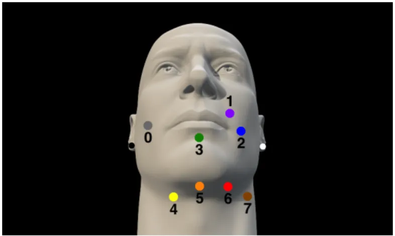
2-1 A typical arrangement of 8 signal electrodes (colors and gray, on face and neck) and reference and bias electrodes (white and black, inter-changeable on earlobes). . . 28 2-2 The unprocessed signal of a sequence of three words ("tired", "hot",
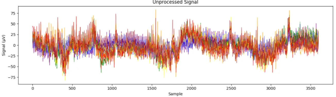
"i"). The 8 data channels are colored according to the electrode place-ment shown in Figure 2-1. . . 29 2-3 The DC offset (left) and baseline drift (right) of an unprocessed signal
over about 3 minutes. The signals in the right plot are normalized by their initial value to show the baseline drift, but in reality are the same as in the left plot. . . 29 2-4 A Butterworth highpass filter is used to remove frequencies less than
0.5 Hz. The uncorrected signal (top) baseline drifts significantly over a period of only about 3.5 seconds, whereas the highpassed signal (bot-tom) does not. . . 30 2-5 Several Butterworth notch filters, with bands at multiples of 60 Hz,
are used to remove the power line hum. The notch-filtered signal and its frequency domain (bottom) show almost no noise at multiples of 60 Hz, unlike the signal with power line interference (top). . . 31 2-6 A Ricker wavelet (left) is convolved with a signal with heartbeat
ar-tifacts (top). The convolution (middle) is then subtracted from the signal, resulting in approximate removal of heartbeat artifacts without significantly distorting the original signal (bottom). . . 32
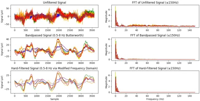
2-7 A Butterworth bandpass filter is applied to a signal (top) to remove most noise outside the frequency band 0.5-8 Hz, resulting in clearly visible low-frequency features (middle). Alternatively, modifying the frequency domain removes completely all frequencies outside of this band (bottom). . . 33
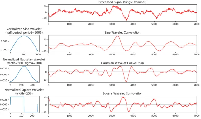
2-8 Examples of normalized sine, Gaussian, and square wavelets, all cen-tered around zero, and the corresponding convolutions on an example signal. . . 34
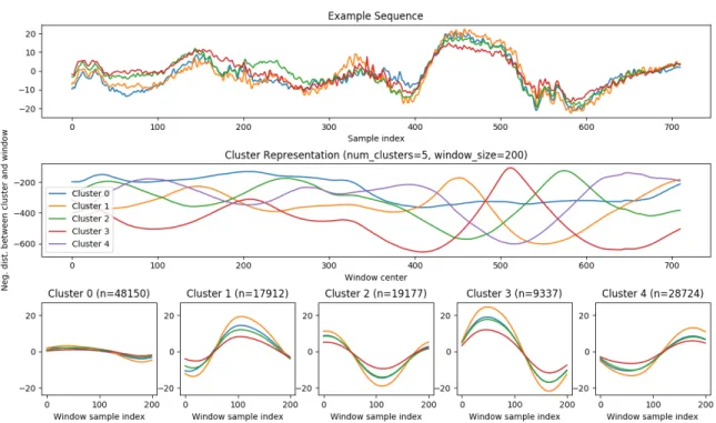
2-9 An example sequence (top), the clusters chosen from a large dataset of similar sequences (bottom), and the cluster representation of the example sequence (middle). . . 35
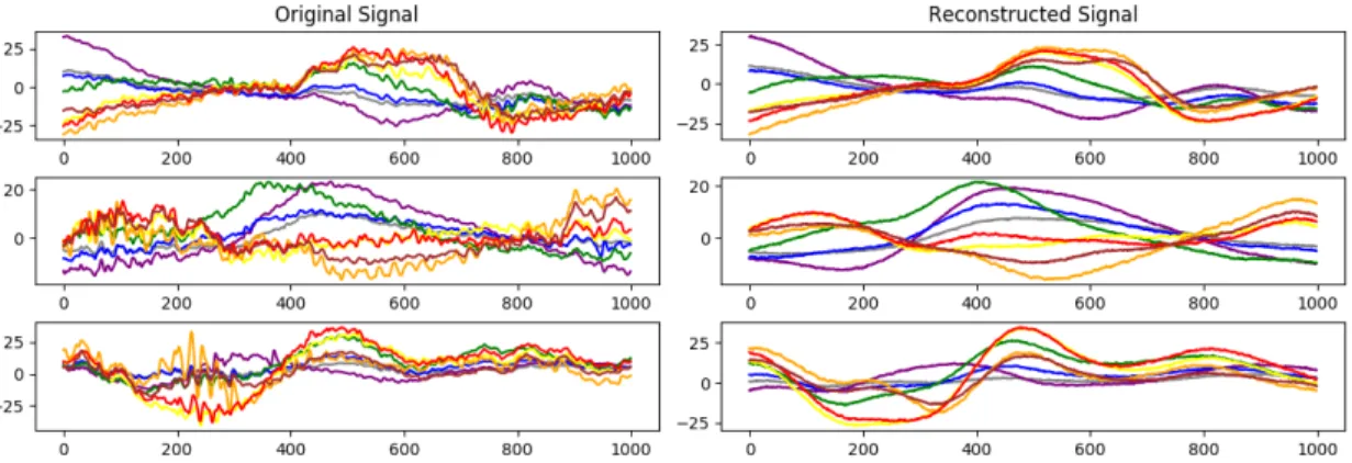
2-10 Example output from an autoencoder with a window size of 1000 sam-ples. One can see that signals reconstructed from the autoencoder’s condensed representation are devoid of smaller, high-frequency fea-tures, which the autoencoder cannot afford to encode in only 32 units of information. It also removes less common features, like periods of extreme noise that occur very rarely. . . 37
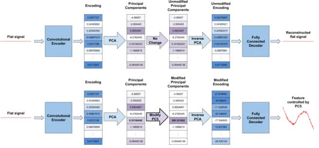
2-11 The changes to the reconstructed signal upon modifying one of the principal components reveals what features have been learned by the autoencoder that are controlled by that component. The process with-out any changes to the principal components is shown on top, and the results upon modifying PC5 are shown on bottom. . . 38
2-12 The effect of each principal component on the reconstructed signal, us-ing an autoencoder with latent size 32. Visualizus-ing the effects is done by manually modifying the principal components in the transformed encoding space and seeing the change in the reconstructed signal. Also shown is the explained variance, or eigenvalue, of each of the princi-pal components, which gives a measure of how prevalent the features controlled by each component are. One can see that the first 6 or 7 principal components control very distinct features, whereas the higher principal components seem to have features in common, or show no sig-nificant features at all. This is reflective of the features actually seen in the dataset. . . 39
2-13 A comparison of the single-word prediction and sentence prediction pipelines, showing the minimal difference in structure and function of the two architectures. . . 42
2-14 The use of a bidirectional LSTM model for temporal feature extraction followed by sequence prediction using CTC. This figure shows a two-layer bidirectional LSTM with one fully connected two-layer, although it is common to use more layers. . . 45
2-15 The details of the LSTM architecture used in evaluation of an LSTM with connectionist temporal classification (CTC). . . 45
2-16 The use of a CNN model for window feature extraction followed by sequence prediction using CTC. This figure shows a three-layer CNN with one fully connected layer and an output softmax layer, although it is common to use more layers. . . 46
2-17 The details of the CNN architecture used in evaluation of a CNN with connectionist temporal classification (CTC). . . 47
3-1 In this example, if in all training sentences every occurrence of the word "i" is followed by "need" and every occurrence of the word "need" is preceded by "i", then incorrect alignments such as those shown above may be learned. . . 55 3-2 The distribution of rates of speech in the 20-word vocabulary,
200-sentence dataset, reported in words per minute (WPM). 1000 samples of sentences were collected in total. The average is 102.4 WPM, with 62% of samples having a rate of speech of at least 100 WPM. . . 56 4-1 The training and validation confusion matrices for the task of
classify-ing digits 0 through 9. . . 63 4-2 Comparison of error rates of the CNN with CTC model with and
with-out a language model. . . 66 4-3 Comparison of error distributions of the CNN with CTC model with
and without a language model when near fully trained. Note that the top-10 error rates with and without a language model are the same. The differences between these top-k error rates give a measure of where in the k most probable predictions the highest-accuracy predictions re-side. For example, a large difference between the top-k and top-(k+1) error rates indicates that some (k+1)th most probable predictions are higher in accuracy than the corresponding kth most probable predic-tions. This, in turn, signals that the accuracy of the system could be improved if the probabilities of the predictions could be better corre-lated with their accuracies. . . 67 4-4 Left: The arrangement of 8 signal electrodes (colors and gray, on face
and neck), with reference and bias electrodes also shown (white and black, on earlobes). Right: The relative electrode contributions, rep-resented by the sizes of the electrode markers. . . 69 B-1 Examples of signals recorded for each of the 20 sentences in the 10-word
B-2 Examples recordings for 20 of the 200 sentences in the 20-word vocab dataset. The signals shown here have visibly fewer features than the signals of the 10-word vocab dataset (shown in Figure B-1). This is due to the much higher rate of speech of this dataset (over 100 WPM). 81
List of Tables
3.1 The 10 vocabulary words and the 20 sentences constructed from the 10 word vocabulary such that no two sentences share a bigram. The sentences are nonsensical, but this is acceptable (even somewhat desir-able) for the task of learning the alignment between individual words. Example recordings of these sentences can be seen in Figure B-1 in Appendix B. . . 54
3.2 The 20 vocabulary words chosen to make up the 200 sentences. The 200 sentences we generated from this vocabulary can be found in Appendix A. . . 56
4.1 Example test output of the 0-1-2 permutation sequence labeling task. Incorrect predictions and the corresponding target sequences are bolded. 62
4.2 Example test output of the 10-word vocabulary sequence labeling task. Incorrect predictions and the corresponding target sequences are col-ored red. . . 64
4.3 Example test output of the 20-word vocabulary sequence labeling task. Incorrect predictions and the corresponding target sequences are col-ored red. . . 65
4.4 The top 10 predictions with and without a language model, in order of decreasing probability, for an example sequence. The predictions are colored green, yellow, or red, depending on if they have an edit distance from the target sequence of 0, 1, or 2, respectively. This example is an instance of the most probable prediction being correct only with the use of a language model. Note: there are many repetitions, since the CTC decoder outputs each prediction independent of all others. . . . 68 4.5 The calculated electrode contributions, shown visually in Figure 4-4. . 70 5.1 The final accuracy/error rates achieved by each approach, evaluated
against each of the collected datasets. We report the single-label clas-sification accuracy of a simple CNN on each of the datasets (as a single-label baseline), as well as the sequence prediction error rates (i.e. av-erage normalized edit distances) for all of the sequence-to-sequence approaches. While the LSTM with CTC approach was tested on all three of the datasets presented here, drastically longer training times and the lack of large datasets prevented us from fully training and optimizing the LSTM. Therefore, we only report the error rate of the unoptimized LSTM approach for one dataset. . . 72 A.1 The 200 sentences generated from the 20 word vocabulary. While some
sentences shown are grammatical (eg. "what am i doing", "i am hun-gry"), most of the sentences are nonsensical, to aid in training the model to learn the alignment between words. Still, there are many phrases contained in the nonsensical sentences that are quite common (eg. "how are youwant i") that may actually be used in practice. . . . 78
Chapter 1
Introduction
As humans, we have an incredible ability to understand information presented to us. We are fortunate for this, as information plays a fundamental role in our lives. Our decision making process is driven by access to information. And communication, the means through which we share knowledge and form relationships with others, is, at its simplest, the transfer of information. For this reason, access to information (or lack thereof) is a limiting factor in what we can achieve, and can potentially interfere with our ability to problem solve and communicate. Internet-connected computing devices, on the other hand, have unmatched access to information, as well as the computing power to solve many problems humans do not have the capacity to solve. Still, machines cannot yet replace humans in performing many tasks. Therefore, a natural solution arises – the coupling of human and machine, using the strengths of both to more effectively achieve the user’s goals.
AlterEgo is a silent speech interface that aims to augment a human user with the information and computing power available to a computing device, while also providing an alternative means of communication. It is a wearable device, as detailed by Kapur et al. [1] [2], that allows a user to communicate without any speaking or visible movement. Unlike devices that listen for speech, AlterEgo reads residual neurological signals produced during internal articulation or "silent speech" – often described as one’s inner voice, which generally manifests as the slight activation of the internal speech system. The system then uses machine learning to transcribe
those signals into text. The resulting system is one that can be used similarly to a voice-controlled virtual assistant, but without the need to actually speak or perform any visible movements or gestures. When paired with a discreet feedback device, such as bone conduction headphones, it gives the experience of having an AI or virtual assistant in one’s head.
In this thesis, I present my work on a continuous silent speech recognition system for AlterEgo as part of the research of the Fluid Interfaces Group at the MIT Media Lab. By transcribing residual neurological signals sent from the brain to speech artic-ulators during internal articulation, the system allows one to communicate without the need to speak or perform any visible movements or gestures. It is capable of transcribing continuous silent speech at a rate of over 100 words per minute. The system therefore provides a natural alternative to normal speech at a rate not far below that of conversational speech. This alternative method of communication en-ables those who cannot speak, such as people with speech or neurological disorders, as well as those in environments not suited for normal speech, to communicate more easily and quickly. In the same capacity, it can serve as a discreet, digital interface that augments the user with information and services without the use of an external device.
I discuss herein the data processing and sequence prediction techniques used, describe the collected datasets, and evaluate various models for achieving such a con-tinuous system, the most promising among them being a deep convolutional neural network (CNN) with connectionist temporal classification (CTC). I also share the results of various feature selection and visualization techniques, an experiment to quantify electrode contribution, and the use of a language model to boost transcrip-tion accuracy by leveraging the context provided by transcribing an entire sentence at once.
1.1
Motivation
There are various scenarios in which normal speech is not a viable method of commu-nication. A system capable of transcribing internally articulated words provides an alternative method of communication, whether it be with another person or with a computing device/virtual assistant. In the latter case, the system can serve as a dis-creet, digital interface that augments the user with information and services without the use of an external device and the disruption from one’s environment that often comes with it.
First, the user may not wish to speak out loud for a few reasons. One such reason is that the topic may be personal or not desirable to mention in public. The user may also be in a public setting where others don’t want to be disturbed, such as on an airplane or in a library. In situations like these, most people would generally opt for physically interacting with a device, such as their phone, in order to communicate. However, the need to physically interact with a device that could otherwise be used tangentially may serve as a distraction or an inconvenience when trying to complete a task. Second, the setting may not be conducive to a normal conversation with another person or a device. For example, one may be near a large crowd or in a factory, where the surrounding noise makes normal speech difficult to discern. In this case, conversation or use of a voice-controlled virtual assistant is not just undesirable, but infeasible.
Finally, and most importantly, many people have difficulty speaking or are un-able to speak entirely (conditions known collectively as dysarthria) due to a variety of speech or neurological disorders. The National Institute on Deafness and Other Com-munication Disorders [3] states that approximately 7.5 million people in the United States alone (over 2%, by Feb. 2019 UN estimates) have trouble using their voices to communicate. All of the conditions associated with dysarthria affect one’s ability to speak, but many do not affect one’s ability to internally articulate, the result of residual signals from neuromuscular pathways that remain functional. In fact, several user studies on the use of AlterEgo by ALS and MS patients showed that all
partici-pating patients, with varying stages of their respective disorder, were able to produce signals to the same extent as someone without any speech or neurological disorder. Furthermore, in successful user trials, several patients with ALS and MS were able to use our system to accurately transcribe a small vocabulary of silent speech into text, which was then spoken aloud using text-to-speech software. Current systems that allow affected patients to speak, known as speech generating devices, are slow to use as they rely on an unnatural means of input, such as a headmouse or eye gaze. Many are also tiring to use and prevent the user from making eye contact with others while communicating. Therefore, a system that can accurately transcribe sentences from internal articulation, a fairly natural means of input, and do so in real-time, could potentially help millions of people communicate more easily.
1.2
Background and Related Work
Much work has been published on automatic speech recognition systems, and large datasets have enabled rapid advancement in the field. Far less work has been pub-lished with a focus on automatic recognition of silent speech, and doing so continu-ously without any visible movement.
1.2.1
Automatic Speech Recognition
Automatic speech recognition (ASR) systems are systems capable of transcribing speech into written language. The capabilities of ASR systems vary greatly, so one must be more specific when discussing these systems. In their review of speech recog-nition systems, Saksamudre et al. [4] introduce a classification scheme based on a system’s robustness and level of understanding of natural speech. The scheme clas-sifies systems into the following levels, listed by level of understanding from most-limited to most-inclusive: isolated-words, connected-words, continuous speech, and spontaneous speech. The two levels relevant to this work are connected-words and continuous speech systems. Connected-words systems recognize primarily individual words, although they may recognize several words in succession with sufficient pauses
between them. Users of these systems must be aware of the constraint placed on them – a pause or delimiter signal of some sort is necessary for accurate transcription of more than one word. This limits their ability to communicate naturally and at a high rate of speech. These models also only take as input a single word at a time, which results in each word being predicted independent of all others. The original AlterEgo system, as described by Kapur et al. [1] [2], was a connected-words system, and therefore was subject to all of the aforementioned problems. Continuous speech systems, on the other hand, eliminate the need for clear divisions between words and are able to transcribe entire sentences or phrases at a time. The system presented in this thesis is categorized as a continuous speech system for this reason. Another benefit of this type of system is that the input is an entire sentence or phrase, so the context provided by surrounding words can be utilized in the prediction process to improve prediction accuracy.
Continuous speech recognition systems for audible speech are already ubiquitous in today’s world, and the technology is a major selling point for countless new de-vices. Speech is a particularly rich input modality, and the technology required to capture audio signals is no barrier to the development of these systems – even simple microphones generally record at incredibly high sampling rates with very little sys-temic noise. There are also many large datasets that can be used to train a speech recognition system on regular speech. Unfortunately, none of the same can be said for the modality of silent speech, making the development of reliable continuous silent speech recognition systems an active area of research.
1.2.2
Silent Speech
The term "silent speech", as used in this thesis, refers specifically to internal artic-ulation, which is the deliberate but subtle neurological activation of internal speech articulators that is often observed while reading very intently. Importantly, this action does not result in any sound or visible movement. In other papers, the term "silent speech", as well as the more loosely-defined terms "subvocalization" and "subvocal speech", are often used to describe actions that result in some visible movement or
audible speech. Regardless of the level of movement or sound involved, all types of subvocalization are a natural means of input as derivatives of natural speech. With silent speech, rather than performing a gesture or coded interaction to indicate a specific intent, one only needs to silently speak their intent, as if talking to oneself internally. This is also arguably a more natural means of input than using a physical device like a keyboard or mouse, as with these devices we must learn how to efficiently express our ideas, unlike with natural speech. Therefore, silent speech shares all the benefits of communicating with regular speech, without the need for any overt action by the user.
Research into subvocalization started as early as 1970 when Eriksen et al. [5] and, later in 1973, Klapp et al. [6], explored the concept of "implicit speech" in reading. It was suggested that subvocalization may play a role in subjects’ understanding of previously unseen words, as they would often pause and subvocalize new words prior to reading them out loud. For this reason, subvocalization was thought to be a precursor of spoken language, or another representation of the spoken language itself. This, coupled with drastic improvements in speech recognition systems over the years, led researchers to consider the possibility of transcribing subvocal speech into text.
The NASA Ames Research Center began research into subvocal speech recogni-tion systems in 2003. In one paper, Jorgensen et al. [7] describe training a neural network model to recognize 6 to 10 subvocal words, including digits zero through nine. Their system used sub-audible (or sotto voce) speech and relied on electromyo-graphic (EMG) signals from visible muscle movement – a clear distinction from our system. Using 100 training samples of each word, they achieved an accuracy of 92% on recorded test samples. Their conclusion upon experimenting with larger vocabularies is that a 20-word recognition task seems feasible, but recognition of a significantly larger vocabulary is not. As such, they suggest that the system be used with a small vocabulary specialized to the task at hand. They also mention that the system still suffers from being specific to a single user and sensitive to noise, electrode locations, and physiological changes in the user. These issues have been found to affect the AlterEgo system as well.
Several other research groups have experimented with subvocal speech recognition systems. There has been significant exploration in using invasive systems with direct brain implants to recover signals generated during subvocal speech. Brumberg et al. [8] report that the use of intracortical microelectrode arrays shows promising results in early-stage trials with the goal of providing a speech prosthetic. Similarly, in a recent Nature article, Anumanchipalli et al. [9] discuss their method of synthesizing intelligi-ble speech from high-density electrocorticography (ECoG) signals. Using ECoG data collected from patients while audibly speaking sentences at a normal conversational rate, they are able to decode the signals into an intermediate audio spectrogram, and then into sythesized speech. Sentence-level intelligibility tests, which asked subjects to listen to and transcribe the synthesized speech, reported word error rates of 31% for a 25-word vocabulary, and 53% with a 50-word vocabulary. These results were for fully-audible speech, while they report that results for mimed speech (still with significant visible movement) were significantly worse.
There has also been significant exploration of non-invasive systems, with the hope of scaling beyond clinical use. Wand et al. [10] use a non-invasive system to transcribe EMG signals from subvocal speech into text, achieving a fairly low word error rate on a large vocabulary, but with clearly visible movements of the mouth. This work is continued by Jou et al. [11], who evaluate a continuous subvocal speech recognition system, but still with significant movements and a high word error rate.
All known studies, including those mentioned here, deviate from the goals of Al-terEgo in a significant way. The vast majority focus only on transcribing individual words with a connected-words level system or continuous speech with a low tran-scription rate. As previously mentioned, the drawback of this, other than taking significantly longer to communicate the same amount of information, is that the sys-tem requires a significant pause between words and therefore feels much less natural to use. The primary goal of our system, however, is to transcribe continuous silent speech with a relatively high transcription rate. The few studies that do use continu-ous recognition systems do not focus on transcribing internal articulation specifically. Instead, their focus is on transcribing subvocal speech with significant movement of
mouth or facial muscles, or with significant sound produced. While this is acceptable in many situations, our use cases require little to no visible movement or sound, es-pecially if our system is to aid patients who are unable to exert this level of muscular control.
1.2.3
Sequence-to-Sequence Models
Continuous speech recognition systems make use of sequence-to-sequence models, also known as sequence prediction or sequence generation models. These models produce a variable-length sequence as output, as opposed to the fixed length output produced by classification models. Continuous speech recognition requires the use of these mod-els because the input to the system is a signal representing an entire sentence, and the output is a variable-length sequence of words which form the full transcribed sen-tence. Other examples of tasks that require sequence-to-sequence models are machine translation, handwriting recognition, image captioning, and speech generation.
The learning process for sequence-to-sequence models differs significantly from that of classification models. Using continuous speech recognition as an example, not only must the model learn to classify portions of a signal as the correct word, it must also learn how many words are present in the input signal and which portions of the input signal correspond to each word in the output sequence. This surjective function of input to output that must be learned by the model is known as the alignment. For some applications, the ordering of the input and output segments may not be the same, as is the case with machine translation due to grammatical differences between languages. Fortunately, this is not the case for speech/silent speech recognition systems, though, because the words in a sentence are always said in the same order that they are written. This simple fact provides greater flexibility in choosing a sequence-to-sequence modeling approach, which will be discussed in more detail in Section 2.3.
The traditional approach to label sequence prediction, before heavy use of the now-common recurrent neural network (RNN) encoder-decoder models, was to use a hybrid neural network and hidden Markov model (HMM) model. The neural network would
be used for classification at each timestep of the input sequence, and the HMM would decode these predictions into the output label sequence, as discussed by Juang et al. [12] in the context of speech recognition with HMMs. However, the need to train both the classifier and decoder separately is undesirable. Currently, the most commonly used approach for sequence prediction is the use of RNN encoder-decoder models. As explained by Lu et al. [13], the approach uses an encoder RNN model to transform the input sequence into a fixed-length vector representation, and a decoder RNN model to transform the fixed-length vector, which theoretically contains information on the entire input sequence, into an output sequence of labels. The loss is calculated from the output of the decoder model, but because the decoder takes as input the output of the encoder model, the two are trained simultaneously during loss optimization. There are, however, a few downsides to using this approach. For long-term dependencies to be reliably modeled, one must use a long short-term memory (LSTM) or gated recurrent unit (GRU) model, both of which are slow to train. A simple RNN with a less complicated activation function takes far less time to train than an LSTM or GRU, but due to the issue of exploding/vanishing gradients [14], cannot manage long-term dependencies. Also, RNNs in general are prone to overfitting, resulting in poor generalization. The approach primarily used in this work, known as connectionist temporal classification, is capable of overcoming both of these obstacles because of its simplicity and ability to be used with either an RNN or CNN (see Sections 2.3.3 and 2.3.4).
Chapter 2
Approaches
This chapter will describe the signals of interest and how they are captured, the signal processing techniques used to separate meaningful features from noise, several methods of feature selection and visualization, and the machine learning approaches used to transcribe these signals into a sequence of words. Additionally, we detail the integration of a language model for increased sequence prediction accuracy.
2.1
Signal Capture and Processing
2.1.1
Signal Capture
In creating a subvocal speech recognition system, the signals of interest are the in-dividual neurological activations of internal speech articulators. As a non-invasive device, there is no way for AlterEgo to directly record these signals. Instead, they must be collected externally, far from the actual source. The best method for doing this is with electrodes that can pick up on subtle disruptions in the electric field surrounding speech articulators. With these electrodes placed on the face and neck regions, as in Figure 2-1, an aggregation of the desired neuromuscular signals is ap-parent during internal articulation. The device uses 8 signal electrodes and reference and bias electrodes, measuring the potential difference between each signal electrode and the reference electrode (with the bias electrode used for on-device data
process-Figure 2-1: A typical arrangement of 8 signal electrodes (colors and gray, on face and neck) and reference and bias electrodes (white and black, interchangeable on earlobes).
ing). Figure 2-1 shows a typical arrangement of the electrodes. This arrangement, or at times a subset of the electrodes, is used in all experiments detailed in this paper. Many subsets of these 8 signal electrodes have been used without a noticeable drop in accuracy, as some of the electrodes capture similar signals due to proximity to the same muscles. For example, all electrodes placed on the neck (electrodes 4-7 in Figure 2-1), capture highly correlated signals, and therefore the system generally performs the same with just one or two of them.
This method of using surface electrodes to capture signals from internal articu-lation also captures a large amount of noise introduced by the body, as would be expected when collecting distant physiological signals. The data collection device also introduces a secondary source of noise, as well as a slight baseline drift in the signals over time. This noise proves troublesome because the signals collected via this method, as shown in Figure 2-2, are already comparatively weak (generally in the range of single digit to low double digit microvolts), resulting in data with a low peak signal-to-noise ratio. Therefore, some signal processing is required to extract the features of interest before a model can learn from the data.
Figure 2-2: The unprocessed signal of a sequence of three words ("tired", "hot", "i"). The 8 data channels are colored according to the electrode placement shown in Figure 2-1.
Figure 2-3: The DC offset (left) and baseline drift (right) of an unprocessed signal over about 3 minutes. The signals in the right plot are normalized by their initial value to show the baseline drift, but in reality are the same as in the left plot.
2.1.2
Correcting for DC Offset and Baseline Drift
The variation in electrode placement relative to the reference electrode creates a large DC offset, which manifests as a seemingly arbitrary offset in each data channel. Ad-ditionally, the device used to record potential differences between signal and reference electrodes introduces a very low frequency source of noise. While this noise is low enough in frequency that it affects only the baseline, or long-term mean amplitude of a signal, this drift is rapid enough that the baseline can drift by up to a few hundred microvolts (an order of magnitude larger than the amplitude of the signal of interest) in less than a minute. These two effects are clear in signals collected over a long period of time, as shown in Figure 2-3. They are also apparent on shorter time scales, albeit much more subtly. The rate and direction of baseline drift is unpredictable and the
Figure 2-4: A Butterworth highpass filter is used to remove frequencies less than 0.5 Hz. The uncorrected signal (top) baseline drifts significantly over a period of only about 3.5 seconds, whereas the highpassed signal (bottom) does not.
baseline of each channel changes independently of the others. This negatively affects a model’s ability to recognize features within a signal, as the relative amplitudes of channels change in a way that is difficult for a model to learn.
To remove these artifacts, the signals are normalized by their initial values and frequencies lower than 0.5 Hz are highpassed out using a 1st-order Butterworth filter. Initial value normalization prior to the filtering is necessary to avoid severe artifacts upon applying the Butterworth filter. Afterwards, the signals are normalized such that the mean amplitude is zero, in order to center the signals. Figure 2-4 shows the drift correction for a single recording of about 3.5 seconds in length. With the correction, one can see the correlation of channel amplitudes across channels, which is less obvious without the removal of the baseline drift.
2.1.3
Noise Removal Techniques
There are three sources of noise present in our data, after the DC drift has been corrected. The first is a 60 Hz power line hum resulting from interference from the power source. The second is a heartbeat artifact, which features prominently in the data regardless of electrode placement. The third is noise originating from the body due to the distance between the signal source and the surface, where signals are recorded.
Figure 2-5: Several Butterworth notch filters, with bands at multiples of 60 Hz, are used to remove the power line hum. The notch-filtered signal and its frequency domain (bottom) show almost no noise at multiples of 60 Hz, unlike the signal with power line interference (top).
The simplest, yet still effective, approach of the many approaches documented by Mewett et al. [15] for removing the power line hum is by using a notch filter – a band-stop filter that removes a narrow band of frequencies. For best results, notch filters are applied not just to the 60 Hz frequency, but to all multiples of 60 Hz less than the sampling rate. Looking at the frequency domain of the signal, all multiples of 60 Hz have a significantly higher magnitude than the surrounding frequencies, so removing solely the 60 Hz band does not remove all of the power line hum. Figure 2-5 shows the signals and frequency domains before and after these filters are applied.
Heartbeat artifacts are very prominent in the collected data and cannot be con-trolled for, unlike artifacts from actions such as blinking or head movement. For-tunately, heartbeat artifacts are also very distinct. However, they are difficult to remove while preserving all other features, because they resemble narrow features of interest and occur at intervals of relatively low frequency. As such, they are not en-tirely removed by the other noise reduction techniques discussed in this section, which focus on removing high frequency noise while preserving lower frequency features of the data. Therefore, rather than using a band-stop filter, a wavelet convolution is applied to select for regions that resemble a heartbeat artifact. More specifically, a Ricker wavelet is used as an approximation of a heartbeat artifact. The convolution is then subtracted from the original signal to reduce the prominence of heartbeat
arti-Figure 2-6: A Ricker wavelet (left) is convolved with a signal with heartbeat artifacts (top). The convolution (middle) is then subtracted from the signal, resulting in ap-proximate removal of heartbeat artifacts without significantly distorting the original signal (bottom).
facts without significantly distorting the original signal. Figure 2-6 shows the Ricker wavelet, an example convolution, and the resulting signal with reduced heartbeat artifacts.
Finally, the body introduces a lot of high frequency noise that is of little to no use in our sequence prediction task, as the features we are trying to learn are much lower frequency. The solution is to simply apply a bandpass filter to the range of frequencies we are interested in, which we have determined through analysis of the frequency domain to be 0.5 to 8 Hz. Since filters only reduce the magnitude of the target frequencies, often times some high frequency noise remains. An alternative solution, if one wishes to ensure complete removal of all frequencies outside the desired band, is to calculate the FFT of the signal, zero out the frequencies directly, and then use the inverse FFT of this modified frequency domain. Both approaches result in similar accuracies when tested with a sequence prediction task. With this filter applied, we arrive at our fully processed signal, as shown in Figure 2-7.
Figure 2-7: A Butterworth bandpass filter is applied to a signal (top) to remove most noise outside the frequency band 0.5-8 Hz, resulting in clearly visible low-frequency features (middle). Alternatively, modifying the frequency domain removes completely all frequencies outside of this band (bottom).
2.2
Feature Selection and Visualization
We also used various feature selection techniques in an attempt to emphasize the meaningful features of a signal, while also providing a better way to visualize the data. We experiment with wavelet convolutions and methods of unsupervised learning, namely k-means clustering to group similar features and an autoencoder to transform the data into a more-meaningful, lower-dimensional latent space, while at the same time removing uncommon features and noise.
2.2.1
Wavelet Convolutions
Wavelets can be used to extract specific features from a signal, and are generally used to select for areas of a signal that are closely correlated with the wavelet. For example, a sine wavelet of a certain frequency will result in a convolution that emphasizes the regions of a signal with that particular frequency. Therefore, if a particular feature of the signal is difficult for a neural network to learn, one can input the wavelet-convolved signal to provide the network with the pre-selected feature. This transformation
Figure 2-8: Examples of normalized sine, Gaussian, and square wavelets, all centered around zero, and the corresponding convolutions on an example signal.
allows the network to learn from the features of interest without having to learn to recognize them in the raw signal.
The collected neuromuscular signals generally contain numerous peaks and falls of varying amplitudes, centered around zero. Therefore, the most revealing wavelets tend to be those correlated with different types of peaks and falls centered around zero. Sine wavelets of different frequencies emphasize peaks of those same frequencies very well, as they essentially filter out other frequencies. Gaussian wavelets perform similarly, but without eliminating so much of the features at different frequencies. We also experimented with wavelets such as square wavelets, which do not resemble a sinusoidal wave and therefore do not have as much of a smoothing or denoising effect, while still serving to emphasize similar features. Figure 2-8 shows these three types of wavelets and the resulting convolutions on an example neuromuscular signal.
Wavelets provide a way to select a subset of the features present in a signal by choosing a specific wavelet, and are therefore also useful in visualizing different fea-tures of a signal. However, we have found that our neural network models did not
perform significantly better when wavelets were applied, even if the resulting convo-lutions were used simply to augment the raw signal. This indicates that the model has no issue learning the full set of features present in the data. With that said, for specific vocabularies, we have seen a marginal increase in classification accuracy using sine wavelets, presumably because they selected the most information-rich frequencies and filtered out the rest.
2.2.2
K-Means Clustering
Figure 2-9: An example sequence (top), the clusters chosen from a large dataset of similar sequences (bottom), and the cluster representation of the example sequence (middle).
Unsupervised learning can be used to find features in data without knowing what distinguishing features are present. K-means clustering is one way to select for and visualize features of the signals, and can also serve as a form of dimensionality reduc-tion. We use fixed-size windows of many example signals to determine the 𝑘 clusters, which represent the 𝑘 most distinct features found in the data. One can then trans-form the signal into the cluster space by calculating the distance from each cluster
mean at each timestep. In essence, this resulting cluster representation is a sequence where each channel corresponds to the likelihood of one of the 𝑘 most likely features (as determined by the clusters).
Figure 2-9 shows an example sequence, the 5 clusters chosen from a large dataset of similar sequences, and the cluster representation of the example sequence. A benefit of this approach is that it finds a good representation of the 𝑘 most distinct features found in the data, and therefore each channel of the resulting cluster representation selects for a unique feature. This is also beneficial in that no channel is highly correlated with any other channel, as can clearly be seen in the middle plot of Figure 2-9, which helps to maximize the amount of information contained in each channel while also providing a good visualization. For this reason, there is no need to manually design filters to select features of interest, as in Section 2.2.1.
2.2.3
Autoencoder and PCA of the Latent Space
An autoencoder is another method of unsupervised learning that can be used to se-lect and visualize significant features, as well as remove uncommon features and noise from the signal. An autoencoder works by learning how to encode data into a more-meaningful, lower-dimensional latent space by reducing the amount of information the sequences can be represented in. At the same time, it learns how to decode this encoding, or condensed representation, into a reconstructed signal. Reducing the amount of information the signal can be represented in forces only the most signif-icant/common features to be learned, leading to the removal of uncommon features and noise.
We used a CNN to encode our data, similar to the CNN described in Section 2.3.4. It uses three fully connected layers as a decoder, the first of which is only 32 units – this represents the dimensionality of the latent space that we are transforming our data into. It operates on a fixed-size window and is trained on windows from all of the recordings of one of the datasets we collected. Figure 2-10 shows example output from an autoencoder with a window size of 1000 samples. One can see that signals reconstructed from the autoencoder’s condensed representation are devoid of smaller,
Figure 2-10: Example output from an autoencoder with a window size of 1000 sam-ples. One can see that signals reconstructed from the autoencoder’s condensed rep-resentation are devoid of smaller, high-frequency features, which the autoencoder cannot afford to encode in only 32 units of information. It also removes less common features, like periods of extreme noise that occur very rarely.
high-frequency features, which the autoencoder cannot afford to encode in the only 32 units of information. It also removes less common features, like periods of extreme noise that occur very rarely. We chose to use 32 units as the size of the condensed representation because it results in the desired level of detail. Fewer units results in less detail, and significantly more units allows more of the higher frequency features and noise to be learned.
When we tested our sequence predictions models, as described in Section 2.3, with condensed representations of the signals, rather than the actual signals, we received similar results (albeit with much faster training). This indicates that the autoencoder is able to learn the same features as the CNN and LSTM models used in sequence prediction. For this reason, we use the autoencoder for visualization, but not directly in our sequence prediction models.
Once a latent space that accurately represents the signals is learned, we can then attempt to directly visualize what features the autoencoder has learned. One way to perform this visualization is to manually modify each unit of the encoding and see how it affects the reconstructed signal (i.e. the decoded encoding). However, the latent space dimensions are not guaranteed, and are in fact very unlikely, to be independent of each other, making it difficult to visualize the features each unit affects.
Figure 2-11: The changes to the reconstructed signal upon modifying one of the principal components reveals what features have been learned by the autoencoder that are controlled by that component. The process without any changes to the principal components is shown on top, and the results upon modifying PC5 are shown on bottom.
A solution to this is to use principal component analysis (PCA) to find an orthog-onal transformation that transforms the data into a space with linearly uncorrelated dimensions. In this transformed space, each component will control a feature (or set of features) in the reconstructed signal independent of all other components. After spe-cific principal components have been modified, we can use inverse PCA to transform the principal components back to the latent space encoding and run it through the decoder to see the reconstructed signal. The changes to the reconstructed signal upon modifying one of the principal components reveals what features have been learned by the autoencoder that are controlled by that component. Figure 2-11 demonstrates this process. Doing this for all principle components is one way of visualizing what features an autoencoder has learned. We trained an autoencoder with a latent size of 32 on a large dataset and performed this analysis on all 32 of the principal com-ponents. The results are shown in Figure 2-12. Also shown in the figure is the explained variance, or eigenvalue, of each of the principal components, which gives a measure of how prevalent the features controlled by each component are. One can see that the first 6 or 7 principal components control very distinct features, whereas the
Figure 2-12: The effect of each principal component on the reconstructed signal, us-ing an autoencoder with latent size 32. Visualizus-ing the effects is done by manually modifying the principal components in the transformed encoding space and seeing the change in the reconstructed signal. Also shown is the explained variance, or eigenvalue, of each of the principal components, which gives a measure of how preva-lent the features controlled by each component are. One can see that the first 6 or 7 principal components control very distinct features, whereas the higher principal components seem to have features in common, or show no significant features at all. This is reflective of the features actually seen in the dataset.
higher principal components seem to have features in common, or show no significant features at all. This is reflective of the features actually seen in the dataset.
2.3
Sequence Prediction
Many sequence prediction approaches are suitable for transcribing neuromuscular signals from internal articulation into text. The primary approach discussed in this paper uses connectionist temporal classification [16]. However, we will share a naive approach to sequence prediction through the use of classification models. The chal-lenges encountered in this approach highlight the difficulties in using classification models for sequence prediction, and the benefits of sequence-to-sequence models.
2.3.1
Dual Word and Activation Classifier
If one is willing to accept a few constraints on the use of the system, a simple approach to sequence prediction is to use two classification models. The first model, the word classifier, must take as input a fixed-size window of the signal and predict which single word it represents. The second model, the activation classifier, must also take a fixed-size window, but instead predicts whether the signal represents activity or non-activity (i.e. whether the user was silently speaking at the moment or not). In this approach, the activation classifier plays the important role of determining the boundaries between words. When it recognizes a period of activity, the word classifier will then output its prediction for that window of the signal. Together, these independently-predicted words form a sentence.
While neither of the models discussed in this dual-classifier approach are sequence-to-sequence models, used together they can achieve something along the same lines with reasonable accuracy. However, there are still several fairly large negatives to this approach. First, both models operate on a fixed-size window (although the models need not share the same window size). This requires that each word of the vocabulary can be accurately represented in a window of that size, which is problematic for very short or very long duration words. Also, having to choose an appropriate window size for these models introduces another hyperparameter that must be tuned in order to get accurate results. Second, accurate transcription of a series of words relies on high accuracy of both models. If the activation classifier incorrectly predicts the user’s intent, then the result will be incorrect regardless of the word classifier’s accuracy. Finally, and most importantly, this approach imposes an additional constraint on the user of the system. They must include long enough pauses between words for the activation classifier to recognize a period of non-activity, preventing one from articulating at a natural rate.
A similar approach is to use a single classifier that classifies a portion of the signal as any one of the words or as non-activity. This alternative approach is used similarly to the one described above, except that the two classifiers are combined into one.
While this method simplifies the prediction process by referencing only one model, it has proven to be significantly more error prone for larger vocabularies.
For both the window and activation classifier we use a deep CNN consisting of five convolutional layers (with filters counts [64, 128, 256, 512, 512] and filter sizes [12, 6, 3, 3, 3], respectively) each with a max pooling of size and stride 2, dropout with rate 0.4, one fully connected layer of size 256 units, and a softmax output layer. All layers use a rectified linear unit (ReLU) activation function. The word classifier takes as input a window of size 450 samples (with a sample rate of 250 Hz, this equates to just under 2 seconds of data). The activation classifier, on the other hand, takes as input a much smaller window of size 150 samples (0.6 seconds of data). Additionally, in decoding the activation classifier, we use a window stride of 1/8 of that (about 18 samples, or 75 ms of data). Long periods of activity, represented by a large number of consecutive windows being classified as activity with high-confidence, surrounded by periods of silence, are used to calculate roughly the bounds of each word. The sequence window centered on these bounds is then classified by the word classifier, resulting in a single-label prediction. Over the entire sequence, this dual-classifier process is used to output an entire sequence of labels.
2.3.2
Connectionist Temporal Classification (CTC)
In their 2006 paper, Graves et al. [16] present a method of predicting a sequence of labels for unsegmented sequence data called connectionist temporal classification (CTC). As Figure 2-13 illustrates, a model using CTC is structured and used very similarly to a simple classification model. In fact, the only difference between the two approaches, other than the introduction of an additional class to the classification model, is the use of CTC loss instead of softmax cross entropy loss during training, and the addition of the CTC decoder during prediction (both of which are external to the model).
Before discussing the details of CTC loss and the CTC decoding process, we will share some of the benefits of the use of CTC. The approach is unique in that it allows a classification model – one that outputs a single label prediction – to be used
Figure 2-13: A comparison of the single-word prediction and sentence prediction pipelines, showing the minimal difference in structure and function of the two archi-tectures.
directly for label sequence prediction simply by adding an extra class to the classifier’s softmax output. All other sequence prediction approaches use a specific architecture designed for sequence generation, such as a recurrent neural network (RNN) encoder-decoder model. CTC’s similarity to classification models allows one to easily take the structure of a well-performing label classifier and use it to predict an entire sequence of labels with very few changes to the architecture.
Most importantly, though, knowledge of the label boundaries in the input data (i.e. the alignment between the input and label sequence) is not required during training. In our case, this means that a model using CTC for silent speech transcription is able to train on examples of sentences and their corresponding label sequences without knowing the boundaries of the words within the input data; it need only take an entire unsegmented sentence as input. A sequence prediction model being able to operate on unsegmented data is, of course, expected during prediction, but being able to train the model with unsegmented data drastically simplifies the data collection process, and is therefore a significant advantage over other sequence prediction models.
CTC works primarily by focusing on what the paper refers to as temporal clas-sification, in contrast to framewise classification. Framewise classification refers to outputting the most likely label at each frame in the time series data. Temporal clas-sification refers to outputting one label for each subsequence of frames that represents
a particular label, and outputting an empty label at intermediate frames. This critical difference makes decoding of a temporal classifier a much simpler task. As the authors explain, a framewise classifier produces a probability distribution over the labels for each frame independent of all other frames. While this is useful for determining the likelihood of a single frame representing each of the labels, this leaves the difficult task of decoding the output of a framewise classifier into the desired label sequence, as the label sequence is necessarily no longer, and generally much shorter, than the number of frames of input data. Traditionally, hidden Markov models (HMMs) have been used for this task, as detailed by Bourlard et al. [17]. A temporal classifier differs in that it produces a probability distribution over the set of labels plus an additional "blank" label at each frame. Using CTC, a temporal classifier is trained in such a way that this "blank" label clearly indicates a boundary between portions of the input sequence that correspond to a single output label. This greatly simplifies the decoding process to the point where an additional model, such as an HMM, is not required. In fact, the greedy decoding process of the CTC output is trivial – simply take the maximum likelihood label at each frame, and then remove blanks and consecutive duplicates.
Because the blank label is trained to act as a delimiter between portions of the input sequence corresponding to a single label, this greedy decoding process generally results in a good approximation of the most probable label sequence. However, it is not guaranteed to produce the most probable labeling. For this, one must perform a complete search through the probability distributions across all frames and find the maximum-likelihood path. Using a beam-search decoding process, which makes the decoding more computationally feasible than a complete search, the decoding is guar-anteed to find the most probable labeling (given a wide enough beam-search). This beam-search CTC decoding process is used for all experiments discussed in this thesis. When training a model with CTC loss, a maximum likelihood function is calculated and then optimized. This function is determined using the output of the network and the forward-backward algorithm, as described in the original paper [16]. While the process of calculating the maximum likelihood function is quite complicated, its use
during training allows for a simple decoding process.
Part of CTC’s simplicity can be attributed to its loss in generality. CTC can only be used for label sequence prediction tasks, not all sequence prediction tasks. This more-general set of all sequence prediction tasks includes those with continuous or ordinal output domains, such as audio or video generation, for which CTC is not applicable. Additionally, CTC inherently introduces the simplifying constraint that the ordering of elements in the input sequence and the corresponding labels in the output sequence must be the same. This is, of course, true for tasks such as speech recognition because words are always spoken in the order they are meant to be heard or written. However, this means that CTC is not suitable for tasks such as machine translation due to syntactic differences between languages (e.g. word order, subject-object-verb and object-adjective orderings, etc.). This constraint further reduces the set of tasks for which CTC may be used.
2.3.3
LSTM with CTC
The original paper on CTC specifies its use with recurrent neural networks (RNNs). This is a natural choice, since RNNs are inherently able to process variable-length sequences, and CTC takes a variable number of frames as input. Therefore, one can use an RNN model, such as a long short-term memory (LSTM) model, to output a variable-length sequence that can then be used by the CTC loss and decoding pro-cesses. Figure 2-14 shows the use of an LSTM model for temporal feature extraction and the use of the model’s output by CTC for sequence prediction.
There is a major downside to using an LSTM, however, and that is its speed. Training an LSTM to a level capable of achieving similar results as other architectures takes drastically longer than those other architectures. Also, LSTMs, like all RNNs, tend to easily overfit to training data, which results in a model that fails to generalize well to unseen data. Despite LSTMs being the more natural choice for the task at hand, these downsides led us to also consider the use of CTC with other architectures. Nevertheless, the LSTM with CTC approach is compared to these other architectures in the experiments presented in this thesis. Reported error rates for the LSTM,
Figure 2-14: The use of a bidirectional LSTM model for temporal feature extraction followed by sequence prediction using CTC. This figure shows a two-layer bidirectional LSTM with one fully connected layer, although it is common to use more layers. however, are of an unoptimized LSTM model, due to the slow training time and lack of the amount of training data needed to properly train the model.
Figure 2-15: The details of the LSTM architecture used in evaluation of an LSTM with connectionist temporal classification (CTC).
The LSTM architecture used in conjunction with CTC, as shown in Figure 2-15, uses two bidirectional LSTM layers of size 256 units, followed by dropout, two time-distributed fully-connected layers of size 1024 units, and a time-time-distributed softmax output layer. This multi-layer bidirectional LSTM encodes the variable-length input, producing a variable-length softmax output, which is then inputted to the CTC loss function and CTC decoder during training and prediction time, respectively.
2.3.4
CNN with CTC
Figure 2-16: The use of a CNN model for window feature extraction followed by sequence prediction using CTC. This figure shows a three-layer CNN with one fully connected layer and an output softmax layer, although it is common to use more layers.
Because the output of an RNN at a particular frame is directly dependent on the RNN’s state as determined by previous frames, the output at each frame retains the context of all previous frames. The same is not true for convolutional neural networks (CNNs), which are generally used for spatial feature recognition and therefore have no internal state from past frames to use as context. However, we have found that with carefully selected hyperparameters, CNNs with CTC are able to achieve similar, if not better, results as LSTMs.
Despite our data being distinctly time series, the features can be learned as spatial features with a CNN, as shown in Figure 2-16. This does, however, require inputting a fixed-length window of the signal, as CNNs operate on fixed-size inputs only. Un-fortunately, this need to split a variable-length signal into many fixed-length windows introduces two new hyperparameters, window size and window stride, and the tuning of both is critical in achieving good performance with a CNN with CTC model.
Because CNNs do not have memory to use as context like LSTMs, they must be capable of outputting an accurate probability distribution given only the input
Figure 2-17: The details of the CNN architecture used in evaluation of a CNN with connectionist temporal classification (CTC).
window. This requires that the window not be too small, lest the network be provided with too little information for classification. The window must also not be too large, lest it be too difficult for the network to determine which portion of a signal (that may span multiple words) is relevant for classification. The stride of the windows must also not be too large, or there may be too few frames corresponding to each label for CTC to accurately decode into an output sequence. Additionally, increases in either the window size or stride result in a weakly decreasing number of windows for CTC to work with, as shown in Equation 2.1. This is of concern because CTC requires that the input sequence be equal in length or larger than the output sequence.
𝑛𝑤𝑖𝑛𝑑𝑜𝑤𝑠 =
⌊︂ 𝑙𝑖𝑛𝑝𝑢𝑡− 𝑙𝑤𝑖𝑛𝑑𝑜𝑤
stride ⌋︂
+ 1 (2.1)
The CNN architecture used in conjunction with CTC is a deep CNN consisting of five convolutional layers, each paired with a max pooling layer, followed by dropout, two fully-connected layers of size 1024 units, and a softmax output layer. All layers are time-distributed, as the input is a variable number of timesteps (i.e. signal win-dows). See Figure 2-17 for details on number of filters, filter sizes, strides, etc. These time-distributed convolutional layers encode the variable-length input, producing a
variable-length softmax output, which is then inputted to the CTC loss function and CTC decoder during training and prediction time, respectively. The input window size for this model is one second of data (250 samples, given a 250 Hz sampling rate), and the window stride, determining the overlap of each timestep, is 250 milliseconds of data. These values were empirically chosen after careful tuning.
2.4
Language Model
Language models are probability distributions over a sequence of words that allow for the calculation of the probability of a given sequence of words. In turn, language models can be used to compare the probabilities of two or more sentences and de-termine the sentence with the highest likelihood. [18]. Sequence prediction models, specifically those related to speech recognition, sometimes make use of language mod-els to increase the accuracy of predictions. Here I will discuss the use of a language model with connectionist temporal classification (CTC) to boost the accuracy of the CTC-based sequence prediction approaches.
CTC makes the assumption of independence of labels in the output sequence. This is a very strong assumption, and is clearly not true in the case of transcribing natural language. This assumption makes it impossible to directly integrate a language model into the CTC classification process. Fortunately, a language model can be applied to CTC externally in a very simple manner.
A paper by Chow et al. [19] discusses using a language model in conjunction with an "n-best" beam-search using the Viterbi algorithm. This is exactly the decoding process being performed by the CTC beam-search decoder, except that the input to the search is the output of the CTC classification model. Therefore, we can apply a language model simply by using the output of the CTC beam-search decoder. By outputting the top n most likely paths during decoding along with their likelihoods, we can then apply a language model to update the likelihoods and reorder the most likely paths. As long as a sufficient number of paths are outputted and the language model is representative of the silent speech being decoded, the language model is
likely to lead to an increase in accuracy in the transcription process.
It is difficult to determine the probability of a sequence beyond a certain length directly from frequency counts, as the sequence may appear too infrequently for its frequency count to give an accurate estimate of its probability. Instead, we use the common approach of approximating this probability by analyzing the probabilities of subsequences of a certain length (i.e. n-grams). We approximate the probability of a length-n sentence using its length-k subsequences as shown in Equation 2.2.
𝑝(𝑤1, 𝑤2, ..., 𝑤𝑛) = 𝑛 ∏︁ 𝑖=1 𝑝(𝑤𝑖|𝑤1, 𝑤2, ..., 𝑤𝑖−1) 𝑝(𝑤𝑖|𝑤1, 𝑤2, ..., 𝑤𝑖−1) ≈ 𝑝(𝑤𝑖|𝑤𝑖−𝑘, 𝑤𝑖−𝑘+1, ..., 𝑤𝑖−1) 𝑝(𝑤1, 𝑤2, ..., 𝑤𝑛) ≈ 𝑛 ∏︁ 𝑖=1 𝑝(𝑤𝑖|𝑤𝑖−𝑘, 𝑤𝑖−𝑘+1, ..., 𝑤𝑖−1) (2.2)
We can use the frequency of length-k substrings in corpora of the target language to get a good approximation of the probabilities of each of the substrings and, in turn, the entire sentence, as shown in Equation 2.3.
𝑝(𝑤𝑖|𝑤𝑖−𝑘, 𝑤𝑖−𝑘+1, ..., 𝑤𝑖−1) ≈ count(𝑤𝑖−𝑘, 𝑤𝑖−𝑘+1, ..., 𝑤𝑖) count(𝑤𝑖−𝑘, 𝑤𝑖−𝑘+1, ..., 𝑤𝑖−1) 𝑝(𝑤1, 𝑤2, ..., 𝑤𝑛) ≈ 𝑛 ∏︁ 𝑖=1 count(𝑤𝑖−𝑘, 𝑤𝑖−𝑘+1, ..., 𝑤𝑖) count(𝑤𝑖−𝑘, 𝑤𝑖−𝑘+1, ..., 𝑤𝑖−1) (2.3)
Language models can be used with other sequence prediction methods through use of the Viterbi algorithm to find the maximum likelihood output sequence from the model’s output probability distributions. This thesis, however, focuses on applying language models using output from the CTC beam-search decoder, which already makes use of the Viterbi algorithm and therefore greatly simplifies integration of a language model.