Multilevel solution strategies for unfitted finite element methods

(1)

Multilevel Solution Strategies for

Unfitted Finite Element Methods

Doctoral Dissertation submitted to the

Faculty of Informatics of the Università della Svizzera Italiana in partial fulfillment of the requirements for the degree of

Doctor of Philosophy

presented by

Hardik Kothari

under the supervision of

Prof. Rolf Krause

(2)

(3)

Dissertation Committee

Prof. Christian Hesch Universität Siegen, Germany

Prof. André Massing Norwegian University of Science and Technology, Norway Prof. Arnold Reusken RWTH Aachen University, Germany

Prof. Igor Pivkin Università della Svizzera italiana, Switzerland Prof. Olaf Schenk Università della Svizzera italiana, Switzerland

Dissertation accepted on 22 June 2020

Research Advisor PhD Program Director

Prof. Rolf Krause Prof. Silvia Santini

(4)

I certify that except where due acknowledgement has been given, the work presented in this thesis is that of the author alone; the work has not been submit-ted previously, in whole or in part, to qualify for any other academic award; and the content of the thesis is the result of work which has been carried out since the official commencement date of the approved research program.

Hardik Kothari

Lugano, 22 June 2020

(5)

To My Beloved Parents

(6)

(7)

The purpose of computing is insight, not numbers.

Richard Hamming

(8)

(9)

Abstract

In the unfitted finite element methods, traditionally we can use Nitsche’s method or the method of Lagrange multipliers to enforce the boundary/interface condi-tions. In this work, we present tailored multilevel methods for solving the prob-lems stemming from either of these discretizations. Generally, multigrid methods require a hierarchy of finite element (FE) spaces which can be created geometri-cally using a hierarchy of nested meshes. However, in the unfitted FE framework, standard multigrid methods might demonstrate poor convergence properties if the hierarchy of FE spaces employed is not nested. We design a prolongation operator for the multigrid methods in such a way that it can accommodate the arbitrary shape of the boundaries/interfaces and recursively induces a nested FE space hierarchy. The prolongation operator is constructed using so-called pseudo-L2_{-projections; as common, the adjoint of the prolongation operator is}

employed as the restriction operator. We employ this transfer operator in our multigrid method and solve the linear system of equations that arise from using Nitsche’s method. In the numerical experiments, we show that our multigrid method is robust with respect to highly varying coefficients and the number of interfaces in a domain. It shows level independent convergence rates when ap-plied to different variants of Nitsche’s method.

Additionally, we present a generalized multigrid method for solving the prob-lems stemming from the discretization of the interface conditions using Lagrange multipliers. This method can be used to solve the quadratic minimization prob-lems with linear equality/inequality constraints, efficiently. The essential com-ponent of this multigrid method is the technique that decouples the linear con-straints by projecting them into a new basis. The decoupled concon-straints are then handled by a modified version of the projected Gauss-Seidel method. By means of several numerical experiments, we exhibit the robustness of our multigrid method for the boundary or interface conditions with respect to varying coef-ficients. In addition, we demonstrate that this multigrid method can also han-dle the inequality constraints arising from the contact problems in the unfitted framework.

(10)

(11)

Acknowledgements

Firstly, I would like to express my gratitude to my advisor, Prof. Rolf Krause, for initiating me in this topic, for his patient supervision and support over the last years. Also, I am grateful to Prof. Krause for giving me the opportunity to present my work at various conferences and for the opportunity to attend several summer schools.

I am thankful to Prof. Arnold Reusken for inviting me to RWTH, Aachen for a scientific visit; and Thomas Ludescher for the fruitful discussions during the visit that helped me to refine my understanding of the unfitted finite element methods. Also, I am thankful to Prof. André Massing for his brief visit to Lugano, which helped me to improve my knowledge of the CutFEM method. I am also very grateful to Prof. Christian Hesch, Prof. André Massing, Prof. Igor Pivkin, Prof. Arnold Reusken, and Prof. Olaf Schenk for participating in the thesis committee. I am thankful to my colleagues at the institute for a friendly working atmo-sphere, countless scientific discussions, and help over the last years. I would like to thank Dr. Simone Pezzuto for proofreading parts of this thesis and for many discussions that we had over the years.

I would like to thank Arne Hansen for his friendship, moral support, insightful discussions, and accompanying me in several sports activities to compensate for the academic workload.

Especially, I would like to thank Alena Kopaniˇcáková for many scientific dis-cussions, for proofreading this thesis, for help with the implementation of the generalized multigrid method in the Utopia library. I would also like to thank her for encouragement, entertainment, love, and for her support during my Ph.D.

Last but not least I am extremely grateful to my parents and my brother for their love, encouragement, support, and sacrifices they had to make for my edu-cation.

(12)

(13)

Figures

2.1 An example of a domain Ω with a background meshTe_h. . . 13 2.2 Truncated support of basis functions. . . 14 2.3 Nodes associated with a naive Lagrange multiplier space and the

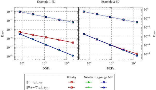
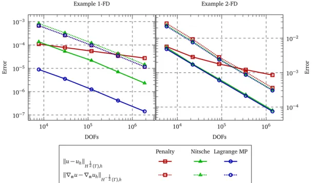
multiplier space due to the vital vertex method. . . 28 2.4 Different type of nodes characterized by the vital-vertex algorithm. 30 2.5 Discretization error in L2_{-norm and H}1_{-seminorm for the different}

methods applied to Example 1-FD and Example 2-FD. . . 33 2.6 Discretization error on the boundary, the error of the function in

H12_{(Γ ), h-norm and flux in H}−12_{(Γ ), h-norm for different methods}

applied to Example 1-FD and Example 2-FD. . . 34 2.7 The condition numbers of the stiffness matrices A arising from

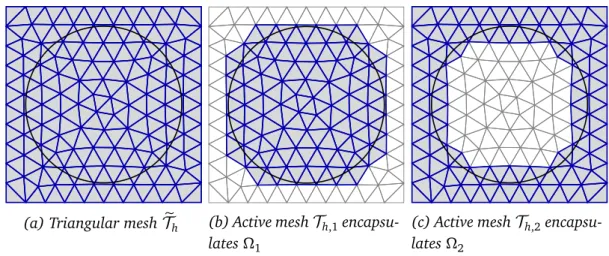
different methods against the number of DOFs, for Example 1-FD and Example 2-FD. . . 35 3.1 2D Triangular mesh is divided into two parts _Th,1 and Th,2 as

de-picted in (b) and (c) due to the interface Γ , elements which belong to the respective domain are shaded. . . 40 3.2 Discretization error in L2_{-norm and mesh-dependent energy norm}

(except for FEM formulation, where we use H1_{-seminorm) for}

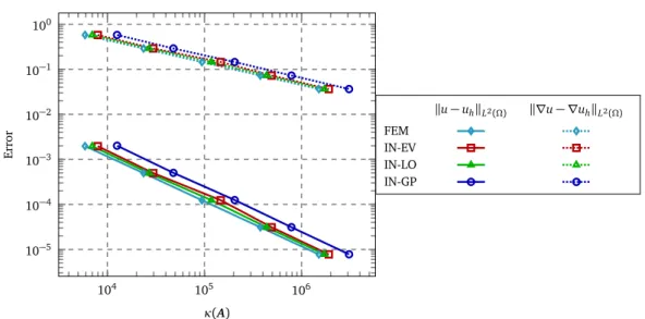
dif-ferent variants of Nitsche’s method applied to Example 1-IF. . . . 51 3.3 Discretization error in L2_{-norm and H}1_{-seminorm in the domain}

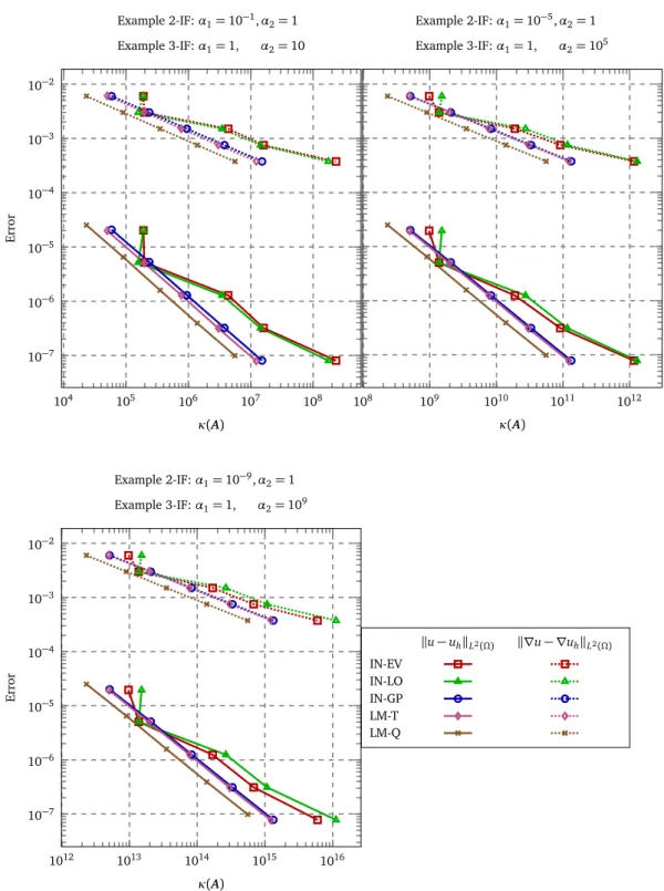
Ω for different methods applied to Example 2-IF and Example 3-IF. 52

3.4 Discretization error of the function in H12_{(Γ ), h-norm and flux in}

H−12_{(Γ ), h-norm for different methods applied to Example 2-IF and}

Example 3-IF. . . 53 4.1 A multigrid V (ν1, ν2)-cycle, where ν1and ν2denote number of

pre-smoothing and post-pre-smoothing steps. On the right, we can see a hierarchy of meshes associated with each level. . . 64

(18)

xvi Figures

4.2 2D Triangular meshes on different levels encapsulating the do-main Ωi, (domain Ωi is shaded in gray). . . 67

4.3 Basis of the cut domain in 1D, in blue we see the original basis VL,i 6⊃VL−1,i 6⊃VL−2,i, in red we see the basis computed with L2

-projections which are nested,_X_L,i_⊃_X_L−1,i_⊃_X_L−2,i. . . 68 4.4 Lagrange basis functions (in blue) for the cut domain and

corre-sponding biorthogonal basis functions (in red), the biorthogonal basis for the cut-element have been modified to satisfy biorthogo-nality condition for truncated support. . . 74 6.1 Signorini’s problem. . . 107 6.2 Two body contact problem. . . 111 6.3 Setup of the Signorini’s problem for experiments, the object in the

gray scale is the rigid obstacle. We can see the active background mesh and the displacement field. . . 119 6.4 Resultant displacement field and stress field of Signorini’s problem

Example 1-SC. . . 120 6.5 Resultant displacement field and stress field, as a solution of the

two-body contact problem, Example 1-TC, with Young’s modulus

E1= E2= 10, where the domain Ω2 is the circle. . . 122

6.6 Resultant displacement field and stress field, as a solution of the two-body contact problem, Example 2-TC, with Young’s modulus

E₁_{= 50 and E}₂_{= 10, where the domain Ω}₂ is the ellipse. . . 124 B.1 Splitting of a triangular element with the XFEM enrichments. . . . 130 B.2 Mapping the quadrature points on the enriched elements, the gray

region represents the region where support of the basis function is nonzero. . . 131 B.3 Mapping the quadrature points on the interface segment ΓK. . . . 131

B.4 Mapping the quadrature points on the intersection between the enriched elements from different levels. . . 132

(19)

Tables

2.1 The multilevel hierarchy of meshes with quadrilateral elements, with total number of active DOFs and number of active elements on a given level. . . 32 3.1 The multilevel hierarchy of meshes with triangular elements, with

total number of DOFs and number of elements on a given level. . 48 4.1 The number of iterations required by different solution methods to

reach the predefined tolerance, the last column shows the asymp-totic convergence rates of the SMG method. . . 77 4.2 The number of iterations required by the PCG-SMG method to

reach a predefined tolerance with a different number of levels in the multigrid hierarchy for solving Example 3-IF. . . 79 4.3 The number of iterations required by the PCG-SMG method to

reach a predefined tolerance for solving the problem with multiple interfaces in the domain. . . 79 5.1 The number of iterations required by CG and PCG methods to

reach a predefined tolerance for solving the Schur Complement system arising from Example 1-FD. In bracket, we have the total number of SMG iterations for solving the primal problem. . . 99 5.2 The number of iterations required by Uzawa-CG and Uzawa-PCG

methods to reach a predefined tolerance for solving the saddle point problem arising from Example 1-FD. In bracket, we have the total number of SMG iterations for solving the primal problem. 99 5.3 The number of iterations required by the projected CG method

(with various projection operators) to reach a predefined toler-ance for solving the saddle point problem arising from Example 1-FD. . . 100

(20)

xviii Tables

5.4 The number of iterations required by the generalized multigrid method to reach a predefined tolerance for solving the saddle point problem arising from the fictitious domain method. . . 102 5.5 The number of iterations required by the generalized multigrid

method to reach a predefined tolerance for solving the saddle point problem arising from the interface problem. . . 102 6.1 The number of iterations required by the generalized multigrid

method to reach a predefined tolerance for solving Signorini’s prob-lems (with two different kind of obstacles). . . 118 6.2 The number of iterations required by the generalized multigrid

method to reach a predefined tolerance for solving two-body con-tact problems. . . 123

(21)

List of Algorithms

4.1 Parallel Subspace Correction Iteration . . . 59

4.2 Successive Subspace Correction Iteration . . . 60

4.3 Two-grid Method . . . 63

4.4 Setup Semi-geometric Multigrid algorithm . . . 70

4.5 Semi-geometric Multigrid algorithm . . . 71

5.1 Conjugate projected gradient method . . . 90

5.2 Projected Gauss-Seidel method . . . 94

5.3 Generalized Multigrid algorithm . . . 95

5.4 Coarse level cycle . . . 96

C.1 Uzawa-Conjugate Gradient Method . . . 133

C.2 Uzawa-Preconditioned Conjugate Gradient Method . . . 134

(22)

(23)

Chapter 1 Introduction

In the last two decades, unfitted finite element methods have become quite popular. An unfitted method can be defined as any method where the com-putational domain does not match the mesh exactly. The rise in the popular-ity of the unfitted method is due to the fact that the finite element method (FEM) [BS07, Bra07, LB13] poses certain challenges for modeling problems on the complex domains or for problems with static or dynamic discontinuities. For modeling the problems on complex domains, it is essential to generate a mesh that could explicitly represent the computational domain. While for the prob-lems with a static discontinuity, it becomes essential to create a mesh, such that a discontinuity is resolved by the mesh. Whereas, for the problems with the dy-namic discontinuities, it would become necessary to adapt the mesh over time as the discontinuity evolves. In many of these cases, it can be a cumbersome, time-consuming, and computationally demanding task to create high-quality meshes, and failing to do so can result in usually sub-optimal approximation properties of FEM. Geometrically unfitted methods overcome these problems, as they just re-quire a background mesh and a finite element space defined on the background mesh. Clearly, the latter has to be modified to enforce the boundary conditions or the interface conditions. Here, an interface can be described as codimension one entity embedded in the domain, across which a function may exhibit non-smooth properties.

There is a huge variety of unfitted methods. The fictitious domain method can be listed as one of the oldest variants of an unfitted method [GPP94]. Later, Babuška and Melenk introduced the partition of unity finite element method which falls in the category of the meshless methods, as the meshes in the classical sense were not required [MB96, BM97]. Based on that work, Be-lytschko and Black proposed the idea of modeling crack propagation problems

(24)

2

with minimal remeshing of the finite element mesh, where the nodes near the crack surfaces and the crack tip were enriched to describe the crack [BB99]. This work was extended by Moës et al. by introducing the Heaviside func-tion and crack-tip funcfunc-tion, and this new method is termed as eXtended Fi-nite Element Method (XFEM) [MDB99]. Later, it was applied to the problems with the voids and inclusions by employing different types of enrichment func-tions [SCMB01, DMD+_{00]. Simultaneously, a similar approach to solve the}

in-terface problems without the need of remeshing was considered by Hansbo and Hansbo [HH02, HH04]. The methodology to enrich the background mesh used by Hansbo and Hansbo is very similar to the XFEM method introduced by Moës et al. [MCCR03], where the Heaviside functions are used with absolute shifted enrichments. In the work of Hansbo and Hansbo [HH02], in addition to the en-richments, Nitsche’s method was utilized to enforce the interface conditions in the unfitted finite element framework. A similar XFEM approach is also consid-ered for the two-phase flow problems in fluid dynamics to enrich the pressure variable [GRR06, Reu08, GR11]. Even though the XFEM has been introduced for problems in fracture mechanics with crack propagation, it has been later ap-plied to many different problems [FB10, MDS17]. In addition to the interface problems, the unfitted methods have been widely applied in the context of fic-titious domain methods [BH10, BH12, BH14]. The Finite Cell Method (FCM) can be considered as an extension of the fictitious domain method to higher-order function space [PDR07, SR15]. The FCM has been recently extended by employing the spline-based finite elements for harmonic and bi-harmonic problems [EDH10]. Another examples of unfitted methods can be given as the CutFEM method [BCH+_{15, CBM15], which normally emoploys a form of}

ghost penalty term to imporve the stability [Bur10]. In addition to these ods, we can also list other unfitted methods as the immersed boundary meth-ods [Pes02, SDS+_{12], immersogeometric analysis [KHS}+_{15], the trace finite}

ele-ment method [OR17], etc.

In the unfitted methods, a background mesh captures the computational do-main of arbitrary shape, thus the elements are allowed to be cut arbitrarily by the boundaries or interfaces. This could give rise to a highly ill-conditioned system of linear equations. Due to this reason, it becomes essential to develop efficient solution strategies or the preconditioning strategies for solving the linear systems arising from the unfitted discretization methods. Tailored preconditioning meth-ods for solving the interface problems with Nitsche based XFEM discretization were proposed and studied in [LMDM14, LR17, GLOR16].

In this work, we focus on developing the robust multilevel solution and preconditioning strategies in the unfitted finite element framework. Multilevel

(25)

3 1.1 Overview

methods are ideal iterative solvers for many large-scale linear/nonlinear prob-lems, as they are of optimal complexity [Hac86, TOS00, BvEHM00]. The opti-mal complexity implies that the convergence rate of the multilevel methods is bounded independently from the size of the problem, and the amount of numer-ical operations done in the algorithm is proportional to the size of the problem. The robustness of multilevel iteration results from a sophisticated combination of smoothing iterations and coarse level corrections. Ideally, these components are complementary to each other as they reduce errors in different parts of the spectrum. Traditionally, the mesh hierarchy for multilevel methods is created by either coarsening or refinement strategies, and a simple interpolation operator and its adjoint are used to transfer the information between different levels.

There have been some efforts to develop multilevel solution strategies for the XFEM discretization. Initial approaches propose to modify the algebraic multi-grid method (AMG). A domain decomposition-based AMG preconditioner is pro-posed for the fracture problems [BVWH+_{12], where the domain is decomposed}

into ‘cracked’ and ‘intact’ domain and AMG is applied to the ‘intact’ domain, and the ‘cracked’ domain is solved with a direct solver. Another approach using AMG for the XFEM discretization for the fracture problems is exploited in [GT13]. In an alternative approach, known as a quasi-algebraic multigrid method, the spar-sity pattern of the interpolation operator is modified to prevent the interpolation across the interfaces [HTW+_{12]. Recently, a new multigrid method is also}

pro-posed for the elliptic interface problems, with an interface smoother in [lud20].

1.1 Overview

The main objective of this thesis is to develop efficient multilevel methods for solving the optimization problems arising from the unfitted finite element dis-cretizations.

We start our discussion with a presentation of the discretization framework for the unfitted FEM. We introduce the XFEM with first-order finite element spaces for discretizing the fictitious domain and the interface problems. Here, we focus on the strategies for enforcing the boundary conditions and the interface conditions in the unfitted FEM framework. To enforce the boundary/interface conditions in a weak sense, we utilize the penalty method, Nitsche’s method, and the method of Lagrange multipliers. Next, we discuss in detail the numerical challenges posed by each method and evaluate the robustness of these methods by comparing their discretization errors and the condition numbers of arising linear systems.

(26)

4 1.1 Overview

Then, we propose tailored multigrid methods for solving the system of equa-tions arising from Nitsche’s method and the method of Lagrange multipliers. The multigrid method requires transfer operators to transfer the information between the mesh hierarchy. In the unfitted framework, the mesh hierarchy is generally created by the either coarsening or refinement of the background meshes. Thus, even though the background meshes are nested, the meshes associated with the computational domain may not be nested. Hence, we propose a new transfer operator for the unfitted meshes computed using L2_{-projection and pseudo-L}2

-projection [DK11, DK14, KK19]. Additionally, the system of equations arising from the method of Lagrange multipliers has a saddle point structure, which can also be formulated as a quadratic minimization problem with linear equality constraints. Here, we introduce a new generalized multigrid method for solving such problems. This generalized multigrid method is an extension of the mono-tone multigrid method [Kor94, Kor96, KK01], which was introduced for solving quadratic minimization problems with pointwise constraints.

As a culmination of this thesis, we employ the unfitted finite element methods for solving contact problems. We use the method of Lagrange multipliers to dis-cretize the non-penetration condition for contact problems. In addition, we use our novel generalized multigrid method for solving the quadratic minimization problems with linear inequality constraints.

Here, we provide a brief list of the contributions made in this thesis:

• We compare the penalty method, Nitsche’s method, and the method of La-grange multipliers used for enforcing the boundary/interface conditions. We evaluate the performance of these methods by comparing their dis-cretization errors and condition numbers of the linear system by means of several numerical examples.

• We introduce a new transfer operator in the unfitted framework. We eval-uate the robustness of this transfer operator by employing it in the semi-geometric multigrid method for solving the linear systems, which arise from fictitious domain method and interface problems when using the penalty method or Nitsche’s method.

• We evaluate the performance of the standard iterative methods for solving the saddle point problems that arise due to the method of Lagrange mul-tipliers. We also assess the performance of the semi-geometric multigrid method as a solution strategy for solving the primal problem.

• We introduce a generalized multigrid method for solving the saddle point problem, or an equivalent quadratic minimization problem with linear

(27)

con-5 1.2 Function Spaces

straints, arising from the method of Lagrange multipliers. In order to han-dle the linear constraints, we propose a technique to decouple the con-straints and introduce a variant of the projected Gauss-Seidel method. • Finally, we employ all these ingredients for solving the contact problem

in the unfitted framework. We use the method of Lagrange multipliers to enforce the non-penetration conditions for Signorini’s problem and two-body contact problems. In the end, we extend the generalized multigrid method for solving contact problems.

1.2 Function Spaces

In this work, we discuss the finite element method for solving the second-order partial differential equations. The Sobolev spaces are a natural choice for the variational problems of this kind. Here, we give an introduction to the notations used in this work and later give a short description of the Sobolev spaces. For the detailed review of the Sobolev spaces, we refer to the monographs [BS07, Bra07, Sal08].

Notations: In this work, the scalar quantities, such as functions, constants, op-erators are denoted by lower case and upper case characters e.g., u, v, f , C. The vector quantities are denoted by bold symbols in lower case characters e.g., a, b, and the matrix quantities are denoted by bold symbols in upper case characters e.g., A, B. We denote a matrix A ∈ Rm×n_{, where the symbols R}m×n _{denote the}

set of m × n matrices with real entries. For a given matrix A, its transpose is de-noted by AT_{. The components of these vector and matrix quantities are given as}

ai, bj, Ai j, Bkl for some indices i, j, k, l. By symbolsV,W, we denote real normed

function spaces. Given a function space _V, we denote its dual space that con-tains all bounded linear functionals by_V∗_{. We denote the vector-valued function}

spaces by V = (V)d, where d ∈ {2, 3}.

The Euclidean inner product is defined as u · v := Piuivi for u, v ∈ Rn. We

define scalar energy product (·, ·)A as (u, v)A := u · Av, for all u, v ∈ Rn and

the induced energy norm is defined as k · k2

A:= (·, ·)A. Additionally, we define the

Kronecker delta δi j for some indices i, j by

δ_{i j} ₌¨1 if i = j,

(28)

6 1.2 Function Spaces

Sobolev Spaces: We consider a simple and connected domain Ω ⊂ Rd for

d ∈ {2, 3}. The domain Ω is an open and bounded in the Euclidean space with

Lipschitz boundary ∂ Ω and the outer normal vector from the domain is defined as

n. We assume, the boundary ∂ Ω can be decomposed into two subsets; the closed

Dirichlet boundary ∂ Ω_D and the open Neumann boundary ∂ Ω_N, such that

∂ ΩD∪ ∂ ΩN= ∂ Ω and ∂ ΩD∩ ∂ ΩN = ;.

We denote the elements of Ω by x = (x1, x2, . . . , xd). On the domain Ω, a scalar

valued function is defined as u : Ω → R and a vector valued function is defined as v : Ω → Rd_.

We define a multi-index as a d-tuple a = (a1, a2, . . . , ad), ∀ai ∈ N. The length

of a multi-index is given by |a| := P_1¶i¶da_i. The a-th derivative of order |a| is denoted by ∂a₌ ∂ a1 ∂ xa1 1 ∂a2 ∂ xa2 2 · · · ∂ad ∂ xad d . Let L2

(Ω) be a Lebesgue space of square-integrable function on the domain

Ω. The inner product on L2_{(Ω) is denoted as (u, v)}_L2_(Ω) := R

Ωu(x)v(x) dΩ,

and the induced L2_{-norm is defined as k · k}2

L2_(Ω) := (·, ·)L2_(Ω). The

sym-bol L∞_{(Ω) denotes the space of essentially bounded function with norm}

kvkL∞_(Ω):= ess sup_{x ∈Ω}|v(x)|.

Additionally, by Hk

(Ω), we denote the Sobolev space of function with k ¾ 0 square-integrable weak derivatives on the domain Ω. We note, L2

(Ω) = H0(Ω). Then ∂a _{denotes the weak differentiation and the corresponding norm in H}k_(Ω)

are given as kvk2Hk_(Ω):= kvk2_L2_(Ω)+ X 1¶|a|¶k k∂avk2 L2_(Ω). The space Hk

(Ω) is a Hilbert space with respect to the scalar product (u, v)Hk_(Ω)= (u, v)_L2_(Ω)+

X

1¶|a|¶k

(∂au, ∂av)L2_(Ω).

In this work, we use several subspaces of H1

(Ω) and L2(Ω). We denote the sub-space of H1

(Ω) with all the function that vanish on the Dirichlet boundary ∂ ΩD

is denoted as H1

D(Ω), we have

H1

D(Ω) = {v ∈ H1(Ω) : v|∂ ΩD = 0},

and if the whole boundary is Dirichlet boundary ∂ Ω_D_{= ∂ Ω, we have}

H1

(29)

7 1.3 Outline

When the boundary ∂ Ω is Lipschitz continuous, we introduce a linear and continuous operator

γ₀_{(·) : H}1_{(Ω) → H}12_{(∂ Ω).}

The operator γ0 is surjective and it is known as a trace operator. For simplicity,

we denote the restriction of a function u on the boundary ∂ Ω by u|∂ Ω. Given

u ∈ H1

(Ω), the image of the trace operator γ0(u) coincides with the restriction

of u to the boundary ∂ Ω, given as γ0(u) = u|∂ Ω, which we refer to as trace of u

on the boundary ∂ Ω. In addition, the dual of the space of H12_{(∂ Ω) is denoted as}

H−12_{(∂ Ω), and the duality paring between these two spaces is given as}

〈·, ·〉∂ Ω: H−

1

2_{(∂ Ω) × H}12_{(∂ Ω) → R.}

1.3 Outline

This thesis is organized as follows.

• In Chapter 2, we introduce the fictitious domain method in the unfitted finite element framework. We introduce the penalty method, Nitsche’s method, and the method of Lagrange multipliers for enforcing the Dirichlet boundary conditions. Also, we review various approaches for estimating the value of the stabilization parameter used in Nitsche’s method. In ad-dition, we also discuss the necessity of satisfying the inf-sup condition and introduce the vital vertex algorithm to construct a stable multiplier space. • In Chapter 3, we introduce the interface problem as overlapping fictitious domains in the XFEM framework. Our presentation is given as an extension of Nitsche’s method and the method of Lagrange multipliers from enforcing boundary conditions to enforcing interface conditions.

• In Chapter 4, we review the multigrid method as subspace correction method. Later, we introduce the multilevel framework for creating a nested hierarchy of the FE space from a hierarchy of the background meshes. We present the variational transfer approach to compute the transfer operators by means of L2_{-projections and pseudo-L}2_{-projections.}

• In Chapter 5, we discuss standard iterative methods for solving saddle point problems and review some preconditioners for the dual systems. Then, we introduce the generalized multigrid method for solving the quadratic minimization problem with linear equality constraints.

(30)

8 1.3 Outline

• In Chapter 6, we introduce contact problems in the unfitted framework. We use the method of Lagrange multipliers for imposing the non-penetration condition on the unfitted interface and we use our generalized multigrid method for solving the contact problems.

(31)

Chapter 2 Fictitious Domain Method

The fictitious domain method is among one of the earliest variants of unfitted methods [GPP94, GG95]. This method was introduced to simplify the process of numerically solving partial differential equations on complex domains using reg-ular structured meshes. In this approach, the solution of the problem is defined only up to the boundary of the computational domain. Thus, the weak formula-tion of a problem is defined only on the elements that are located in the interior of the domain. This method is a subset of a Galerkin method, and it inherits the approximation properties of the standard finite element methods.

The unfitted method simplifies the task of creating high-quality meshes that fit the domains, but it gives rise to some other challenges. Firstly, we have to store various details about the actual computational domain and identify the part of the background mesh that is associated with the domain. Secondly, we have to pay attention to the numerical integration of the elements that are intersected by the boundary and are only partially inside of the domain. The last challenge is concerning the imposition of the Dirichlet boundary conditions. As the boundary of the computational domain does not fit the background mesh exactly, we have to enforce the Dirichlet boundary conditions in a weak sense.

In this chapter, we provide an introduction to the fictitious domain method in the extended finite element framework and discuss various methods to enforce the boundary conditions. The concepts outlined in this chapter are extended in the next chapter for tackling the interface problems. Additionally, in order to highlight elements of the discretization method, we limit our presentation in this chapter to a model diffusion problem.

In Section 2.1, we define a diffusion problem on a domain Ω. The assump-tions on the background mesh and the finite element function spaces are dis-cussed in Section 2.2. In Section 2.3, we give a weak formulation of the

(32)

10 2.1 Model Problem

sion problem and pose the problem in an optimization framework with Dirichlet boundary conditions as constraints. Further, we investigate different strategies to enforce the Dirichlet boundary conditions in the XFEM framework, e.g., the penalty method, the method of Lagrange multipliers, and Nitsche’s method in Section 2.4. Later, we discuss the stabilization parameter in Nitsche’s method which plays an important role in establishing the coercivity of the bilinear form. In Section 2.5, we discuss strategies to implicitly estimate the value of the stabi-lization parameter. Then, we discuss a method to create a stable space for the Lagrange multipliers in Section 2.6. In the last section, we perform some nu-merical experiments to show the convergence properties of the penalty method, Nitsche’s method, and the method of Lagrange multipliers for different test ex-amples.

2.1 Model Problem

We assume a bounded domain Ω ⊂ Rd_{, d ∈ {2, 3} with the boundary ∂ Ω. In this}

section, we denote the boundary as Γ := ∂ Ω. The boundary Γ is assumed to be Lipschitz continuous. We consider the following diffusion problem as a model problem.

Given the data f ∈ L2

(Ω) and a function gD∈ H

1

2_{(Γ ), find a function u such}

that

−∇ · α(x)∇u = f in Ω,

u = gD on Γ ,

(2.1) where the coefficient α : Ω → R+ _{is piecewise constant satisfying}

α(x ) ¾ α0> 0.

With a slight abuse of notation, we write α = α(x). The model problem (2.1) has a unique solution u ∈ H1_{(Ω) that satisfies}

kukH1_(Ω)_{¶ C}(k f k_L2_(Ω)+ kg_Dk

H12_{(Γ )}).

The weak formulation of the problem (2.1), which has inhomogeneous Dirichlet boundary conditions, is given as, find u ∈ H1

0(Ω) such that

(α∇u, ∇v)L2_(Ω) = ( f , v)_L2_(Ω)− (α∇u_g, ∇v)_L2_(Ω) ∀v ∈ H₀1(Ω), (2.2)

where u_g_{∈ H}1

(33)

11 2.2 Finite Element Discretization

We remark that the formulation (2.2) is equivalent to the following minimiza-tion problem. Find u ∈ H1

0(Ω) such that

min

u∈H1_0(Ω)

1

2(α∇(u + ug), ∇u)L2(Ω)− (f , u)L2_(Ω). (2.3)

In both of the above formulations (2.2) and (2.3), the solution is sought in the

H1

0(Ω) space.

2.2 Finite Element Discretization

In the previous section, the weak formulation is still given in a continuous sense. In this section, we introduce the necessary ingredients for the discretization of the diffusion problem in the extended finite element framework.

2.2.1 Background Mesh

We assume a domain D, that encapsulates the computational domain Ω, i.e.,

Ω ⊂ D. We define shape regular, quasi-uniform, conforming triangulation on

the background domain. The partition of the background domain D is given by simplicies Ki∈ Rd such that

Dh= {K1, K2, . . .}.

Now, we can define the closure of the background domain as union of closure of all simplicies, given as

Dh= {K1, K2, . . .} = ∪K∈DhK.

The background triangulation which is associated with our domain is defined as follows:

e

Th= Dh\∂ Dh.

The domain Ω is encapsulated by the mesh, Ω ⊂ eTh, but the mesh is not fitted to

the boundary of the domain. The boundary of the domain is resolved sufficiently well by the meshTe_h and the curvature of the boundary is bounded.

We useTe_h as a background triangulation which captures the domain. Let h_K be the diameter of the element K, and mesh size is defined as h = max_{K∈ e}_ThhK.

We define so-called active mesh, which is strictly intersected by the domain Ω as Th= {K ∈ eTh: K ∩ Ω 6= ;}.

(34)

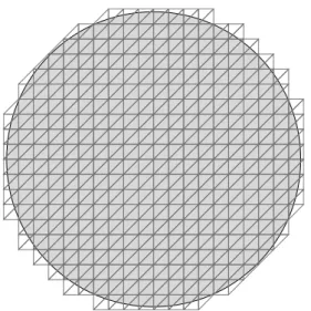
The active mesh_T_hexcludes all the elements that are neither intersected by the boundary Γ nor are in the interior of the domain. In Figures (2.1a, 2.1b), we can see an example of a background meshTe_hand an active meshT_hthat encapsulates a circular domain.

We define a set of elements that are intersected by the boundary Γ as Th,Γ = {K ∈ eTh: K ∩ Γ 6= ;}.

For all elements K ∈Th,Γ, let KΩ:= K ∩ Ω be part of K in domain Ω. While for all

elements K ∈ Th\Th,Γ are strictly in the interior of domain Ω. For all K ∈ Th,Γ,

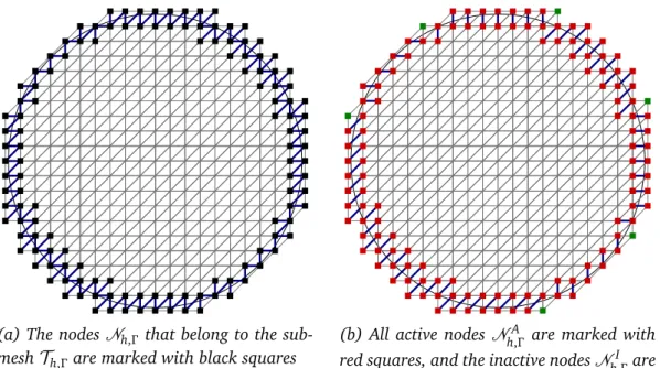
let ΓK := Γ ∩ K be part of Γ in K. Additionally, we define the set of facesGh,Γ

Gh,Γ = {G ⊂ ∂ K : ∂ K ∩ ∂Th= ;, ∀K ∈Th,Γ}.

This set includes all the faces that are associated with the cut elements, except the ones that are on the boundary of the mesh ∂_Th. In Figure 2.1c, we can see the

distinction between the elements of mesh_Th,Γ and the elements of meshTh\Th,Γ.

While in Figure 2.1d we can see the set of faces that belong to the set _Gh,Γ.

2.2.2 Extended Finite Element Space

We define a continuous first order finite element (FE) space over the triangulation e

Th as

e

Vh= {v ∈ H1( eTh) : v|K ∈P1(K), ∀K ∈ eTh},

where_P1 denotes the space of piecewise linear functions. Following the original

XFEM literature [MDB99], we define a characteristic function of the computa-tional domain Ω, given as

χ_Ω: Rd _{→ R,} χ_Ω_{(x ) =}¨1 ∀x ∈ Ω,

0 otherwise. (2.4)

The characteristic function is used to restrict the support of the finite element space Ve_h to the domain Ω. Thus, the space of finite elements in the domain Ω is defined as

Vh = χΩ(x ) eVh. (2.5)

We obtain the “cut” basis associated with a node p as,

(35)

(a) A triangular meshTe_his used as a

back-ground mesh to capture a circular domain Ω.

(b) the mesh_This strictly intersected by the

domain Ω.

(c) The mesh _T_h,Γ is shaded in blue, while the interior mesh_T_h_\_T_h,Γis shaded in green.

(d) The set of faces_G_h,Γis shown in the red. Figure 2.1. An example of a domain Ω with a background meshTe_h.

(36)

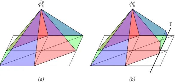
14 2.3 Variational Formulation ˜ φ_hp (a) Γ φ_hp (b) Figure 2.2. (a) The basis functionφe

p

h associated with a node p, (b) The “cut” basis

function φ_hp= χΩi(x ) eφ

p

h associated with the node p

Here, Nfh denotes the set of nodes of the active meshTe_h. Now, the set of nodes associated with the domain Ω can be given as

Nh= {p ∈ fNh: supp(φhp) ∩ Ω 6= ;}.

The FE space_Vhis spanned by the nodal basis functions given as, Φh= (φhp)p∈Nh.

In Figure 2.2, we can see the basis functionφe

p

h associated with the original

func-tion space Ve_h and corresponding cut basis function φ

p

h associated with the FE

space _V_h.

2.3 Variational Formulation

Now, we discretize the problem (2.1) using the FE space _Vh defined on the

ac-tive mesh _Th. We write the discretized variational formulation of the diffusion

problem (2.1) as a constrained minimization problem. Find uh∈Vh such that

min uh∈Vh J(uh) = 1 2a(uh, uh) − F(uh) subject to uh= gD on Γ , (2.6)

where J(·) : Vh → R denotes the energy functional, a(·, ·) : Vh×Vh → R is a

(37)

15 2.3 Variational Formulation

continuous linear form. The bilinear and the linear forms are defined as

a(uh, vh) := (α∇uh, ∇vh)L2_(Ω),

F(vh) := ( f , vh)L2_(Ω).

We remark that the formulation (2.3) is posed as an unconstrained minimization problem, while (2.6) is formulated as a constrained minimization problem. In the unfitted finite element framework, it is not possible to impose the Dirich-let boundary condition in a pointwise manner as the mesh is not fitted to the boundary of the domain. Thus, we have to rely on other methods to impose the Dirichlet boundary conditions in a weak manner. We also mention that, we seek the solution of (2.3) in H1

0(Ω) space while for (2.6) the solution is sought in a

larger space _Vh⊆ H1(Ω).

Before discussing the weak formulation in the XFEM framework we need to define the appropriate norms. We define mesh-dependent inner products on the boundary as (u, v)_H1 2_{(Γ ),h}:= X K∈Th,Γ (h−1K u, v)L2_(Γ K), (u, v)_H− 12_{(Γ ),h}:= X K∈Th,Γ (hKu, v)L2_(Γ_K₎.

The induced mesh-dependent norms at the boundary are given as

kvk2 H12_{(Γ ),h}= X K∈Th,Γ 1 h_K kvk 2 L2_(Γ K), kvk2 H− 12_{(Γ ),h}= X K∈Th,Γ h_K_kvk2 L2_(Γ_K_). (2.7) We recall, 〈·, ·〉Γ : H− 1

2_{(Γ )×H}12_{(Γ ) → R, denotes a duality paring on the boundary.}

On the duality pairing, we have the following inequality due to Cauchy-Schwarz 〈u, v〉Γ ¶kuk_H− 12_{(Γ ),h}kvkH12_{(Γ ),h}. (2.8)

For the FE space _Vh an important trace inequality on each element K ∈ Th,Γ is

given as kα∇nuhk2 H− 12(ΓK),h¶ Cγkα 1 2∇u hk2L2_(K Ω), (2.9)

where, ∇nu = n · ∇u. Here, we note that the constant Cγ depends on the shape

(38)

16 2.3 Variational Formulation

2.3.1 Causes of Ill-conditioning

In the unfitted methods, a background mesh captures the computational domain of arbitrary shape, hence the elements are allowed to be cut arbitrarily by the boundary. In general, this flexibility can result in disproportionally cut elements that might not be shape regular anymore. For an element K ∈ Th, the bound

on the gradient of a function is established by the following inverse inequality relation

k∇uhkL2_(K)_{¶ C h}−1_K ku_hk_L2_(K), (2.10)

where, the constant C depends on the shape regularity of element K. Now, for the cut elements, ∀ K ∈ Th,Γ, the constant C depends on the shape regularity

of element K_Ω and on the mesh size of the element h_K, which can become arbi-trarily small. Therefore, the bounds on the gradients of the function can become arbitrarily weak depending on the location of the boundary with respect to the background mesh. The inverse inequality relation (2.10) is necessary to provide the bounds for the condition number estimates of the system matrix, hence a large value of the constant C in the above inequality gives rise to linear systems of equation with large condition numbers. Indirectly, the condition number of the system matrix depends on the cut position and the conditioning of the lin-ear system may become arbitrarily poor when an interface passes very close to element faces or nodes. In order to tackle the issue of poor conditioning of the system matrix, the ghost penalty method was introduced.

2.3.2 Ghost Penalty Stabilization

In this section, we introduce a new stabilization term, called the ghost penalty, in the variational formulation. The ghost penalty term was introduced to recover the control over the gradients of the function on the cut elements [Bur10]. The ghost penalty method was introduced in the context of Nitsche’s method to im-prove the robustness of the method irrespective of the location of the bound-ary [BH12, Bur10]. The idea of such a stabilization term was used for the problems with dominant transport to penalize the jumps in the normal deriva-tive across the interior faces of elements [DD76]. This type of penalty term was recently also applied in the context of convection-diffusion-reaction prob-lem [BH04], Stoke’s probprob-lem [BH06] and in the XFEM context for incompressible elasticity problems to penalize the jump in pressure [BBH09].

The ghost penalty term consists of a least-square penalization of the flux jumps across the element boundaries, which weakly enforces the continuity of normal flux at the element interfaces in the neighborhood of the boundary. This

(39)

17 2.4 Enforcing Boundary Conditions

penalty term has to be chosen in such a way that it provides sufficient stability and it stays weakly consistent with the original formulation for smooth solutions. The ghost penalty term is enforced on the set of faces _Gh,Γ, and it is defined as

g(uh, vh) =

X

G∈Gh,Γ

ε_Gh_G_α(_J∇_n_G_E_hu_h_{K, J∇}_n_G_E_hv_h_K)_L2_(G), _(2.11)

where h_Gis the diameter of face G, n_Gdenotes unit normal to face G, and ε_Gis a positive constant. Here,_Eh denotes the canonical extension of the function from

the domain to the background mesh, which is defined as_Eh:Vh|KΩ → eVh|K.

By adding the ghost penalty term, we regain the control over the gradients of the function on the cut elements with very small support and by extension we overcome the issue of ill-conditioning. The coercivity of the bilinear form a(·, ·) in the discrete sense is defined only up to the boundary of the computational domain. Adding the stabilization term to the bilinear form a(·, ·) extends the coercivity from the computational domain to the active mesh,

a(vh, vh) + g(vh, vh) ¾ Cs

X

K∈Th

kα12∇v

hk2L2_(K).

In [Bur10], it is shown that the extended coercivity is enough to ensure a uni-form upper bound on the condition number of the system matrix. The condition number of the system matrix associated with the updated bilinear form does not depend on the location of the boundary with respect to the background mesh.

Even though, the ghost penalty stabilization term was introduced in the con-text of Nitsche’s method, we add this term to the bilinear form regardless of the method chosen to enforce the Dirichlet boundary condition. We modify the energy formulation in (2.6), by introducing an additional ghost penalty stabi-lization term (2.11). The modified energy functional is given as

J(uh) := 1₂

a(uh, uh) + g(uh, uh)

− F(uh). (2.12)

Since its introduction, the ghost penalty term has become quite popular in the unfitted finite element framework. The ghost penalty terms have been used for different variants of the unfitted finite element framework e.g., in so-called Cut-FEM methods[BCH+_{15], cut discontinuous Galerkin methods [GM18, GM19].}

2.4 Enforcing Boundary Conditions

In this section, we discuss different strategies for enforcing the Dirichlet bound-ary condition. We reformulate the problem (2.6) with the modified energy

(40)

func-18 2.4 Enforcing Boundary Conditions

tional (2.12) that includes the ghost penalty term. Thus, the updated minimiza-tion problem is given below. Find uh∈Vhsuch that

min uh∈Vh J(uh) = 1 2 a(uh, uh) + g(uh, uh) − F(uh) subject to u_h_{= g}_D on Γ . (2.13)

In this section, we consider a constrained optimization framework to derive a weak formulation of the above problem.

2.4.1 The Penalty Method

The idea of enforcing the Dirichlet boundary condition in the finite element framework in a weak sense dates back to the work of Babuška [Bab73b]. The penalty method is one of the simplest ways to recast an equality constrained min-imization problem to an unconstrained minmin-imization problem. This is done by adding an extra term to the energy functional which penalizes the violation of the constraints.

Here, we consider a quadratic penalty method that penalizes the constraints in a least squares sense. The modified energy functional is given as

min uh∈Vh JP(uh) := J(uh) + γ_p 2 kuh− gDk 2 H12_{(Γ ),h},

where γp ∈ R+ is the penalty parameter. If the penalty parameter is chosen to

be large enough, then the solution of the above minimization problem leads to a solution that satisfies the Dirichlet boundary condition approximately.

The Euler-Lagrange condition corresponding to the above minimization prob-lem yields:

find uh∈Vh such that AP(uh, vh) = FP(vh) ∀vh∈Vh. (2.14)

Here, the bilinear functional AP(·, ·) and the linear functional FP(·) are defined

as

A_P_(u_h, v_h_{) = a(u}_h, v_h_{) + g(u}_h, v_h_{) + (γ}_pu_h, v_h₎

H12_{(Γ ),h},

F_P_(v_h_{) = F(v}_h_{) + (γ}_pg_D, v_h₎_H1 2_{(Γ ),h}.

This formulation can be also achieved by reformulating the Dirichlet boundary condition to a Neumann or a Robin type condition and then using the Neumann boundary condition in the Green’s formula for the problem (2.1) [BE86].

(41)

Although the penalty method is trivial to implement, it is not widely used since it is not consistent with the strong formulation (2.1). The system matrix as-sociated with the bilinear functional AP(·, ·) can produce a highly ill-conditioned

system if a large penalty parameter is chosen. The convergence of the discretiza-tion error depends on the value of the penalty parameter. If a large enough penalty parameter is not chosen, the method may produce sub-optimal converge rates. Analysis of the penalty method for the fitted method is carried out in [Bab73b, BE86], but in our knowledge, the analysis for the penalty method in the unfitted finite element framework is not available.

2.4.2 The Method of Lagrange Multipliers

The method of Lagrange multipliers was also introduced by Babuška in the finite element framework to impose the Dirichlet boundary conditions [Bab73a]. It is also extensively used in the field of constrained optimization problems to en-force equality constraints. This method results in the mixed formulation which requires the solution of the primal variable and an additional multiplier.

We define a Lagrangian function_L(·, ·) :Vh×Mh→ R, whereMh is a

mul-tiplier space,_Mh⊆ H−

1

2_{(Γ ). The Lagrangian function for enforcing the Dirichlet}

boundary condition is defined as

L(uh, λh) = J(uh) + 〈λh, uh− gD〉Γ. (2.15)

The saddle-point (uh, λh) ∈Vh×Mh is the solution of the above problem given

as

L(uh, µh) ¶L(uh, λh) ¶L(vh, λh) ∀(vh, µh) ∈Vh×Mh.

The first order optimality conditions of the Lagrangian formulation (2.15) can be reformulated into the following equivalent formulation.

Find (uh, λh) ∈Vh×Mh such that

a(uh, vh) + g(uh, vh) + b(λh, vh) = F(vh) ∀vh ∈Vh,

b(µh, uh) = GD(µh) ∀µh∈Mh.

(2.16)

Here, the bilinear form b(·, ·) :Mh×Vh→ R and the linear form GD:Mh→ R

are defined as b(λh, uh) := X K∈Th,Γ 〈λh, uh〉ΓK and GD(λh) := X K∈Th,Γ 〈λh, gD〉ΓK.

The method of Lagrange multipliers is an attractive option for enforcing the Dirichlet boundary conditions. However, it is stable only if the following discrete

(42)

inf-sup condition is satisfied

inf λh∈Mh sup uh∈Vh b(λh, uh) kλhk_H_{− 12}_{(Γ ),h}kuhkH1_(Ω) ¾ β > 0, (2.17)

where the constant β does not depend on the mesh size h. The choice of a fi-nite element space for the Lagrange multiplier is very essential to have a stable discretization method. In the XFEM framework, most naive options for the pri-mal and the multiplier spaces do not satisfy the inf-sup sup condition. In the original work of the fictitious domain methods, the Lagrange multiplier method was used for imposing the Dirichlet boundary conditions [GPP94, GG95]. In that case, the primal variable and the Lagrange multiplier are discretized on two dif-ferent meshes. The Lagrange multiplier is discretized on a coarser mesh such that the mesh size of the coarse mesh is at least three times larger than the mesh chosen to discretize the primal variable [GPP94].

The inf-sup condition (2.17) can be circumvented by introducing additional stabilization terms. In the work of Barbosa and Hughes [BH91, BH92a], the inf-sup condition is avoided by adding a least-square penalty term that minimizes the difference between the multiplier and its physical interpretation. Their method is also introduced to the XFEM framework and analyzed in detail for the fictitious domain problem in [HR09].

We discuss stable discretization spaces for the Lagrange multiplier and ways to circumvent the inf-sup condition in more detail in Section 2.4.2.

2.4.3 Nitsche’s Method

Nitsche’s method was introduced as an alternative to the penalty method and the method of Lagrange multipliers to enforce the Dirichlet boundary condi-tions [Nit71]. This method is utilized in many different discretization meth-ods as it is simple to use. For example, in the discontinuous Galerkin (DG) method, Nitsche’s method is used to enforce the continuity between each ele-ment faces [Arn82]. It is also used in a domain decomposition methods to mor-tar the interfaces between non-matching meshes [BFMR97, BHS03]. Nitsche’s method is also a popular choice for enforcing the Dirichlet boundary conditions for mesh-free methods and particle methods [GS03].

This method can be regarded as a variationally consistent penalty method. An alternative interpretation of the method is as a stabilized Lagrange multiplier method, where the Lagrange multiplier is explicitly expressed by its physical in-terpretation as an outward flux in the primal variable [Ste95].

(43)

We start with an augmented Lagrangian functional_L_A_{(·, ·) :}_V_h_×_M_h _{→ R,} where the formulation is given as

LA(uh, λh) = J(uh) + 〈λh, uh− gD〉Γ +

γ_p

2 kuh− gDk2H12_{(Γ ),h}. (2.18)

If we solve this problem, the saddle-point point (uh, λh) ∈Vh×Mhis the solution

of the above problem given as

LA(uh, µh) ¶LA(uh, λh) ¶LA(vh, λh) ∀(vh, µh) ∈Vh×Mh.

But rather than solving for the saddle-point problem, we replace the Lagrange multiplier by its physical interpretation. In the context of problem (2.1) the Lagrange multiplier can be interpreted as outward flux at the boundary, given as

λh= −α∇nuh.

Using this information, we reformulate the augmented Lagrangian formulation (2.18) from mixed formulation to primal formulation. We define energy func-tional, JN(·) :Vh → R as JN(uh) :=LA(uh, −α∇nuh). The modified energy

func-tional is given as min uh∈Vh JN(uh) = J(uh) − 〈α∇nuh, uh− gD〉Γ+ γ_p 2 kuh− gDk 2 H12_{(Γ ),h}. (2.19)

This formulation can be referred to as the energy formulation of Nitsche’s method.

The first order optimality condition corresponding to the minimization prob-lem (2.19) yields the abstract variational probprob-lem.

Find uh∈Vh such that AN(uh, vh) = FN(vh) ∀vh∈Vh, (2.20)

where the bilinear from AN(·, ·) and the linear form FN(·) are defined as

AN(uh, vh) = a(uh, vh) + g(uh, vh) − 〈α∇nuh, vh〉Γ− 〈α∇nvh, uh〉Γ

+ (γpuh, vh)_H1 2_{(Γ ),h},

FN(vh) = F(vh) − 〈α∇nvh, gD〉Γ+ (γpgD, vh)_H12_{(Γ ),h}.

(2.21)

The connection between the Lagrange multiplier method of Barbosa-Hughes and Nitsche’s method is established in [Ste95]. Nitsche’s method can be regarded as a penalty method with extra consistency terms with the normal derivatives across the boundary.

(44)

22 2.5 Stabilization Parameter in Nitsche’s Method

Nitsche’s method was introduced in the unfitted finite element method in con-text of the interface problem to enforce the interface conditions [HH02]. Later, this work was extended to more generic problems and applied to the fictitious do-main problems [BH12]. Under reasonable mesh assumptions on the background mesh, a priori error estimates are given by [BH12],

|||u − uh|||h¶ C hkukH2_(Ω) ∀u ∈V_h,

ku − uhkL2_(Ω) _{¶ C h}2kuk_H2_(Ω) ∀u ∈V_h,

where the constant C is completely independent of the location of the interface in the mesh. The mesh-dependent energy norms |||·|||hin the above estimates are

defined as

|||v|||2h:= k∇vk2L2_(Ω)+ γpkvk2

H12_{(Γ ),h}+ k∇nvk 2

H− 12_{(Γ ),h}.

2.5 Stabilization Parameter in Nitsche’s Method

As mentioned in the previous section, Nitsche’s formulation is stable only if the bilinear form A_N_{(·, ·) is coercive, for example by choosing a sufficiently large} stabilization parameter γp. Estimation of such a stabilization parameter is a very

delicate task. If the value of the stabilization parameter is too large, it gives rise to an ill-conditioned system matrix. It becomes increasingly difficult to estimate the stabilization parameter for irregular meshes and higher-order finite elements. In this section, we explore different methods for estimating the stabilization parameter. Following the coercivity of the bilinear form (2.21), we have

AN(vh, vh) ¾ X K∈Th\Th,Γ kα12∇v hk2L2_(K)+ 1 εkα 1 2∇ nvhk2 H− 12(Γ ),h+ g(vh, vh) + X K∈Th,Γ 1 −2Cγ ε kα 1 2∇v hk2L2_(K Ω)+ (γp− ε)kvhk 2 H12_{(Γ ),h}.

This inequality utilizes Young’s inequality for some ε > 0 and follows trace in-equality (2.9) (see A.1). The bilinear form is coercive if the positivity of two terms in the last line is ensured, given by ε ¾ 2Cγ, and γp¾ ε. Thus, the stabilization

parameter can be given with the bound γp¾ 2Cγ.

The stabilization parameter thus influences two different aspects. Firstly, if the stabilization parameter has to be chosen sufficiently large such that the sta-bility of the method is insured. Secondly, we know that the large stabilization parameter enforces the Dirichlet boundary conditions more accurately. Hence, a large stabilization parameter reduces the discretization error at the boundary,

(45)

23 2.5 Stabilization Parameter in Nitsche’s Method

but simultaneously it increases the condition number of the linear system. Thus, it is necessary to strike a balance between the discretization error and the condi-tioning of the system. Therefore, we aim to choose the value of the stabilization parameter larger than the value required to ensure stability but not too large that the system matrix becomes poorly conditioned.

In the next sections, we discuss two approaches: the first one for estimating the stabilization parameter and the second one for circumventing the need to compute the stabilization parameter.

2.5.1 Eigenvalue Problem

Here, we discuss the idea of estimating the stabilization parameter by solving a generalized eigenvalue problem. This method was used for a particle-partition of unity method and later explored more for spline-based finite elements applied to harmonic and bi-harmonic problems [EDH10, GS03]. This approach is also widely used in the finite cell methods [SR15, RSB+_{13, RSOR14, JADH15], where}

Nitsche’s method is used to enforce Dirichlet boundary condition.

The coercivity of the bilinear form relies on trace inequality (2.9). A good estimate of C_γcan be achieved by solving a generalized eigenvalue problem, as C_γ is bounded from below by the largest eigenvalue of the auxiliary problem (2.22). We pose eigenvalue problems for each K ∈ Th,Γ, and solve series of locally

given element-wise problems, find max(λK) ∈ R such that

(α∇nvh, α∇nvh)_H_{− 12}_(Γ

K),h= λK(α∇vh, ∇vh)L

2_(K

Ω) ∀vh∈Vh|KΩ, (2.22)

where _Vh|KΩ is restriction of Vh on a given element K and λK denotes the set

of eigenvalues. In order to solve the generalized eigenvalue problem (2.22), it is necessary that the (α∇vh, ∇vh)L2_(K

Ω) has only a trivial kernel. This can

be achieved if the function space _Vh|K is defined in the space of

polynomi-als which are orthogonal to constants. From the construction, it is clear that (α∇vh, ∇vh)L2_(K

Ω)is a representation of a local stiffness matrix. The kernel of the

local stiffness matrix is known to be a constant vector. Algebraically, we can use a deflation method to eliminate the influence of the trivial kernel from matrix rep-resentation of both terms in (2.22) and still retain the spectral properties of ma-trices. Thus, solving the generalized eigenvalue problem of the deflated system is equivalent to solving the original eigenvalue problem (2.22). This allows us to use the largest eigenvalue to estimate the stabilization parameter. To ensure the boundedness of (2.9), we take the value of the element-wise stabilization parameter 4 times larger than the largest eigenvalue. Hence, the stabilization