HAL Id: halshs-01064510
https://halshs.archives-ouvertes.fr/halshs-01064510
Preprint submitted on 16 Sep 2014HAL is a multi-disciplinary open access archive for the deposit and dissemination of sci-entific research documents, whether they are pub-lished or not. The documents may come from teaching and research institutions in France or abroad, or from public or private research centers.
L’archive ouverte pluridisciplinaire HAL, est destinée au dépôt et à la diffusion de documents scientifiques de niveau recherche, publiés ou non, émanant des établissements d’enseignement et de recherche français ou étrangers, des laboratoires publics ou privés.
Inequality of Educational Opportunities in Egypt
Lire Ersado, Jérémie Gignoux
To cite this version:
Lire Ersado, Jérémie Gignoux. Inequality of Educational Opportunities in Egypt. 2014. �halshs-01064510�
WORKING PAPER N° 2014
– 28
Inequality of Educational Opportunities in Egypt
Lire Ersado
Jérémie Gignoux
JEL Codes: D63, I24, I28
Keywords: Educational inequality, Educational achievement, Inequality of opportunity, Tracking, Private tutoring, Egypt
P
ARIS-
JOURDANS
CIENCESE
CONOMIQUES48, BD JOURDAN – E.N.S. – 75014 PARIS
TÉL. : 33(0) 1 43 13 63 00 – FAX : 33 (0) 1 43 13 63 10
www.pse.ens.fr
CENTRE NATIONAL DE LA RECHERCHE SCIENTIFIQUE – ECOLE DES HAUTES ETUDES EN SCIENCES SOCIALES
Inequality of Educational Opportunities in Egypt
Lire Ersado
The World Bank
1818 H Street NW, Washington DC 20433, USA email: lersado@worldbank.org
and
Jérémie Gignoux
(corresponding author)Paris School of Economics and French National Institute for Agricultural Research
48 boulevard Jourdan 75014 Paris, France tel: +33 1 43 13 63 68
Abstract
This paper documents inequalities in access to education and educational achievements at basic and secondary education levels in Egypt. Examination of three cohorts suggests that, although basic education has democratized, some inequities in access to general secondary and college education have persisted over the past two decades. The analysis of test-scores from TIMSS and national examinations over time shows that more than a quarter of learning outcome inequality is attributable to circumstances beyond the control of a student, such as socioeconomic background and birthplace. The high level of overall achievement inequality observed makes inequities in learning opportunities between Egyptian youth high compared to other countries in absolute levels. Moreover learning gaps among pupils from different backgrounds appear at early grades. High and unequal levels of expenditures in private tutoring and tracking into vocational and general secondary schools that depends on a high stakes examination substantially contribute to unequal learning outcomes.
Keywords: educational inequality, educational achievement, inequality of opportunity, tracking, private tutoring, Egypt.
1.
Introduction
The 2011 uprising in Egypt and the wider Arab world has been at least in part fueled by lack of economic opportunities. Since then, the distribution of economic opportunities and how they are shaped by public policies have taken center stage. An effective delivery of education services and expanding opportunities in the labor market1 will go a long way in addressing the demands of the
citizens, particularly the youth: bread, dignity, opportunity and social justice. While Egyptians have benefited from improved access to education in the last several decades, education system is facing several challenges and some of these may have contributed to the discontent of the youth. First, the expansion of schooling has been accompanied by limited improvements in labor market outcomes (e.g. Pritchett 1999). In addition to weak job creation and rigidities in the labor markets, the disappointing labor outcomes may have their origin in poor quality education and mismatch in the skills acquired and those demanded in the labor market.
Second, there is a widespread perception of injustice within the Egyptian society that the chances to acquire good education differ vastly among socioeconomic and geographic groups (e.g., Binzel, 2011). Several features of the Egyptian education system may have contributed to the perceived inequities. The distribution of public resources tends to be skewed towards higher education and youth from disadvantaged backgrounds have very little chance of availing themselves to benefit from such public outlays. For example, while overall public expenditures on education in the late 2000s was about 4%, which is lower than both the average for the middle East and North Africa (MNA) region (4.5%) and that of the OECD (4.7%), the ratio of spending per student in higher education relative to pre-university education, at 3.2, is almost three times that of the OECD countries (Assaad, 2010). Youth from most privileged backgrounds (from urban areas, top wealth quintile, and parents with higher education) almost always attend university while those from most disadvantaged backgrounds (from rural areas, lower wealth quintile, and less educated parents) have
1 Campante and Chor (2012) argue that the mismatch between those educational gains and the lack of job opportunities
almost no chance of doing so.
Third, Egyptian pupils are tracked into general and technical education at the senior secondary level, likely leading to divergence in educational and labor market outcomes. As the Egyptian education system relies on meritocratic selection into different education tracks, educational opportunities at the early stage could largely determine later education trajectories. Admission to general secondary and higher education institutions is based on performance in a high stakes national examination. A small minority of pupils, mainly from relatively better-off family backgrounds, meet the admission criteria, while a majority is tracked into vocational secondary schools (Heyneman, 1997; World Bank, 2007). Private expenditures in tutoring play an important role in students’ performance on national examinations.
Finally, existing empirical evidence shows large heterogeneity in schooling conditions for Egyptian youth with important implications on educational outcomes. In the early 1980s, Loxley 1983 looked at the issue of the relative contribution of family and school inputs in learning and found that school resources do matter and help pupils from poorer backgrounds and compensate to some extent for the lack of family inputs. Lloyd et al. (2003) have used data from a survey of young people and the schools they attend in the late 1990s to document the effects of schools’ inputs and environments on attainments. The study found that school conditions significantly affect schooling decisions.
This paper documents the level and evolution of inequities in access to education and educational achievements in Egypt. First, using household survey data, it analyzes the distribution of access to education and educational attainments, and the relationships between a set of circumstances, or characteristics determined at birth and lying outside a student’s control, and educational outcomes. Second, the paper measures the inequalities in learning achievements and their evolution across educational levels and generations of Egyptian youth. For this, two main sources of data are used: (a) Trends in International Mathematics and Science Study (TIMSS) in 2003 and 2007; and (b) national examination scores at completion of primary, preparatory and
secondary education. Finally, the paper looks at the role of two potential factors of learning inequities: (a) the extent to which exam score differentials are associated with attendance of different school systems; and (b) the role of private expenditures in tutoring on learning outcomes.
The paper is structured as follows. Section 2 focuses on changes in educational attainments and their association with an individual background. Section 3 provides measures of the opportunity-shares of learning achievements inequalities. Section 4 provides descriptive evidence on the contributions of attendance of schools from different systems and of private expenditures in tutoring to the formation of learning inequities. Section 5 concludes.
2.
Access to Education and Education Attainment
Here we look at access to education by individuals from different socioeconomic and geographic backgrounds over the last two decades. We use data from three labor force survey: the Egypt Labor Force Sample Survey (LFSS) of 1988, the Egypt Labor Market Survey (ELMS) of 1998, and the Egypt Labor Market Panel Survey (ELMPS) of 2006.2 The surveys are representative
of the total population and consist of about 28,000, 24,000, and 37,000 individuals, respectively. They are based on similar samples and questionnaires, ensuring data comparability. The surveys collected information on educational attainments, measured by completed levels of education and school enrollment, as well as on gender, region of birth, parents’ educational attainments, and father’s occupational status. The paper looks specifically at a subsample of young people aged 21-24 year-olds, most of whom have already completed their education.3
Table 1 presents the completion rates at preparatory, secondary and college levels for 21-24 year-olds in 1988, 1998 and 2006. The completion rates at preparatory level increased steadily from 43 to 69 percent and at secondary from 38 to 65 percent over the period. Access to higher education also increased substantially with completion rates increasing from 7 to 17 percent. Nevertheless
2
The LFSS 1988 was conducted by the Central Agency for Public Mobilization and Statistics (CAPMAS). The ELMS 1998 and ELMPS 2006 were conducted by the Economic Research Forum (ERF) in cooperation with CAPMAS.
3
tracking into technical-vocational and general secondary schools remained high over the period: the rate of graduation from the vocational secondary schools increased faster (from 24 to 42 percent) than from the general secondary schools (from 19 to 27 percent).
Table 1: Completion rates of 21-24 year-olds by education level
1988 1998 2006
Preparatory 0.434 0.527 0.692
Secondary 0.379 0.480 0.645
General secondary 0.194 0.167 0.269
College 0.0668 0.111 0.172
Source: 1988 LFSS; 1998 ELMS; and 2006 ELMPS. Sample: 21-24 year-olds
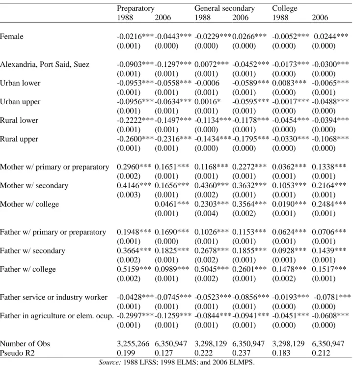
Table 2 presents probit model estimates of the relationship between educational attainment and circumstances beyond the control of an individual in 1988 and 2006. The effects of circumstance variables on completion of preparatory, general secondary and college education are substantial. Other things being equal, girls are less likely to complete basic education over the entire period (with differentials of 2 in 1988 and 1998 and 4 points in 2006). However, gender gaps have decreased at general secondary and college levels. The disadvantage of girls has disappeared over the period and even been reversed at secondary levels with girls 3 percent more likely than boys to complete general secondary education in 2006. Similarly, the disadvantage of girls at higher education levels was reversed with a 2 percent higher completion of college in their favor in 2006.
The differentials between youth of different family backgrounds also tend to decrease over time. For instance, at basic education (preparatory) level, the differential associated with the agricultural (or elementary) occupation of a father (13 points in 2006), as the one associated with parental education, were declined by more than twice. Similarly, although youth born in rural lower and upper Egypt are much less likely to complete basic education (respectively 23 and 15 points less in 2006, compared to youth born in Cairo), the gaps between rural and urban areas have decreased somewhat over the period (although the progress is limited in Upper Egypt). Thus the expansion of enrollment at basic education seems to have benefited youth from disadvantaged
backgrounds and rural areas.
However, the gaps associated with parental background and region of birth have not diminished at upper education levels, where completion rates have increased mostly for kids from more privileged backgrounds. At the general secondary level, youth born in rural Upper Egypt are 14 and 18 percent points less likely to attain a general secondary education in 1988 and 2006, respectively. Youth whose father has an agricultural (or elementary) occupation seem to be at a higher disadvantage in 2006 than in 1988, with 9 percentage points lower likelihood to attain a general secondary degree. And the differentials associated with mother’s education are persistent.
Similarly, at college level, the differentials associated with region and family background persist and have even increased over the entire period. For instance, youth born in rural upper Egypt are 11 percentage points less likely than those born in Great Cairo to attain a college education in 2006 (3 points in 1988). Children of agricultural workers are 6 percentage points (4.5 points in 1988) less likely than children of higher occupation fathers. Youth whose mothers are uneducated are 22 percentage points (11 points in 1988) less likely than those whose mothers have attained secondary education.
In general, while basic education has democratized, barriers to access to general secondary and college education have remained for kids from disadvantage backgrounds. This is a sign of the increased competition taking place for accessing general senior-secondary schools and universities.
Table 2: Circumstances and completion rates: Probit estimates
Preparatory General secondary College
1988 2006 1988 2006 1988 2006 Female -0.0216*** -0.0443*** -0.0229*** 0.0266*** -0.0052*** 0.0244***
(0.001) (0.000) (0.000) (0.000) (0.000) (0.000) Alexandria, Port Said, Suez -0.0903*** -0.1297*** 0.0072*** -0.0452*** -0.0173*** -0.0300***
(0.001) (0.001) (0.001) (0.001) (0.000) (0.000) Urban lower -0.0953*** -0.0558*** -0.0006 -0.0589*** 0.0083*** -0.0065*** (0.001) (0.001) (0.001) (0.001) (0.000) (0.001) Urban upper -0.0956*** -0.0634*** 0.0016* -0.0595*** -0.0017*** -0.0488*** (0.001) (0.001) (0.001) (0.001) (0.000) (0.000) Rural lower -0.2222*** -0.1497*** -0.1134*** -0.1178*** -0.0454*** -0.0394*** (0.001) (0.001) (0.000) (0.001) (0.000) (0.000) Rural upper -0.2600*** -0.2316*** -0.1434*** -0.1795*** -0.0330*** -0.1068*** (0.001) (0.001) (0.000) (0.000) (0.000) (0.000) Mother w/ primary or preparatory 0.2960*** 0.1651*** 0.1168*** 0.2272*** 0.0362*** 0.1338***
(0.002) (0.001) (0.001) (0.001) (0.001) (0.001) Mother w/ secondary 0.4146*** 0.1656*** 0.4360*** 0.3632*** 0.1053*** 0.2164***
(0.003) (0.001) (0.002) (0.001) (0.001) (0.001) Mother w/ college 0.0461*** 0.2303*** 0.3564*** 0.0190*** 0.2484***
(0.001) (0.004) (0.002) (0.001) (0.001) Father w/ primary or preparatory 0.1948*** 0.1690*** 0.1026*** 0.1153*** 0.0624*** 0.0706***
(0.001) (0.000) (0.001) (0.001) (0.001) (0.001) Father w/ secondary 0.3664*** 0.1825*** 0.2678*** 0.1855*** 0.0928*** 0.1439***
(0.002) (0.001) (0.002) (0.001) (0.001) (0.001) Father w/ college 0.5159*** 0.0989*** 0.5045*** 0.2601*** 0.1478*** 0.1517***
(0.002) (0.001) (0.002) (0.001) (0.002) (0.001) Father service or industry worker -0.0428*** -0.0745*** -0.0523*** -0.0856*** -0.0193*** -0.0781***
(0.001) (0.001) (0.001) (0.001) (0.000) (0.000) Father in agriculture or elem. ocup. -0.2997*** -0.1259*** -0.0844*** -0.0941*** -0.0451*** -0.0608***
(0.001) (0.001) (0.001) (0.001) (0.000) (0.000) Number of Obs 3,255,266 6,350,947 3,298,129 6,350,947 3,298,129 6,350,947 Pseudo R2 0.199 0.127 0.222 0.237 0.183 0.212
Source: 1988 LFSS; 1998 ELMS; and 2006 ELMPS.
Sample: 21-24 year-olds; reference categories are: boy, birth in Great Cairo, uneducated mother (or missing value),
uneducated father (or missing value), and father professional, manager, technician or clerck. p<0.10, ** p<0.05, *** p<0.01;
Least and most advantaged groups
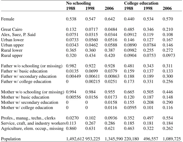
Another way of illustrating the stark disparities among circumstance groups is to compare students belonging to the extremes of the distribution of educational attainments. For this purpose, Table 3 describes the characteristics of the youth who do not complete basic education and of those who attain a college education. Uneducated youth consist in more than 1,300,000 individuals aged
21-24 in 2006 (that number decreased only slightly from 1,500,000 in 1988), and the share of girls increases among them to reach two thirds for that year. They tend to be more concentrated in rural areas (more than 80 percent in 2006), are in great majority children of uneducated parents (more than 90 percent in any year), and children of agricultural (or elementary) workers (more than 60 percent in 2006). At the other end, college graduates vastly increased from about 220,000 individuals aged 21-24 in 1988 to more than 1,100,000 in 2006; girls became the majority of them (57 percent in 2006). While the share of college graduates in rural Lower Egypt increased, no increased observed in rural Upper Egypt. The shares of individuals from more disadvantaged backgrounds diminished among college graduates. For instance the share of children from agricultural or elementary workers diminished from 46 to 26 percent, while the share of children of higher occupation fathers increased from 35 to 55 percent.
Table 3: Characteristics of youth with low and high educational attainment
No schooling College education
1988 1998 2006 1988 1998 2006
Female 0.538 0.547 0.642 0.440 0.534 0.570
Great Cairo 0.132 0.0717 0.0484 0.485 0.346 0.210
Alex, Suez, P. Said 0.0751 0.0315 0.0344 0.0912 0.119 0.108
Urban lower 0.0733 0.0560 0.0516 0.146 0.127 0.167
Urban upper 0.0343 0.0462 0.0588 0.0890 0.0784 0.146
Rural lower 0.365 0.360 0.387 0.0982 0.255 0.272
Rural upper 0.320 0.434 0.420 0.0904 0.0753 0.0973
Father w/o schooling (or missing) 0.982 0.922 0.928 0.481 0.343 0.311 Father w/ basic education 0.0135 0.0699 0.0379 0.159 0.137 0.133 Father w/ secondary education 0.00449 0.00611 0.00863 0.188 0.189 0.300 Father w/ college education 0 0.00215 0.0251 0.173 0.331 0.256 Mother w/o schooling (or missing) 0.994 0.984 0.955 0.665 0.505 0.446 Mother w/ basic education 0.00556 0.0156 0.0173 0.120 0.187 0.148 Mother w/ secondary education 0 0 0.0158 0.155 0.208 0.290 Mother w/ college education 0 0 0.0116 0.0595 0.101 0.116 Profes., manag., techn., clerks 0.0270 0.102 0.0936 0.352 0.497 0.554 Service, craft, and industry workers 0.113 0.267 0.286 0.185 0.181 0.184 Agriculture, elem. occup., missing 0.860 0.631 0.621 0.463 0.322 0.262 Population 1,492,612 953,225 1,345,590 220,180 496,557 1,089,725
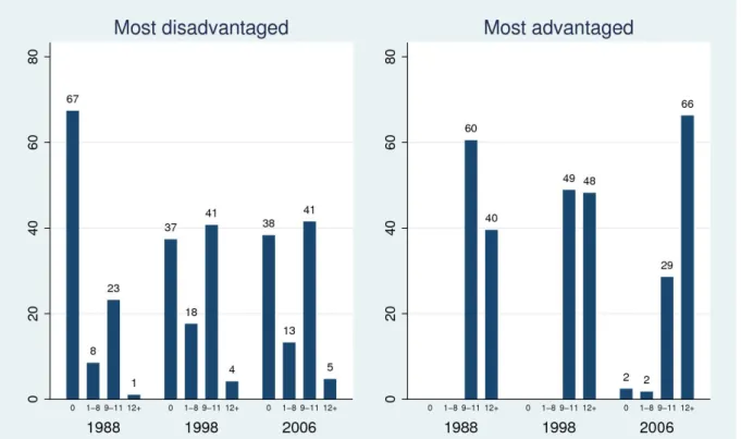
Figure 1 shows the distribution of attainments for 21-24 year-olds for the least and most advantaged groups. Least advantaged youth are defined as those with unfavorable circumstances, such as being born in rural areas, from uneducated parents, and having a father with elementary or subsistence agriculture job. On the other hand, most advantaged youth are defined as those with favorable characteristics, namely being born in urban areas of the Greater Cairo, Alexandria, Suez, or Port Saïd, from parents with secondary or higher education, and having a father with higher occupational status (professional, manager, technician, or clerk). The least advantaged account for 25 percent of the population of 21-24 year-olds in 1998 and 2006 (and slightly more, 27 percent, in 1988), while the most advantaged account for 3 percent of the population in 1998 and 2006 (and 2 percent in 1988). As expected, the prospects of the two groups are strikingly different: in 2006, only 5 percent of the least advantaged have attained a college education, 41 percent a secondary one, 13 percent a primary one, and 38 percent never attended school. On the contrary, 65 percent of the most advantaged have attained a college education, 29 percent secondary, and only 4 percent did not complete secondary education. There is evidence of democratization between 1988 and 1998: the share of never attenders decreased substantially from 67 to 37 percent among the least advantaged and many of them were able to accessed basic education. However, progress in equity seems to have halted in the 2000s. The share of college graduates increased by 17 points among most advantaged, while there was no appreciable increase among the least advantaged.
Figure 1: Attainments among least and most advantaged groups
Note: Distribution of most disadvantaged and most advantaged youth (above defined) by educational attainment in 1988, 1998, and 2006. Source: ELMPS surveys. Sample: 15-19 year-olds.
Drop-out rate
A similar picture emerges when looking at drop-out rate among those who participated in the 2007 TIMSS survey of 8th graders. Consider 15-19 year-olds in 2006, most out-of-school
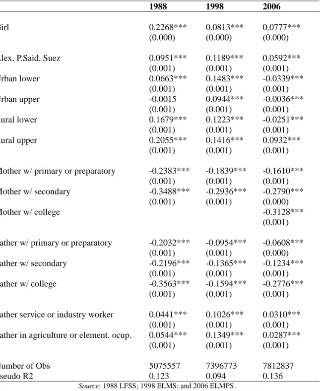
children actually never enrolled (about 13 percent of 15-19 year-olds in 2006) or dropped out after obtaining some vocational secondary education (15 percent). Drop-outs after primary (7 percent) or preparatory (4 percent) are less frequent. Table 4 reports results from a partial correlations analysis of drop-out, i.e. probit estimates of the marginal effects of a set of circumstance variables for the same samples of 15-19 year-olds in 1988 and 2006. Girls have more often dropped out than boys, but the gap decreased from 23 to 8 points between 1988 and 2006. While large geographic differentials persist in drop-out rate, there are continuous improvements over the last two decades. Children born in rural Upper Egypt continue more likely to drop out than those born in any other
region but the gap decreased from 21 to 9 points, compared to Greater Cairo. However some gaps associated with family background have only slightly diminished, e.g. children with uneducated parents are still much more likely to have dropped-out in 2006 (about 30 points more than children of college graduates).
Table 4: Circumstances and drop-out rate: Probit estimates
1988 1998 2006
Girl 0.2268*** 0.0813*** 0.0777***
(0.000) (0.000) (0.000)
Alex, P.Said, Suez 0.0951*** 0.1189*** 0.0592***
(0.001) (0.001) (0.001) Urban lower 0.0663*** 0.1483*** -0.0339*** (0.001) (0.001) (0.001) Urban upper -0.0015 0.0944*** -0.0036*** (0.001) (0.001) (0.001) Rural lower 0.1679*** 0.1223*** -0.0251*** (0.001) (0.001) (0.001) Rural upper 0.2055*** 0.1416*** 0.0932*** (0.001) (0.001) (0.001) Mother w/ primary or preparatory -0.2383*** -0.1839*** -0.1610***
(0.001) (0.001) (0.001)
Mother w/ secondary -0.3488*** -0.2936*** -0.2790***
(0.001) (0.001) (0.000)
Mother w/ college -0.3128***
(0.001) Father w/ primary or preparatory -0.2032*** -0.0954*** -0.0608***
(0.001) (0.001) (0.000)
Father w/ secondary -0.2196*** -0.1365*** -0.1234***
(0.001) (0.001) (0.001)
Father w/ college -0.3563*** -0.1594*** -0.2776***
(0.001) (0.001) (0.001) Father service or industry worker 0.0441*** 0.1026*** 0.0310***
(0.001) (0.001) (0.001) Father in agriculture or element. ocup. 0.0544*** 0.1349*** 0.0287***
(0.001) (0.001) (0.001)
Number of Obs 5075557 7396773 7812837
Pseudo R2 0.123 0.094 0.136
Source: 1988 LFSS; 1998 ELMS; and 2006 ELMPS. Note: * p<0.10, ** p<0.05, *** p<0.01.
Sample: 15-19 year-olds; reference categories are: boy, birth in Great Cairo, uneducated mother (or missing value),
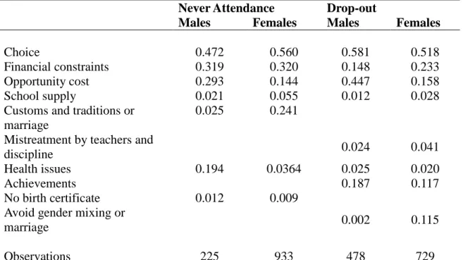
Table 5 document the reasons reported for never attending school and dropping out (using information collected among 10-29 year-olds by the SYPE 2009 survey). About half of never-attenders report family or own choice as a reason for not going to school. A higher proportion for girls reported that cultural views toward gender roles still enter in these decisions. Financial constraints and opportunity costs of schooling (i.e. the foregone economic contribution of children attending school) were mentioned by 52 and 46 percent of never-attending boys and girls, respectively. Customs, traditions and marriage are cited as reasons by 24 percent of girls. Hence, when availability of schools is not a prominent reason, lack of financial resources and cultural attitudes toward girls’ schooling are the main reasons reported for never attendance. Similarly, financial constraints and opportunity costs are cited for dropping-out by 60 and 39 percent of boys and girls, respectively. Avoiding mixing with opposite gender or marriage was cited for 11 percent of girls for dropping-out.
Table 5: Reasons for never attending and dropping out of school Never Attendance Drop-out
Males Females Males Females
Choice 0.472 0.560 0.581 0.518
Financial constraints 0.319 0.320 0.148 0.233
Opportunity cost 0.293 0.144 0.447 0.158
School supply 0.021 0.055 0.012 0.028
Customs and traditions or marriage
0.025 0.241
Mistreatment by teachers and
discipline 0.024 0.041
Health issues 0.194 0.0364 0.025 0.020
Achievements 0.187 0.117
No birth certificate 0.012 0.009
Avoid gender mixing or
marriage 0.002 0.115
Observations 225 933 478 729
3.
Inequities in learning achievements
In section 2, we showed that while there has been democratization in access to basic education, there remain persistent disparities in access to general secondary and college education. Given that educational trajectories depend to a large extent on the early tracking into general and vocational secondary schools at completion of basic education, the quality of the education at lower levels of schooling is likely to be a major determinant of educational inequalities in Egypt.4 We now
turn to inequalities in learning achievements, as measured by TIMSS pupils’ achievements evaluation, at the end of basic education. For investigating learning achievements at completion of basic education, we use information from the Trends in International Mathematics and Science Studies conducted in Egypt in 2003 and 2007. These surveys collected responses, from a representative sample of Egyptian eight-graders, to series of items of a test-based evaluation of achievements in Math and Science. 7,095 pupils of 217 schools were interviewed in 2003 and 6,582 pupils in 233 schools in 2007.5
Achievements in Math and Science are measured using item response theory models, aggregating answers from many test items of varying difficulty and discriminating power. Those models treat achievement as a latent variable, and, assuming a given distribution (usually a normal) for the achievements of pupils, their estimation allows deriving its distribution and its predicted value for each individual (see Mislevy, 1991; Mislevy et al., 1992). Importantly, these models recover estimates of individual achievements that come with a scale that is arbitrarily fixed. Essentially, there is no scale for measuring a pupil’s scholastic ability, so that some reference levels have to be fixed for the mean and standard deviation of achievement measured by a test. International achievement tests thus fix those reference levels of mean and standard deviation for a given set of country and year, and the subsequent evaluations conducted with the same test are reported using the same arbitrary scale. In the TIMSS procedure, test-scores were normalized by
4 The tracking is determined by scores at the preparatory completion exam organized at the level of governorates. 5 We report the results for Math test-scores. The results for Science are very similar and available upon request.
fixing the mean and standard deviation of achievements of pupils who participated to the first 1995 international TIMSS survey at respectively 500 and 100. This standardization must be dealt with in inequality measurement.
The TIMSS surveys collected information on children’s background, in particular, in addition to their gender, mother’s and father’s education, the language spoken at home, whether any of the parents was born abroad, household ownership of durables such as books, tv sets, satellite channels access systems, and phones. The information on the economic status of the parents is limited though, with parental, notably father’s, educational attainments serving as an imperfect proxy. Besides, the surveys indicate the location of the schools, which we take as a proxy for places where children were raised.6 For the 2007 survey, we could use information on the governorate and area
type (urban or rural) of the school location. For the 2003 survey, we could only access the area type information.7
Methodology for measuring learning opportunity inequality
The inequality measures to be used for documenting the distributions of test scores must account for several methodological issues. In particular they must be robust to the standardization of those variables. However, as noted by Ferreira and Gignoux (2011a), no inequality index satisfying a set of basic desirable properties (symmetry, continuity and the transfer principle) can be both scale- and translation invariant, and thus robust to the standardization. A number of well-known inequality indices, such as the Gini and Generalized Entropy indexes, are not even ordinally equivalent, so that the arbitrary standardization could affect the ranking of different population by inequality levels.
For handling this standardization issue, we follow Ferreira and Gignoux (2011a), and base
6
Migrations motivated by studies should be limited among 8 graders. The SYPE survey provides no information on birth place of children less than 15.
7The definition of urban areas is not perfectly consistent across the 2003 and 2007 surveys. The 2003 information relies
on a classification of “communities” by population size (communities with more than 50,000 inhabitants are classified
as urban), while the 2007 information is the official classification consists in the administrative classification (which was not available in 2003).
our inequality analysis on the variance (and standard deviation). Consider a post-standardized distribution of test-scores (yi), obtained as a linear function of the pre-standardization distribution
(xi), where � denotes a student:
= �̂ +�̂� − � (1)
The variance (or standard deviation) of a post-standardized distribution (Vy), for example, is a monotonic (proportional) function of the pre-standardization variance (Vx), and does not depend on any other moment of the pre-standardization distribution; for the variance:
� = �̂� � (2)
While it is not scale invariant, the mean (as the standard deviation) is thus ordinally-invariant to the standardization. In addition it satisfies the basic properties abovthe e (and is also additively decomposable). It thus provides a basic standardization ordinally consistent measure of inequality of educational achievement. In practice, we report the standard deviation.
In this paper, rather than overall inequality, we are mainly interested in inequality of achievement opportunity. Following Roemer (1998), empirical analyses of the distribution of opportunities begin by seeking agreement on a set of individual characteristics which are beyond the individual’s control, and for which he or she cannot be held responsible. These variables are called ‘circumstances’. Once a vector C of circumstances has been agreed upon, the population can be partitioned into groups with identical circumstances. Such a partition can be denoted Π = {� , � , … , ��}, where each � = 1, … , � is a set of specific values taken by the circumstance
variables (a circumstance group or ‘type’ in Roemer’s terminology).
In one approach to the measurement of inequality of opportunity, called ex-ante and associated with van de Gaer (1993), the opportunity set faced by each type is evaluated using the conditional distributions of outcomes given circumstances, and equality of opportunity is attained when there is perfect equality in those values across all types. This rests on the notion that purely individual effort or ability should be orthogonal to an individual’s circumstances at birth (for more
discussion, see e.g. Roemer, 1998; Fleurbaey, 2008).8 The full conditional distributions of outcomes
given types or some of its higher moments can be used, but, in practice, researchers have often used the mean income (or achievement) of the type as an estimate of the value of the opportunity set they face. Since equality of opportunity would imply equality in means across types, inequality of opportunity is then naturally seen as some measure of between-type inequality. As in Ferreira and Gignoux (2011a, b), we thus measure inequality of opportunity (IOp) by between-type inequality, or specifically:
��� =
� {���}
� (3)
where {� } is the smoothed distribution corresponding to the distribution y and the partition P.
Following Bourguignon et al. (2007) and Ferreira and Gignoux (2011b), one can obtain a parametric estimate for ���, based on an OLS regression of y on C:
̂��� = �(��′�̂)
� (4)
�̂ in (4) is the OLS estimate of the regression coefficients in a simple regression of y on C:
� = �′� + � (5)
In (4), the denominator is an inequality measure computed over the vector of predicted incomes from regression (5). Under the maintained assumption of a linear relationship between achievement and circumstances, this vector is equivalent to the smoothed distribution, since all individuals with identical circumstances are assigned their conditional mean incomes.
Following the arguments above, we use the simple variance as our inequality index I( ). This choice yields our proposed measure of inequality of educational opportunity, as a special case of
8In an alternative but closely related approach, called ex-post and associated with Roemer (1998), equality of
opportunity obtains only when individuals exerting the same degree of effort, regardless of their circumstances, receive the same reward. See Fleurbaey and Peragine (forthcoming) for a formal discussion of the relationship between the two approaches.
(4):
̂��� = ��� (��′�̂)
��� � (6)
This is the R-squared of an OLS regression of the child’s test score on a vector C of individual circumstances. Despite its simplicity, it is a meaningful summary statistic. It is a parametric approximation to the lower bound on the share of overall inequality in educational achievement that is causally explained by the joint effect of all circumstances. A formal proof is provided by Ferreira and Gignoux (2011b). But the basic intuition is that some circumstances remain unobserved, and observing and controlling for those unobservables could only increase the share of explained inequalities. However, the estimates should not be interpreted as capturing the effects of the specific set of circumstances considered in the analysis as they may reflect the effects of omitted and correlated individual and environmental characteristics. Individual elements of the vector thus suffer from these omitted variable biases, and cannot be interpreted as causal estimates of the individual impact of a particular circumstance on test scores.
Another attractive feature of ̂��� as a measure of inequality of educational opportunity is that, unlike any measure of the level of inequality, it is a parametric estimator of a ratio (equation (3)) that is cardinally invariant in the standardization of test scores. To see this, note that any sub-group mean is affected by standardization in a manner analogous to equation (1), so that:
��� {� } = �̂� ��� {� } (7)
Given (7) and equation (2), it follows that: ��� =��� {��
� }
��� =
��� {��� } ���
Finally, ̂��� is decomposable into components for each individual variable in the vector C. Equation (6) can be rewritten as the sum over all elements (denoted by j) of the C vector:9
9This is an example of a Shapley-Shorrocks decomposition: it corresponds to the average between two alternative paths
for estimating the contribution of a particular circumstance CJ to the overall variance. In the first (direct) path, all Cj, j ≠
J are held constant. In the second (residual) path, Cj is itself held constant, and its contribution is taken as the difference
between the total variance and the ensuing variance. Either path is conceptually valid, and the Shapley-Shorrocks averaging procedure yields (8) as the path-independent additive decomposition. See Shorrocks (1999) for the original
̂��� = ∑ ̂ = ∑ ��� − [� ��� � + ∑ � � ��� (� , � )] (8)
Beyond the specific measures to be used, an additional challenge is that the TIMSS sample is representative of eighth-graders and not of the overall population of lower-secondary school age children. An estimate of the share preparatory-level graduates among those cohorts can be obtained from the SYPE survey: 78 percent of youth between 16 and 21 complete preparatory schooling. Thus 22 percent drop out before and their achievements are not reflected in a basic analysis of TIMSS test-scores.10 This selection is problematic for an analysis of educational opportunities
which is not concerned only in the outcomes of preparatory-level enrollees. Dropping out is extremely likely to be a selective process, in the sense that it is correlated with family and student characteristics that also affect test scores. Correcting for the selection biases is thus not simple.
The approach here follows Ferreira and Gignoux (2011a), and consists of a simple two-sample non-parametric mechanism for assessing the sensitivity of our inequality measures to alternative assumptions about the sample selection process. The procedure relies on using information on preparatory school graduates from the HIECS Egyptian budget survey from 2004-05. This large-sample survey allows estimating the numbers of preparatory-school graduates and drop-outs in groups defined by similar gender, father’s education and region of residence (the two later variables have consistent coding in the two surveys). The procedure then consists in putting back observations and imputing test-scores for drop-outs in the TIMSS sample. Two extreme assumptions are used for the imputations. The first assumes selection on observables whereby drop-outs would achieve similarly to children taking the TIMSS tests that have similar characteristics. The second assumes selection on both observables and (strongly) unobservables and attributes a test-score in the lower tail (we use the 5th quintile) of the conditional distribution of scores achieved by test takers with similar characteristics. In practice, the corrections are implemented by a
application of the Shapley value to distributional decompositions. Ferreira and Gignoux (2011a) provide a formal proof that (8) is the Shapley-Shorrocks decomposition of the variance into the effects of individual circumstances.
10
Among those, 6.5 percent have never been to school, 4.5 dropped out before completing primary, and 11 percent before completing preparatory.
weighting of the TIMSS sample.
Learning achievement inequality: low mean and high dispersions
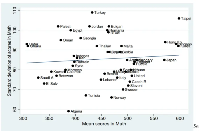
For applying the measures above to the TIMSS data, we first document the levels of inequality in learning achievement observed in Egypt and put them in an international perspective. Figure 2 plots the country-level standard deviations of test scores against the mean scores in Math in the TIMSS 2007 data. Egypt, with a mean score of 391 and a standard deviation of 100, lies in the top left quadrant, i.e. has both a low mean and a high dispersion in learning achievements. Jordan, Oman and Palestine have similar means and inequality levels, but Egypt has one of the highest inequality levels (Turkey has an even more dispersed distribution of achievements but with a higher mean). The main implication of this pattern is that, although it also has high performers, Egypt has a large number of pupils performing very low at the TIMSS test. We then document the gender gaps.
Figure 2: Mean and inequality in Math test-scores: Egypt in an international comparison
Sour ce: 2007 TIMSS student achievement surveys.
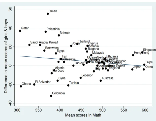
country mean. In average, girls score 13 points above boys in Math in Egypt (397 against 384). This moderate differential in favor of girls contrasts with their lower access rates at basic education levels. A similar higher mean performance of girls is observed (and sometimes larger) in other MENA countries (Bahrain, Jordan, Palestine, Oman, Qatar, Saudi Arabia), but boys still perform better than girls in others (Algeria, Lebanon, Morocco, Syria, Tunisia), so that Egypt does not stand apart on this gender differential, and gender-based inequalities are not driving the large level of learning inequality observed in Figure 2. We then document the gender gaps.
Figure 3: Gender-differential and mean Math test-scores: Egypt in an international comparison
Source: 2007 TIMSS student achievement surveys.
A high absolute level of inequality of learning opportunity
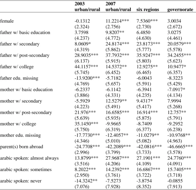
Now let us turn to inequality in learning opportunities. OLS estimates of the partial effects of circumstances on achievements in Math are reported in Table 6. For TIMSS 2007, we report the estimates with three different sets of geographic controls, for a) urban and rural governorates, b) six regions, and c) all governorates. When the more detailed geographic controls are used, gender has
effects on scores neither in 2003 nor in 2007. Parental education does have large effects on test-scores with gaps of about 30 points between children of post-secondary graduates and those of uneducated parents. Other things equal, children of parents born abroad achieve lower (by 25 to 45 points) test-scores, and there are also some differentials associated with spoken language although those speaking Arabic and another language now perform better (by 10-25 points). Ownership of a tv set, probably capturing some wealth effects, is associated with a large differential (of 20-45 points) (ownership of a phone also matters), while ownership of books with smaller (about 10 points) ones (cultural resources are probably already captured by parental education). Differentials associated with location are also large with children in rural performing in average 40 points below in 2007 and those of rural Upper Egypt almost 75 points below those in urban Lower Egypt.
Table 6: OLS Regressions of Standardized Math Test Scores on Circumstances
2003 2007
urban/rural urban/rural six regions governorate female -0.1312 11.2214*** 7.5360*** 3.0034
(2.324) (2.756) (2.730) (2.672) father w/ basic education 3.7598 9.8207** 6.4850 3.0275 (4.237) (4.772) (4.630) (4.461) father w/ secondary 8.0609* 24.8174*** 23.8173*** 20.0579*** (4.319) (5.862) (5.777) (5.578) father w/ post-secondary 28.9035*** 37.7932*** 35.9247*** 34.2455*** (6.137) (5.915) (5.803) (5.623) father w/ college 44.1157*** 14.5372** 12.9275** 10.9477* (5.745) (6.452) (6.465) (6.357) father edu. missing -13.9200*** -5.7182 -6.0043 -8.3223
(4.769) (5.657) (5.591) (5.429) mother w/ basic education -6.2337 -6.1142 -6.3941 -7.0917*
(3.886) (4.331) (4.235) (4.134) mother w/ secondary -5.5929 12.5279** 9.4317* 7.9994 (4.223) (5.491) (5.417) (5.268) mother w/ post-secondary 21.976*** 16.6585*** 16.914*** 12.757** (5.639) (5.935) (5.875) (5.791) mother w/ college 35.1450*** -9.9665 -8.7409 -9.2952 (5.750) (6.319) (6.377) (6.238) mother edu. missing -17.7730*** -12.4057** -11.0279** -10.9768**
(4.346) (5.010) (5.082) (4.963) parent(s) born abroad -24.7708*** -42.2089*** -42.0816*** -46.6665***
(2.996) (3.799) (3.733) (3.578) arabic spoken: almost always 13.8799*** 27.9687*** 27.1901*** 24.7760***
(3.516) (4.206) (4.109) (4.091) arabic spoken: sometimes 8.2022*** 14.2392*** 16.6867*** 15.7405***
(2.950) (3.761) (3.722) (3.718) arabic spoken: never -14.3242** -7.5273 -3.8754 -0.0855
books at home: 11-25 -1.1348 -3.0248 -1.3487 -0.5250 (2.791) (3.384) (3.313) (3.218) books at home: 26-100 9.0014** 6.3848 9.0688** 9.0645** (3.746) (4.045) (3.967) (3.921) books at home: >100 4.9763 1.4673 6.3031 7.1206 (4.466) (5.062) (5.006) (4.917) tv owned 45.9552*** 26.5948*** 22.6609*** 24.5407*** (4.640) (5.245) (5.167) (5.069) satelite owned -13.6241*** 6.0568** 7.9091*** 6.9546** (2.395) (2.950) (2.896) (2.825) telephone owned 6.7064** 10.2867*** 9.2801** 8.9792** (2.726) (3.816) (3.729) (3.677) urban area 14.2031*** 35.3493*** 37.8641*** (2.424) (2.949) (3.549) Alx, Sz, Said 3.6656 (4.929) Urban lower 19.0216*** (4.933) Urban upper -4.9274 (4.878) Rural lower -7.0962 (4.353) Rural upper -55.3107*** (4.378) Governorates No No No Yes Constant 350.1*** 325.2*** 358. 7*** 269.9*** (5.502) (6.256) (7.098) (13.278) Number of Obs 7095 6582 6582 6582 R-squared 0.210 0.181 0.210 0.239
Source: TIMSS 2003 and 2007 surveys.
Sample: TIMSS 2003 and 2007 samples of eight-graders.
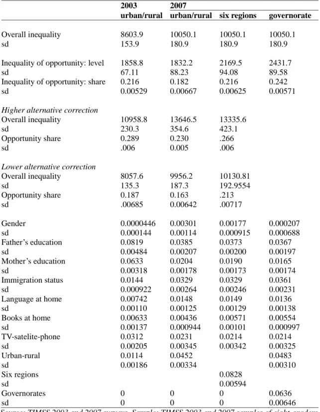
The estimates of the opportunity shares of inequalities in achievements at the TIMSS Math test are shown in Table 7. The results for 2007 (column 2) with a similar urban-rural specification to the 2003 results give a lower bound for the opportunity share at 18.2 without the imputations. It is lower than the 2003 one by 3.4 percent; the decrease has a standard error of .85 point, so it is statistically significant at usual levels. When accounting for drop-outs,the ranges obtained with the imputations for 2003 and 2007 overlap, which makes it difficult to conclude on the changes in equity in learning achievement between 2003 and 2007. The two remaining columns use more detailed information on geography from the 2007 data. The lower bound increases to 21.6 percent with the six regions school location variable (and vary between .213 and .266 with the imputations) and to 24.2 percent when accounting for the precise governorates for school locations. This increase
suggests that achievement inequalities associated with geography are large. Overall, based on the last more complete estimates, at least a quarter of achievement inequalities at the end of preparatory can be attributed to circumstances. This estimate is average in an international perspective (the share of inequality of opportunity was found similar in countries such as UK or the US in Ferreira and Gignoux, 2012), but, given the high overall learning inequalities, the absolute level of learning inequities at completion of basic education is higher in Egypt than in many other countries.
The estimates of partial shares associated with specific circumstances confirm the importance of geography. Using data on Math test-scores in 2007, 4.5 percent of inequalities are accounted for by area type in the first model, 8.3 percent by the six regions indicators in the second, and 11.2 percent by area type and governorate together in the third. In comparison, the next most important circumstances are parental education (3 to 4 percent for father’s and about 2 percent for mother’s education), and immigration status (3 to 4 percent), and ownership of cultural goods which accounts for another 3 percent. Language at home accounts for about 1.5 percent. Gender is not associated with a significant share of inequalities in achievements.
Table 7: Opportunity Share of Inequality in Educational Achievement
2003 2007
urban/rural urban/rural six regions governorate Overall inequality 8603.9 10050.1 10050.1 10050.1
sd 153.9 180.9 180.9 180.9
Inequality of opportunity: level 1858.8 1832.2 2169.5 2431.7
sd 67.11 88.23 94.08 89.58
Inequality of opportunity: share 0.216 0.182 0.216 0.242 sd 0.00529 0.00667 0.00625 0.00571
Higher alternative correction
Overall inequality 10958.8 13646.5 13335.6
sd 230.3 354.6 423.1
Opportunity share 0.289 0.230 .266
sd .006 0.005 .006
Lower alternative correction
Overall inequality 8057.6 9956.2 10130.81 sd 135.3 187.3 192.9554 Opportunity share 0.187 0.163 .213 sd .00685 0.00642 .00717 Gender 0.0000446 0.00301 0.00177 0.000207 sd 0.000144 0.00114 0.000915 0.000688 Father’s education 0.0819 0.0385 0.0373 0.0367 sd 0.00484 0.00207 0.00200 0.00197 Mother’s education 0.0633 0.0204 0.0190 0.0165 sd 0.00318 0.00178 0.00173 0.00174 Immigration status 0.0144 0.0329 0.0329 0.0361 sd 0.000922 0.00264 0.00246 0.00231 Language at home 0.00742 0.0148 0.0149 0.0136 sd 0.00110 0.00125 0.00129 0.00138 Books at home 0.00633 0.00436 0.00571 0.00554 sd 0.00137 0.000944 0.00101 0.000997 TV-satelite-phone 0.0312 0.0231 0.0214 0.0214 sd 0.00205 0.00345 0.00342 0.00325 Urban-rural 0.0114 0.0452 0.0483 sd 0.00186 0.00334 0.00310 Six regions 0.0828 sd 0.00594 Governorates 0 0 0 0.0636 sd 0 0 0 0.00646
Source: TIMSS 2003 and 2007 surveys. Sample: TIMSS 2003 and 2007 samples of eight-graders.
Significant achievement inequality in national exams
To investigate how learning opportunities evolve across schooling levels, here we expand the analysis to achievements at national exams at primary, preparatory, and secondary levels. We use retrospective data from the Survey of Young People of Egypt in 2009 (Asia and Office, 2011).
The survey collected detailed information from a sample of 15,029 individuals aged 10 to 21. Notably, it asked information on whether individuals completed different schooling levels, and their scores in the national examinations at completion of the primary, preparatory, and secondary levels. Examination scores take values ranging between 50 and 100. The average score is 82.0 (with standard deviation of 11.5) at the primary, 75.2 (13.2) at the preparatory, and 74.9 (12.8) at secondary levels.11 We focus on scores of 12-15 year-olds at primary, 14-18 year-olds at the
preparatory, and 18-21 year-olds at the secondary completion. Among individuals of those age groups who completed those attainments, respectively 59, 72 and 82 percent reported exam scores.
The 2009 SYPE survey also collected information on the background of the youth. In the analysis below, the set of variables used to capture their background include gender, governorate of birth, parental education level, religion (Muslim vs another religion), and family wealth, obtained from information on the durables owned by households and housing conditions, and their wealth group (i.e., consumption quintiles).12
We perform the analysis of inequality in exam scores using the same approach as for learning achievements evaluated using TIMSS data above. Table 8 reports OLS estimates of the partial effects of circumstances on exam scores. Girls tend to do better at all three exams with a gap of 2 to 4 more exam points on average, increasing with attainment, than boys. The gaps associated with parental education levels are large, ranging from 6 points for father’s education at the primary completion exam to 10 points for mother’s education at the preparatory.13
The gaps associated with family wealth are large—about 8 points at the primary and preparatory completion exams. There are no apparent differentials in scores between Muslims and non-Muslims. However, there are large differentials associated with birth place, with scores for some birth-governorates 13-14 points
11
In an alternative but closely related approach, called ex-post and associated with Roemer (1998), equality of opportunity obtains only when individuals exerting the same degree of effort, regardless of their circumstances, receive the same reward. See Fleurbaey and Peragine (forthcoming) for a formal discussion of the relationship between the two approaches.
12Parental education is not observed, and we recode those variables using a missing value category, for youth who do
not live with their parents.
13Note that the information on parental education is missing for children who do not live with their parents. For those
higher than others at the primary and preparatory completion levels (estimates not reported, available upon request).14
Table 8: OLS Regressions of national Exam Scores and Circumstances
Primary Preparatory Secondary 12-15 y.o. 14-18 y.o. 17-21 y.o. Female 2.1457*** 2.3074*** 3.7964***
(0.594) (0.665) (0.548) Father’s education: primary 1.9986* 1.3525 0.0715 (1.186) (1.191) (1.005) Father’s education: Preparatory/Secondary 3.0621** 0.0195 0.7825 (1.416) (1.440) (1.173) Father’s education: Vocational 4.3131*** 3.0546** -0.2084
(1.229) (1.326) (1.154) Father’s education: Post-secondary 6.3862*** 3.7641** 3.0193**
(1.282) (1.469) (1.277) Father’s education: missing 4.2317*** 1.5136 0.6747 (1.293) (1.257) (1.062) Mother’s education: primary 1.1897 -0.0117 -0.8078
(1.118) (1.142) (0.812) Mother’s education: Preparatory/Secondary 0.2962 2.5697** 0.6547 (1.247) (1.159) (1.166) Mother’s education: Vocational 2.3152** 5.9249*** 3.6505***
(1.064) (1.146) (1.031) Mother’s education: Post-secondary 4.6120*** 9.8281*** 8.0822***
(1.254) (1.318) (1.273) Mother’s education: missing -2.6107* 0.9920 -0.8473
(1.485) (1.648) (1.134) Wealth quintile: second 2.0688* -0.5497 1.2235 (1.212) (1.396) (1.051) Wealth quintile: middle 3.2326*** 0.1682 2.3500**
(1.148) (1.329) (1.016) Wealth quintile: fourth 4.9018*** 2.4809* 3.2626***
(1.204) (1.358) (1.055) Wealth quintile: highest 7.7830*** 6.5910*** 5.5169***
(1.260) (1.514) (1.249) Religion: Non-Muslim -0.3049 -0.3096 0.5954 (1.568) (1.681) (1.052) Birth Governorates Yes Yes Yes Constant 72.9671*** 71.7394*** 62.3858***
(1.829) (2.999) (2.580)
Number of Obs 1497 1525 1718
R-squared 0.244 0.306 0.224
Source: SYPE 2009 survey.
Sample: 12-14 y.o. primary, 14-18 y.o. preparatory, and 17-21 y.o. secondary graduates. * p<0.10, **p<0.05,*** p<0.01
14
Interestingly, the gaps by birth place are lower at the secondary level, suggesting that the pupils who attain that level are already quite selected.
The estimates of opportunity shares in the distribution of exam scores are shown in Table 9. For scores at the primary completion exam, the set of circumstances used explains 24.4 percent of the overall variation in scores. This estimate varies very little with the lower alternative correction for selection, and increases to 29.1 percent with the upper-bound alternative. For scores at the preparatory completion, the uncorrected estimate is at 30.2 percent, and varies between 27.4 and 35.2 with the correction for selection. Finally, for scores at the secondary completion, the uncorrected estimate is at 22.4 percent, and varies between 20.8 and 27.9 percent with the corrections.
The pattern of increasing and, later on, decreasing shares of inequality explained by circumstances may be only apparent and driven by selection, as the latter is likely to be larger at the secondary level, while the majority of pupils do complete preparatory. But the main result here is that learning opportunity inequality appears at early ages: a large amount of it (at least a quarter of achievement inequality) is already observed at the primary level. Those inequities then build up to reach at least a third of learning inequality at the end of preparatory. Hence, tracking at the end of preparatory does not seem to explain all subsequent inequalities.
Table 9: Opportunity Share of Inequality in National Exam Scores
Primary Preparatory Secondary 12-15 y.o. 14-18 y.o. 17-21 y.o. Overall inequality 134.0 180.0 131.4 Inequality of opportunity: level 32.70 55.05 29.45 Inequality of opportunity: share 0.244 0.306 0.224 Overall inequality - lower correction 137.8 182.1 121.4 Inequality of opportunity: share - lower correction 0.238 0.274 0.208 Overall inequality - upper correction q5 218.3 194.2 156.7 Inequality of opportunity: share - upper correction q5 0.291 0.352 0.279
Gender 0.00769 0.00809 0.0266 Father’s education 0.0633 0.0387 0.0286 Mother’s education 0.0563 0.117 0.0909 Wealth 0.0785 0.0851 0.0510 Religion -0.000044 0.000013 0.00038 Birth governorate 0.0383 0.0574 0.0267 Total sample 1497 1525 1718
Non-missing score sample 2543 2118 2096 Share of non-missing scores 0.589 0.720 0.820 Sample after correction 3246 3975 3719
Source: SYPE 2009 survey.
Sample: 12-14 y.o. primary, 14-18 y.o. preparatory, and 17-21 y.o. secondary graduates.
We also perform the decomposition of the partial shares of scores inequality associated with the different circumstance variables. Birth governorates explain again significant shares of exam scores inequality, notably 6 percent at the preparatory, which seems rather consistent with the result obtained using TIMSS test scores. Family background explains the largest shares of exam scores variations. Parents educational attainments in particular explains respectively 12, 16 and 12 percent of the variation of scores at primary, preparatory, and secondary levels, while family wealth explains 8, 9 and 5 percent of those. Gender explains a significant share of scores inequality only at the secondary exam (3 percent). Again religion has no explaining power. Those results thus suggest that family resources and geography explain most of the variation in achievements at official exams.
4.
Some Evidence on the Determinants of Learning Outcome Inequalities
The findings of section 4 show that a significant share of achievement inequality - at least a quarter or a third depending on whether one considers TIMSS test-scores or preparatory exams - is associated with circumstances determined at birth. They also suggest that those inequities do not appear suddenly at adolescence, notably after the tracking taking place at the end of basic education, but rather build progressively through primary and lower secondary schooling grades.To begin and discuss some factors of educational inequities, Figure 4, based on data from the UNESCO Institute of Statistics, reports the evolution of public spending on education in Egypt, in share of GDP, and benchmarks it with the corresponding public spending in lower middle countries, Arab and Middle East and North Africa countries (note that the series of data are incomplete). It shows that public spending in education has stagnated over the long run (and decreased compared to the early 1980s) and slightly diminished in Egypt over a more recent period between 2003 and 2008, from about 5 to 3.9% of GDP. A similar evolution is observed in other MENA countries but the level of these expenditures is slightly lower in Egypt. The decline in public expenditure on education might contribute to the low learning achievement of many young Egyptians on the TIMSS test.
We now provide a descriptive preliminary analysis of two mechanisms that are likely to contribute to the building of such early learning inequities. We first focus on the choice of attendance of schools of different systems, including public, private (including religious) schools, some of which use English or other languages for teaching, and then consider the effects of the substantial levels of private expenditures in tutoring.
Given the importance of tracking at completion of the preparatory level in the Egyptian education system, those factors may help pupils from specific groups to reach higher achievements at the end of basic education and contribute to diverging educational trajectories at upper levels.
For the analyses below, we use information from the SYPE survey on the type of the primary, preparatory and secondary schools attended by teenagers, distinguishing private, public, but also
experimental language and traditional schools, and on households’ expenditures in private tutoring at the same levels.
Different schools systems
Several school systems coexist in Egypt. The majority of schools depends on the government and teaches in Arabic, but some government experimental schools use English and other languages in addition to Arabic. Besides, many pupils attend private schools; among those, one can distinguish ordinary private schools, language schools that use English for teaching, and religiously-oriented (mainly Al-Azhar, but also Christian) schools. Schools of different systems are managed in diverse ways; for instance private schools, but also experimental government schools, have a more decentralized administration. They also provide different levels of inputs (e.g. teachers and their qualification, infrastructures, or school materials). The attendance of a specific school will also modify the network of school peers with whom a child will interact. The choice of a school system may thus have large effects on learning outcomes, and is likely to be an important channel shaping learning inequities.15
15The levels of inputs and peers networks are also likely to differ across schools within a given system, so the analysis below is far from capturing all the variations in schooling conditions (see the discussion of the results for a specification with schools fixed effects below).
Figure 4: Public spending on education, in percent of GDP
Notes: public spending on education, in share of GDP, in Egypt, lower middle countries, Arab and Middle East and North Africa countries. Source: UNESCO Institute of Statistics (the series
of data are incomplete).
Figure 5 shows the allocation of pupils of different family backgrounds into schools of different systems respectively at the primary, preparatory and secondary levels. We consider a single family background variable here: household wealth.
At the primary level, the great majority of pupils - about 90 percent for each of the first four wealth quintiles - attend government schools, and about 5 percent of pupils of any wealth quintile attend Al-Azhar traditional schools. However, pupils from the highest wealth quintile stand apart, as 35 percent of those attend private or experimental primary schools. A similar pattern emerges at the preparatory level, with most pupils of the first four quintiles attending government schools, or traditional Al-Azhar for a minority, but 25 percent of pupils from the highest quintile attending
3
3,5
4
4,5
5
5,5
6
Egypt, Arab Rep. Lower middle income Arab World
private or experimental schools.
As observed in previous studies, at the secondary level, after tracking into general and vocational schools, children from different family background appear to be allocated into very different systems. Less than 20 percent of pupils from the bottom two quintiles attend general public or private secondary schools, and 75 percent of them attend vocational public schools. At the opposite, 75 percent of pupils from the highest quintile attend general public secondary schools. This reflects the tracking into general and vocational education at entry into senior-secondary schooling.
Figure 5: Attended school system by family wealth Primary
College
Notes: Distribution of youth from different quintiles of household wealth by educational system at primary, preparatory, and college level.
Turning to learning achievements differentials, panel a of Figure 6 (left panel) shows, using cumulated density functions, the distributions of TIMSS test-scores for children attending preparatory schools of different systems. The distributions of test-scores of pupils in regular government schools are stochastically dominated by those of pupils in other school systems. And there are very large achievement gaps across school systems: the average Math (Science) test-scores are respectively 384 (402), 464 (451), 451 (455), and 478 (491), in public, experimental language, private and private language preparatory schools, i.e. average scores are respectively .8, .7 and .9 standard deviation higher in experimental language, private and private language schools than in regular public schools.
Figure 6: Distribution of Learning Achievements by Educational Systems
TIMSS Test Scores
National Exam Scores
Note: Cumulated density functions of test scores at (a) TIMSS exam and (b) national exam scores of youth attending different educational systems. Source: TIMSS 2007 achievement survey
Similarly, Figure 6 (right panel) shows the distributions of scores at official exams, at primary, preparatory and secondary level, for children who attended schools of different systems. At the primary and preparatory levels, exam scores in regular public schools span other a wide range of achievements, with some pupils in public schools also achieving high scores. However, the distribution of scores of pupils in government (or traditional Al-Azhar) schools are again stochastically dominated by those of pupils in private and experimental schools. And, at the primary level, pupils in private and public experimental schools achieve exam-scores that are in average .7 and .8 standard deviations above the average of regular public school students, and at the preparatory level the differentials increases to reach 1.0 and 0.9 standard deviations.
At the secondary level, the gaps have widened but are now between general and vocational schools. Very few pupils in (public or private) vocational schools achieve high exam-scores. Average exam-scores are respectively 1.6, 1.2, and 0.9 standard deviations higher in private language, private general and public general secondary schools than in public vocational secondary schools.
The pattern emerging from this description is thus one of large and increasing achievements gaps across schooling systems, with a divide between public regular and private or experimental schools at the primary and preparatory levels that is replaced by disparities between vocational and general schools at the secondary level.
If attending private schools allows children from advantaged backgrounds to perform better at the preparatory exam, allocation by school type, and attendance of a private school at the primary and preparatory levels, could contribute to educational inequities. However, rather than effects of school systems, the differentials might just be explained by the selection of children with different characteristics into school systems, and notably the effects of other resources associated with a child’s background. To investigate this with a rough methodology, Table 10 reports the estimates of the equity-shares of learning achievements after controlling for the school system attended. The intuition underlying the analysis is that the controls should cancel out the indirect effects of a child’s