HAL Id: hal-01397400
https://hal.archives-ouvertes.fr/hal-01397400
Submitted on 15 Nov 2016HAL is a multi-disciplinary open access archive for the deposit and dissemination of sci-entific research documents, whether they are pub-lished or not. The documents may come from teaching and research institutions in France or abroad, or from public or private research centers.
L’archive ouverte pluridisciplinaire HAL, est destinée au dépôt et à la diffusion de documents scientifiques de niveau recherche, publiés ou non, émanant des établissements d’enseignement et de recherche français ou étrangers, des laboratoires publics ou privés.
Onset of financial instability studied via agent-based
models
Yi-Fang Liu, Jørgen Vitting Andersen, Philippe de Peretti
To cite this version:
Yi-Fang Liu, Jørgen Vitting Andersen, Philippe de Peretti. Onset of financial instability studied via agent-based models. Monica Billio, Loriana Pelizzon and Roberto Savona Systemic Risk Tomography: Signals, Measurement and Transmission Channels, ISTE Press Ltd, pp.95-123, 2016, 9780081011768. �hal-01397400�
Onset of financial instability studied via agent-based models
Yi-Fang Liu, Jørgen Vitting Andersen,, and Philippe de Peretti June 2016
College of Management and Economics, Tianjin University, Tianjin, 300072, China
CNRS, Centre d’Economie de la Sorbonne, Université Paris 1 Pantheon-Sorbonne, Maison des Sciences Economiques,106-112 Boulevard de l’Hôpital, 75647 Paris Cedex 13, France.
The mere complexity of scenarios which could lead tothe onset of financial market instability seems to demand new tools, in particular concerning the role of human decision-making during crises. Here we present agent-based models that could provide new insights into the wayperiods of market turmoil unfold. We illustrate the method through a well-controlled setup in a series of experiments. We are thereby able to:i) validate the impact of model parameters and test their relevance by predicting the average outcome of an experiment; andii) consider each individual experiment and predict outcomes through a scenario analysis. These illustrations should show the appeal of the method in applications to real market situations.
Risk-taking in general, and in financial markets in particular, iswell known to be gender dependent (Coates, and Herbert, 2008; Coates, Gurnell, and Rustichini, 2009; Coates, and Page, 2009; Barber, Odean, 2001; van Staveren, 2014). In a financial context, it was shown in(Coates and Page, 2009) how the level of testosterone predicted the financial return, and cortisol the risk-taking, in a group of traders on a London trading floor. However, as shown in other studies (Kirman 1991), the higher financial returnsby certaintraders only came aboutby higher risk-taking. Whereas the incentives for risk-taking at the individual level arewell understood (Markowitz, 1968), very little is known about the causes and pathways which lead to risk at the system level, that is,risks affectingthe entire financial system, called systemic risks.
In order to study the onset of speculative behavior in general, and the impact of gender in particular, we therefore devised a series of experiments at LEEP (“Laboratory of Experimental Economics in Paris”), using groups with differentmale/female composition, as well as groups with different compositionsof individual risk profile. Before introducing the participants to the financial market experiments, we first obtained their individual risk profiles from a lottery-choice experiment, as introduced by Holt &Laury (2002). The idea is first to understand the composition of the group with respect to the individual risk profiles of itsmembers, in order later to assess the outcome of the financial market experiment. Our methodology builds on tools taken from socio-finance, see also (Andersen J V and Nowak A. 2013). It is of particular interest to understand under which circumstances participants create excessive risk-taking at the market level and to find out how this depends on the composition of the individual risk profiles in a given group.As a tool to understand the mechanism behind excessive risk-taking,we use the so-called $-Game (see below). In general, we are thereby able to calculate the probability of
excessive risk-taking given the parameters of the model. Experiments withgroups of either males or females were performed as a way to obtain groups with differentrisk profilecompositions. As will be seen, some of the financial market experiments showed fundamental value behaviorby the participants,while excessive risk-taking was observedin other experiments. One of the specific purposes of this study is to introduce the $-Game as a tool for calculating the probability of excessive risk-taking for given parameters and risk profiles.
Our study can be separated into three parts:
1. Experimental design.
The aim is to identify and understand deviations in human decision-making from rational expectation theory which can lead to excessive risk-taking, relevant in the early stages of systemic failure. The main ideahere is to use experiments close to real market situations.
2. Microscopic analysis.
The aim is to use game theory and computer simulations as a theoretical framework for understanding excessive risk-taking via price formation in the experiments. The output from the experiments is a price time series which is used as input to game-theoretical models simulated on a computer. This analysis gives us a microscopic understanding of the trading strategies used by the participants in each specific experiment.
The aim is to get a broader theoretical understanding of human decision-making in situations where rational expectation theory no longer holds. A theoretical framework is developed to understand the general outcome of the experiments. This is contrastswiththe microscopic analysis mentioned above which aims to understand each specific experiment. The general theoretical framework gives a broad insight intothe experiments.
2 ExperimentalApproach
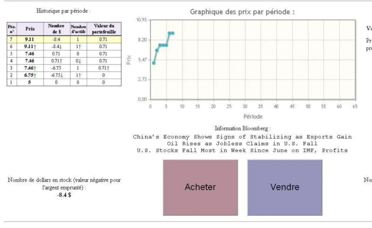
The experiments werecarried out at the Laboratory of Experimental Economics in Paris (LEEP, http://leep.univ-paris1.fr/accueil.htm). Each experiment had two parts: i) participants took part in alottery-choice experiment,described in Section2.2,and ii) participants tradedin a financial market,discussed in Section2.3. The lottery-choice experiment was introduced to assess the risk profile of the participants. A screenshot of the setup for the financial market experiment is shown in figure 1.
2.1.Participants
The experiments took place at the experimental economics laboratory at the Centre d’Economie de la Sorbonne. All experiments were carried outwith students who had doneat least 4 years of economics at the Université Paris 1 Pantheon - Sorbonne. Each participant was only allowed to take part in one experiment.
The total gain of the students included 3 parts: (i) 5 eurosjust for attending the experiments. (ii) Any gains from the lottery-choice experiments.
(iii) Any gains from investing in the financial market experiments.
It should be noted that losses were not allowed in either (i) or (ii), i.e., the worst case scenario for a student would the 5 euros obtained by just taking part in the experiments.
2.2 Lottery-choice experiment
The aim of thelottery-choice experiment was to calculate the risk profile of the participants in each group. The idea behind these experiments was originally proposed by Holt and Laury (2002). The payoff of the lottery-choice experiment is shown in Table 1.
Table 1Payoff in the lottery-choice experiment. For each line,the student chose between Option A and Option B.
Decision Option A Option B
1 1/10 to gain 8 euros, and 9/10 to gain 6.4 Euros
1/10 to gain 16.4 Euros, and 9/10 to gain 0.4 Euros 2 2/10 to gain 8 Euros,
and 8/10 to gain 6.4 Euros
2/10 to gain 16.4 Euros, and 8/10 to gain 0.4 Euros 3 3/10 to gain 8 Euros,
and 7/10 to gain 6.4 Euros
3/10 to gain 16.4 Euros, and 7/10 to gain 0.4 Euros 4 4/10 to gain 8 Euros,
and 6/10 to gain 6.4 Euros
4/10 to gain 16.4 Euros, and 6/10 to gain 0.4 Euros 5 5/10 to gain 8 Euros,
and 5/10 to gain 6.4 Euros
5/10 to gain 16.4 Euros, and 5/10 to gain 0.4 Euros 6 6/10 to gain 8 Euros,
and 4/10 to gain 6.4 Euros
6/10 to gain 16.4 Euros, and 4/10 to gain 0.4 Euros 7 7/10 to gain 8 Euros,
and 3/10 to gain 6.4 Euros
7/10 to gain 16.4 Euros, and 3/10 togain 0.4 Euros 8 8/10 to gain 8 Euros,
and 2/10 to gain 6.4 Euros
8/10 to gain 16.4 Euros, and 2/10 to gain 0.4 Euros 9 9/10 to gain 8 Euros,
and 1/10 to gain 6.4 Euros
9/10 to gain 16.4 Euros, and 1/10 to gain 0.4 Euros 10 10/10 to gain 8 Euros,
and 0/10 to gain 6.4 Euros
10/10 to gain 16.4 Euros, and 0/10 to gain 0.4 Euros
The lottery-choice experiment was carried out as follows. First, each participant made a choice between Option A or Option B for each line in the decision table. The system would then randomly pick one of the decision lines (from decision 1 to 10) for each participant. Given the chosen decision line, a lottery would be performed according to the participant’schoice for that line (i.e., either A or B) and the participant would be awarded the outcome of that lottery.
2.3 Trading in a financial market
Whenall students have finished the lottery-choice, their risk profile is known (see section 4.1). They then proceedto the financial market experiment, which is the most important of the two experiments.
The number of participants in each experiment was fixed at10. There was only one asset in our financial market which the participants could either buy or sell, short-selling being allowed(see figure 1). The initial price of the asset was fixed at5 euroswith an expectation of a 10 cent dividend payout at the end of the 60 time periods. Each of the 60 time periods lasted 15 seconds. In each time period, the participants were presented brief statements of economic news and they could either buy or sell ONE asset or do nothing. The participants were told that the asset was correctly priced according to rational expectations (Muth, 1961), that is, the price of the asset was supposed to correctly reflect all future discounted cash flow accrued to the asset. The participants could, at zerointerest rate, borrow money to buy shares, and short-selling was allowed. The parameters in each experiment are shown in Table 2.
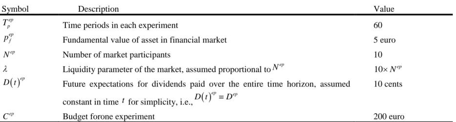
Table 2. Parameters for each experiment.
Symbol Description Value
ep p
T Time periods in each experiment 60
ep f
p Fundamental value of asset in financial market 5 euro
ep
N Number of market participants 10
Liquidity parameter of the market, assumed proportional toNep 10Nep
epD t Future expectations for dividends paid over the entire time horizon, assumed
constant in time t for simplicity, i.e.,
ep ep
D t D
10 cents
ep
The general financial information was taken from real financial news items obtained on Bloomberg over a two week time period. Students were told the asset represented a portfolio of assets like an ETF or an index. They were all simultaneously presented with the same information, meant to reflect general financial news, e.g. good or bad US employment figures, commodity price changes, etc. The news items were the same in all experiments and were chosen without positive or negative bias.
At the end of each time period, the participants’orders were gathered and a new market price calculated (using Eq. (3.3)inSection 3.1), based on the order imbalance (with sign and magnitude determining the direction andsize of the price movement).This was thenshown to the participants graphically on their computer screen. Throughout the experiment the participants had a continuous update of the number of shares held and their gains/losses.
At the end of each experiment, a pool of 200euro was distributed pro rata among the participants who had a positive excess gain.
3 Simulation Approach
The simulation method used was the so-called “$-Game”, a multi-agent based modeling approach (Vitting-Andersen, and Sornette, 2003), in which each individualagent makes his/her investment decisions with the aim of maximizing their profit payoff function. The objective was to detect the speculative and fundamental states in the experimental market data.The $-Game was inspired by the Minority Game (MG), introduced in 1997 by Yi-Cheng Zhang and Damien Challet (Challet, and Zhang, 1997; Challet, and Zhang, 1998) as an agent-based model to study market price dynamics (Zhang, 1998; Johnson, Hart, and Hui, 1999; Lamper, Howison, and Johnson, 2001). The basic MG scheme consists ofa repeated game where the players choose to buy or sell at each time step on the basis of past information, and the winning partyis the one that selects the minority part. Like the Minority Game, the $-Game should be considered as a “minimal” model of a financial market.
3.1 The $-Game
The mathematical scenario of the $-Game model includes N agents that simultaneously take part in a one-asset financial market over a time horizon of Tp
periods. In each time period t , with tTp, each agent i chooses an action
1,0,1
i
a t , where the action 1 is a “sell” order, the action 1 is a “buy” order, and the action 0 is a “hold” order, which means neither “buy” nor “sell”. Players are assumed to be bounded rational, in the sense of using only a limited information set to make their decisions, with no short-sale constraints. In the version of the $-Game presented in this study, the agents use two different types of investment strategies: (i) technical analysis strategies and (ii) fundamental analysis strategies.
3.1.1 Technical analysis strategies
Concerning decision-making based on technical analysis, each player observes the history of past price movements, which is limited to the size of their memory,
m . Therefore, m denotes the size of the agent’s memory. Each agent has a fixed number of strategiess. These s strategies are chosen randomly among the total pool of strategies (see below) and are assigned at the beginning of the game. A specific strategy j tells whether to buy, sell, or hold an equity depending on the past price history of up moves, represented as “1”, and down moves, represented as “0”.
In each time period t , the ith agent uses his/herbest strategy to take an action
*
i
a t of buying a ti*
1, or selling a ti*
1, or simply doing nothinga ti*
0. The superscript* is used to mark a t is the optimal strategy at time t. i
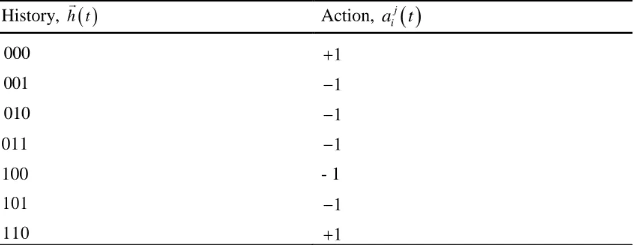
Table 2Example of a strategy.
History, h t
Action, aij
t 000 1 001 1 010 1 011 1 100 - 1 101 1 110 1111 0
A strategy tells an agent what to do given the past market behavior. Table 2 shows an example of a strategy form3. For all possible histories of up and down market moves over the last m time steps, the strategy suggests a specific action to take at time t , namely aij
h t
1, 0, 1 with h t
0,1 m.For instance, if the market went down over the last 3 days, the strategy in Table 2 suggests buying the stock (000 1). If instead the market first went up, then down and finally up, the same strategy suggests selling(101 -1). Notethat, since the price has 2 possible moves (up or down), the number of possible price paths equals2m8 bit sequences of 0’s and 1’s, each corresponding to a specific action
1,0, 1
suggested by the j strategy. This meansthat the space of all possible strategies is given by 23m 6561.
Agents keep a record of the overall payoff for each strategy over the entire market history (i.e., not limited to m past periods) using a rolling window of size m , and use this record to update which strategy is the most profitable at a given time t. This renders the game highly non-linear: as the price behavior of the market changes, the best strategy of a given agent changes,and this canthen lead to furtherchanges in the price dynamics.
The original $-Game payoff function of the ith agent’s jth strategy aij
t inperiod t is determined by
1
j j i i a t a t r t (3.1)where r t denotes the return of the market between time
t1 and t .The payoff in the $-Game therefore describes the gain/loss obtained by an investment strategy executed at time t1 depending on the market return in the following time step t . As shown byChordia, Roll, and Subrahmanyam (2001) and Chordia, and Subrahmanyam (2004), the actions of traders significantly impact price returns and liquidity through a positive autocorrelation in equilibrium. Imbalances in the order book thereby reflect a positive relation between imbalances and future returns. The price returnr t from
t1 to t can therefore be assumed to be proportional to the order imbalance, leading to
ln
ln
1
A t
r t p t p t
(3.2)
wherep(t) denotes the price of the stock at time t. Given a certain order imbalance, the market price p t can be calculated as
1 A t
p t p t e (3.3)
whereA t indicates the global order imbalance (see Eq.(3.4)) and
is a parameter describing the liquidity of the market, withN. The price goes in the direction of the sign of the order imbalance (Holthausen, Leftwich, and Mayer, 1987; Plerou, Gopikrishnan, Gabaix, and Stanley, 2002) and
*
1 N k k A t a t
(3.4)Therefore, the payoff function in Eq.(3.1) can be re-expressed in terms of the return function in Eq.(3.2) as
* 1 1 1 N k j j j k i i i a t A t a t a t a t
(3.5)To summarize, in the $-Game technical analysis, trading strategies are based on a reward scheme for strategies whichat time t1 predicted the rightdirection forthe return of the market r t in the next time step t . The larger the marketmovement, the
more the loss or gain depends on whether the strategy correctlyor incorrectlypredicted the market movement.
In order to understand the findings of our experiments, we then extended the $-game to include that fact that people are risk averse. Rather than being concernedsolely about absolute gains or losses, investors also pay attention to the risk involved in obtaining a certain level of profit. In finance, the Sharpe ratio is one way
to examine the performance of an investment strategy by adjusting for its risk. We thus rewrite the original $-Game payoff function to include a “Sharpe Ratio”, i.e.,
1
j j i i r t a t a t r t (3.6)where
r t
is the standard deviation of the return r t from the beginning of the
game to time t . Specifically, if there are two ways to obtain a certain return, Eq. (3.6) ensuresthat investors will pick up the strategy which involves the least risk.
Furthermore, it should be noted that people are loss averse (Kahneman and Tversky (1979)). We therefore divide
r t
intoa gain part, denoted by
r
t
, and aloss part, denoted by
r
t
. The payoff function becomes
1 j j i i r t a t a t r t r t (3.7)Here
r
t
is the standard deviation of positive r
t from the beginning of the game up totime t ,while
r
t
is the standard deviation of negative returnsr
tfrom the beginning to time t . andtake into account the asymmetry of gains versus losses. The special case of 0 corresponds to the standard $-game.
3.1.2 Fundamental analysis strategies
In addition to technical analysis strategies that seekto profit from price changes, we also consider strategies that seekto profit from information aboutthe fundamental value of an assetp t . Each player estimatesf
p t by discounting future estimated f
cash flow (dividends) accrued to the asset. In order to limit the sell orders in the case of extreme price deviationsp t
pf
t or p t
pf
t , we assume a vanishing use of the fundamental strategy according to a Poisson process of the form:
, p t pf t e with D t (3.8)This assumption provides a maximum probability bychoosing the fundamental strategy in correspondence with a price variation from its fundamental value that is almost equivalent to the dividend yield. Thismakes sense, given that the fundamental price is the expectation of future dividends.
3.1.3 Market dynamics
The formulation of the decision-making process using the $-Game leads to a financial market model based on the 9 parameters shown in Table 3.
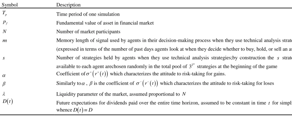
Table 3 Parameters of the financial market model based on the$-Game.
Symbol Description
p
T Time period of one simulation
f
p Fundamental value of asset in financial market N Number of market participants
m Memory length of signal used by agents in their decision-making process when they use technical analysis strategies (expressed in terms of the number of past days agents look at when they decide whether to buy, hold, or sell an asset)
s Number of strategies held by agents when they use technical analysis strategies;by construction the s strategies available to each agent arechosen randomly in the total pool of 2
3m strategies at the beginning of the game Coefficient of
r
t
which characterizes the attitude to risk-taking for gains. Similarly to, is the coefficient of
r
t
which characterizes the attitude to risk-taking for loses Liquidity parameter of the market, assumed proportional to N
D t Future expectations for dividends paid over the entire time horizon, assumed to be constant in time t for simplicity,
Figure 2 illustrates the price dynamics of the $-Game: i) At each time step, the agents update the score of their different strategies according to the payoff function. ii) Given the actual history of the market, i.e.,h t
, each agent chooses the best performing strategy from the set of s available strategies. iii) Then the best strategy is used to decide whether to buy, hold, or sell an asset and place an order. iv) After each agent places its order, all orders are gathered together. v) This leads to a new price movement of the market: up if a majority choose to buy, and down if a majority choose to sell.Once again, we see from Figure 2 that,as the market changes, the best strategies of the agents change too, and as the strategies of the agents change, they thereby change the market.
Figure 2. Representation of the price dynamics in the $-Game. Agents first update scores of all their s strategies depending on their ability to predict the market movement. After scores have been updated, each agent chooses the strategy which now has the highest score. Depending on what the price history happens to be at that moment, this strategy determines which action a given agent will take. Finally, the sum of the actions of all agents determines the next price move: if positive, the price moves up, if negative, the price moves down.
3.2 Decoupling and synchronization
Under certainspecific market conditions, it is possible that,regardless ofthe future states of the market, the investor’s strategy will always recommend a given decision. In such situations, the decision is independent of what will happen next. An investor is no longer influenced by the incoming information because all information will drive them to the same conclusion, making the market predictable. This cognitive mechanism is called “decoupling” in our paper.
Let hm
t indicate the price history of the last m movements at time t . A strategy is called (one time step) “decoupled”, if the action of the strategy at timet2 , denoted bya h
m
t2
, does not depend onhm
t1
. On the contrary, a strategy is said to be coupled to the price history if a h
m
t2
does depend on the outcome of
1
m
h t (Andersen, and Sornette, 2005).
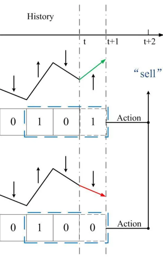
The strategy shown in Table 2 is one-time-step decoupled when conditioned on the price history hm
t 010
at time t . This holds because, no matter what price movementoccurs at timet1 (up/down), the strategy will always recommend to sell at time t2(see Figure 3).Figure 3. Illustration of one-time-step decoupling for the strategy shown in Table 2 in the case of a price history of (010).One-time-step decoupling means that, no matter what price movement occurs at time t1(0 or 1), the strategy will recommend the“sell” action at timet2.
This means that so long as we see an occurrence of the price history where the market first went down (0), then up (1), then down (0), we know for sure this strategy will recommend “sell” (-1) two time steps ahead. In a hypothetical game with only one agent and only the one strategy presented in Table 2, given the price history (010), we would therefore know with certainty what the agent would do two time steps ahead.
So far we have showed how an analysis of the agents’ strategies could lead to momentary predictability of their future actions. But knowing for sure what one, or even several agents will do, does not guarantee being able to predict what will happen at the level of the market. To know how the market will behave, we need to encounter a situation in which, not only are a majority of agents decoupled, but they need to be decoupled in the same direction. At any time t , the actions of agents can be thought of as coming from either coupled or decoupled strategies. The order imbalance can be rewritten as h t h t h t coupled decoupled A A A (0.1)
The condition for certain predictability of what will happen one time step ahead is
2 2 h t decoupled N A t (0.2)The sign of the price movement at time t2 will be determined by the sign of
2 h t decoupled A t for a given price history at time t .Adecoupled is used to record the decoupled strategies with actions 1, whileAdecoupled is used to record the decoupled strategies with actions 1.
Decoupling of a strategy means that different patterns of market history lead to the same decision (i.e., buy or sell), regardless of whether the market went up or down in the time step preceding the one in which the decision is to be made. The most interestingpoint about the decoupling mechanism is that it gives a handle to predict biased price behavior before it can be seen in the price data.
4 ExperimentalResults
4.1 Experimental design
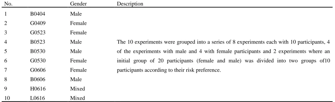
We performed a series of 10 experiments, as listed in Table 4. The parameters of each experiment can be found in Table 2, Section 2.
Each experiment included10participants.,In experiments 1 to 8, the participants were either men orwomen. Experiments 9 and 10 weredone differently. First, agroup of 20 participants, men and women, were tested for their risk preferences. The group of 20 was then divided into two groups according to their risk preference. The participants in H0606 were greater risk-takersthan the participants in L0606.
Table 4. A list of experiments performed in our study.
No. Gender Description
1 B0404 Male
The 10 experiments were grouped into a series of 8 experiments each with 10 participants, 4 of the experiments with male and 4 with female participants and 2 experiments where an initial group of 20 participants (female and male) was divided into two groups of10 participants according to their risk preference.
2 G0409 Female 3 G0523 Female 4 B0523 Male 5 B0530 Male 6 G0530 Female 7 G0606 Female 8 B0606 Male 9 H0616 Mixed 10 L0616 Mixed
4.1.1 Lottery-choice results
In order to ascertain therisk profile of the trader population, we did alottery-choice experiment before the financial market experiment. The lottery-alottery-choice payoff is based on ten choices between the paired lotteries in Table 1. As mentioned before, the options B are riskier than the options A. Let’s focus for a moment on the first decision in the lottery-choice table. The expected return of option A, i.e.,rAe
1 6.56 euro, is much bigger than the expected return of option B, i.e., e
1 1.9A
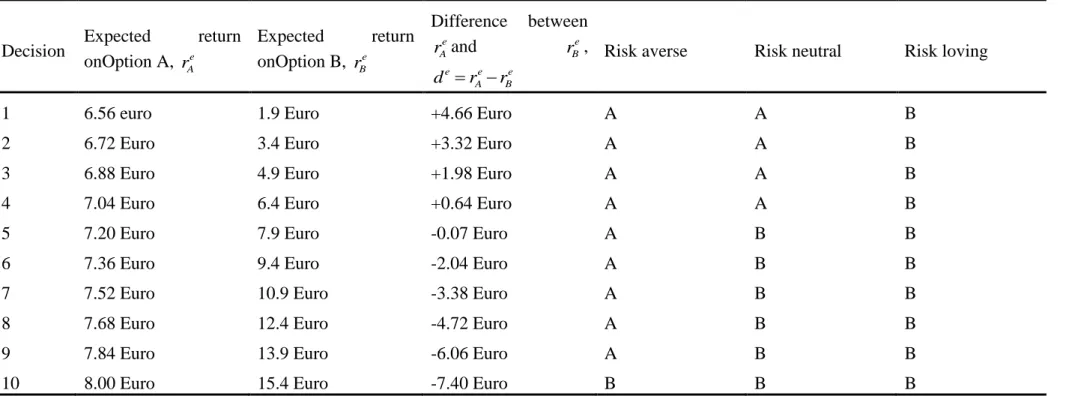
r euro. So most people would choose option A, except for extreme risk seekers, who would choose option B. In contrast, if we focus on the ninth decision, most people would chose option B, except for an extreme risk-averse person, who would choose option A. When the probability of ahigh payoff outcome increases sufficiently, a participant should switch from option A to option B. In the three right-hand columns of Table 5, three different risk profiles are shown. A risk-neutral person would choose A fordecisions 1 to 4 and then switch to B. Notice that even the most risk-averse person should switch to B by decision 10, since option B gives a sureprofit of 15.4 euros.
Table 5. Expected return onten paired lottery-choice decisions and 3 examples of choices for risk-loving, risk-neutral, and risk-averse players.
Decision Expected return onOption A, e A r Expected return onOption B, e B r Difference between e A r and e B r , e e e A B d r r
Risk averse Risk neutral Risk loving
1 6.56 euro 1.9 Euro +4.66 Euro A A B
2 6.72 Euro 3.4 Euro +3.32 Euro A A B
3 6.88 Euro 4.9 Euro +1.98 Euro A A B
4 7.04 Euro 6.4 Euro +0.64 Euro A A B
5 7.20 Euro 7.9 Euro -0.07 Euro A B B
6 7.36 Euro 9.4 Euro -2.04 Euro A B B
7 7.52 Euro 10.9 Euro -3.38 Euro A B B
8 7.68 Euro 12.4 Euro -4.72 Euro A B B
9 7.84 Euro 13.9 Euro -6.06 Euro A B B
Ten lottery-choice experiments were carried outin our study, each involving 10 participants, giving in total the risk profiles of 100 participants. We found that only 2 of the participants were extremely risk-loving,one in experiment B0404 and the other in experiment H0606. Interestingly, the 2 extreme risk seekers were male. On the other hand, we found 7 of the 100 participants to be extremely risk averse.
1
2
Figure 6.Four experiments performed with women.
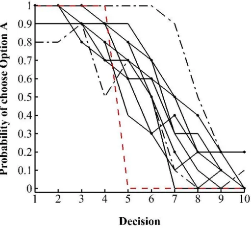
Comparing Figures 4-6, the women in our experiments were clearly more risk averse than the men. In all the experiments with women, the first decision choices (1 and 2) were always A, whereas this was not the case with the groups containing men. Two of the groups of men had a probability of only 0.9 of choosingA for decision number 1. In addition, for men, the probability of choosing Option A declined faster versus the decision number. That is, male traders crossed over to Option B earlier than female traders. Women seek a higher payoff only if the probability of earning a higher payoff is large enough. In order to quantify risk profile by gender, we calculated the median of the probability of choosing option A(see Table 6 below).
Table 6. The median probability of choosing option A for each experiment.
3 B0404 Male 4.75 G0409 Female 7.00 G0523 Female 6.00 B0523 Male 6.00 B0530 Male 6.33 G0530 Female 5.33 G0606 Female 7.00 B0606 Male 6.50 H0616 Mixed 6.00 L0616 Mixed 8.00
4.1.2 Financial market results
Each group of participants performed 60 periods of trading in the financial market system introduced in Section 2. Figures 7 a)-d) showthe market prices generated by the 10 groups. The horizontal axis shows the time period and the vertical axis the market price. The solid line shows the experiments with male traders (B0404, B0523, B0530, and B0606) and the solid line with circles the experiments with female traders (G0409, G0523, G0530, and G0606). The dashed line presents the last 2 experiments where an initial group of 20 participants (female and male) wasdivided into two groups according to their risk preference.
4
5
6
7
8
One notes an extraordinary price growth in some cases. In others, however, the market price merely fluctuated around the fundamental value. In order to identify the market behavior, three typical market states: “speculative state”, “fundamental state”, and “other state” were defined (see Table 7). A speculative state is determined by prices exceeding a 200 percent range with respect tothe fundamental value. A fundamental state is characterized by price fluctuations within a 50 percent range of the fundamental value. “Other state” means neither speculative nor fundamental.
Table 7. Definition of market behavior.
State Description
Speculative state p
2pfFundamental state 0.5pf p
1.5pfOther state Neither speculative nor fundamental
Table 8.Market behavior ineach experiment.
Gender State B0404 Male Speculative G0409 Female Speculative G0523 Female Speculative B0523 Male Other B0530 Male Fundamental G0530 Female Fundamental G0606 Female Fundamental B0606 Male Fundamental H0616 Mixed Fundamental L0616 Mixed Fundamental
Three of the ten experiments created “bubbles”, six fluctuated around the fundamental value the whole time, and only one belongs neither to the speculative nor to the fundamental state. The result of oneexperiment, B0404, was quite particular. It was a “super bull” case
9
where the final market price exceeded the initial fundamental value by a factor of 20. This experiment was performed with a group of male traders. It was also the most risk-seeking group, with a medianof 4.5 to choose option A, the smallest median in all the experiments.
In order to understand and quantify the risk-taking behavior of the participants in the market experiments, we then turned our attention to the probability distribution for the gain/loss ΔW incurred during one trading period in the market experiment.We therefore calculated the full width at half maximum (FWHM) of the gain/loss probability distribution. Figure 8 shows how to get the FWHM from a given distribution. The FWHM consists of FWHM+ and FWHM-, which are also illustrated in Figure 8:
FWHM FWHM FWHM (4.1)
W
can be obtained from
1i i
W W t W t
(4.2)
10
One way to quantify the experimental results is therefore to use the FWHM to get a risk profile of each group. Figures 9 a)-b) show the probability distribution of W for two typical experiments performed with men (a) and women (b).Table 9 lists the FWHM of the probability distribution of W for all 10 experiments. In most instances, the FWHM values for thewomen’s groups were smaller than those forthe men’s groups. This illustrates the observation that women seemed more “cautious” than men when they were trading. It is also onereason why the price movements in the women’s experiments seem less extreme. However, a surprising thing was that two groups of female traders who were individually risk averse(as seen from the FWHM) created excessive risk-takingcollectively (G0409 and G0523). Comparing the FWHM values with male groups, the female groups took fewer risks. This means that female tradersmanaged to createexcessive risk at the market level justby taking only small individual risks.
Table 9. The FWHM of each experiment
Gender FWHM+ FWHM- FWHM B0404 Male 24.8459 -8.0755 32.9214 G0409 Female 0.2098 -0.9460 1.1558 G0523 Female 0.1223 -0.2349 0.3572 B0523 Male 1.6767 -1.4597 3.1364 B0530 Male 1.9224 -1.8255 3.7479 G0530 Female 0.1830 -0.2667 0.4497 G0606 Female 0.5702 -0.9265 1.4967 B0606 Male 0.5458 -0.3983 0.9441 H0616 Mixed 0.1967 -0.2398 0.4365 L0616 Mixed 0.8771 -0.5569 1.4340
11
Figure 9 a) Probability distribution of ΔW for the experiment B0404.
12
5 Simulation Results
5.1 Macroscopic simulation analysis
In order to understand the experiments, Monte Carlo (MC) simulations with various parameters were carried out. The MC simulations were used to calculate the probability ofexcessive risk-taking.
We first introduce a “temperature” to analyze the experiments and set up a general theoretical framework giving a broad insight into the experiments. The “temperature”T
wasintroduced by Savona, Soumare, and Vitting Andersen (Savona R, Soumare M, and Andersen JV (2015)). It can be related to Ginzburg-Landau theory (GL theory). One of the main implications of the GL theory is the existence of a nontrivial transition from a high “temperature” disordered state in the trading experiments, where traders do not create a trend over time, to a low “temperature” state characterized by trend following. Asin (Savona, Soumare, and Vitting-Andersen),we defineT by
2m 1 T N s (5.1)
First, we note that the qualitative behavior of a trading experiment can be predicted if we are given the market temperature T for fixed memory length m . This means that, no matter how many market participants N there are, and how many strategies s there are for each participant, if the market temperature T and memory length m are fixed, the macro behavior will be similar. Second, the memory length seems to play a major role in moving the system between the two states of speculative and fundamental behavior. The larger the value of m , for the same temperature, the more fundamental the behavior.
13
Figure 10 Probability of creating a speculative state as a function of market temperature T for 2,3, 4,6
14
From Figure 10, one can see that the probability of creating a speculative state decays with T. One notes that, for each m (2, 3, 4, or 6), the probability of creating a speculative state is highest when the market temperature T is lowest. Second, the greater the length of memory m, the smaller the probability of creating a speculative state. Third, the smaller the value of m, the faster the probability of creating a bubble decreaseswith T.
5.2 Microscopic simulation analysis
We then used game theory and computer simulations as a theoretical framework to understanding excessive risk-taking via the price formation in eachof the experiments performed. Having carried outthe trading experiments with human subjects, the outputs from the experiments in terms of a price time series wereused as input to agent-based Monte Carlo (MC) simulations of the $-Game.
The MC simulations were performed with fixed Tp and N corresponding to the
experiments. The memory length m was selected randomly from 2 to 5. The number of strategies s was selected randomly from 2 to 10, with random initial realization of each of the
s strategies. Table 10 shows the parameters used in MC simulations. We used the price data
generated from experiment B0404 as input price data, and 100 randomly generated MC realizations were then used to make an average estimate of Adecoupled and Adecoupled .
Table 10 Parameters used in microscopic MC simulations.
Symbol Value p T TpTpep60 f p ex 5 f f p p N ep 5 N N m A random number, 2 m 5 s A random number, 2 m 10 1 4 4 10 N
D t D t
Dep10.15
Figure 11 shows Adecoupled (solid lines) and Adecoupled (dashed lines) over time. Adecoupled
indicates the optimal strategies in the MC simulation decoupled along the direction of the price increase, whereas Adecoupled indicates the optimal strategies against the direction of the price increase. Before the market price in experimentB0404 began to increase rapidly, we observe a split between theAdecoupled strategies and theAdecoupled strategies. Although Adecoupled
was not over N/ 2, the trend in theprice movement formed when the split became stable. This is one illustration of how speculative behavior can be detected (via the decoupling parameters) before it is seen in the price dynamics.
Figure 12 shows the microscopic MC simulations applied to experiment G0530. Again there appears to be a small but constant split between theAdecoupled strategies and theAdecoupled
16
17
18
6 Conclusion
Financial market experimentswere performed usinggroups of either men or women, as well as groups having a different composition of risk profile. The risk profile of participants was obtained from a lottery-choice experiment prior to the financial market experiment. In the financial market experiment, both fundamental value behavior and speculative behavior were observed. The main question we have tried to answer in this paper is this: given the same financial news announcements, how come one observes fundamental value behavior in some experiments, and speculative behavior in others. This study introduced a variant of the$-Game to understand the origins ofexcessive risk-taking as formedin collective decision-making. Froma macro perspective, the probability of speculative behavior was shownto depend on the market temperatureT , the memory length m , and therisk profile. The probability of creating
a speculative state is higherwhen the market temperature is lower. The greaterthe memory length, the smaller the probability of creating a speculative state.From a micro perspective, the trend in theprice movement formed (speculative state) when the split between the Adecoupled
strategies and theAdecoupled strategies became stable. This means that the spilt betweenthese strategies can be used to predict the market state before it is observed in the price dynamics.
19
The research leading to these results has received funding from the European Union SeventhFramework Programme (FP7-SSH/2007-2013) under grant agreement no. 320270 SYRTO. This work was carried out in the context ofthe Laboratory of Excellence on Financial Regulation (Labex ReFi) supported by PRESheSam under the reference ANR-10-LABX-0095. It benefitted from French government supportmanaged by the National Research Agency (ANR) as part ofthe project Investissements d’AvenirParis Nouveaux Mondes (invesiments for the future, Paris-New Worlds) under the reference ANR-11-IDEX-0006-02.
References
Andersen J V, Nowak A. An Introduction to Socio-Finance. Springer, Berlin(2013).
Andersen J V, and Sornette D. A mechanism for pockets of predictability in complex adaptive systems. Europhysics Letters, 70(5): 697 (2005).
Barber B M, Odean T. Boys will be boys: Gender, overconfidence, and common stock investment. Quarterly journal of Economics, 2001: 261-292.
Challet D, and Zhang Y C. Emergence of cooperation and organization in an evolutionary game. Physica A: Statistical Mechanics and its Applications, 1997, 246(3): 407-418.
20
Challet D and Zhang Y C. On the minority game: Analytical and numerical studies[J]. Physica A: Statistical Mechanics and its Applications, 1998, 256(3): 514-532.
Chordia T, Roll R, and Subrahmanyam A. Order imbalance, liquidity, and market returns. Journal of Financial economics, 2002, 65(1): 111-130.
Chordia T, and Subrahmanyam A. Order imbalance and individual stock returns: Theory and evidence. Journal of Financial Economics, 2004, 72(3): 485-518.
Coates J M, Herbert J. Endogenous steroids and financial risk taking on a London trading floor. Proceedings of the National Academy of Sciences, 2008, 105(16): 6167-6172.
Coates J M, Gurnell M, Rustichini A. Second-to-fourth digit ratio predicts success among high-frequency financial traders. Proceedings of the National Academy of Sciences, 2009, 106(2): 623-628.
Coates J M, Page L. A note on trader Sharpe Ratios. PloS ONE, 2009, 4(11): e8036.
Holt C A, Laury S K. Risk aversion and incentive effects. American Economic Review, 2002, 92(5): 1644-1655.
Holthausen R W, Leftwich R W, Mayers D. The effect of large block transactions on security prices: A cross-sectional analysis[J]. Journal of Financial Economics, 1987, 19(2): 237-267.
Johnson N F, Hart and M, Hui P M. Crowd effects and volatility in markets with competing agents. Physica A: Statistical Mechanics and its Applications, 1999, 269(1): 1-8.
21
D. Kahneman, A. Tversky, Prospect theory: an analysis of decision-making under risk.Econometrica 47(2), 263–292 (1979)
Kirman A. Epidemics of opinion and speculative bubbles in financial markets. Money and financial markets, 1991: 354-368.
Lamper D, Howison S D. and Johnson N F. Predictability of large future changes in a competitive evolving population. Physical Review Letters, 2001, 88(1): 017902.
Markowitz H M. Portfolio selection: efficient diversification of investments. Yale University Press, 1968.
Muth J F. Rational expectations and the theory of price movements. Econometrica: Journal of the Econometric Society, 1961: 315-335.
Plerou V, Gopikrishnan P, Gabaix X, et al. Quantifying stock-price response to demand fluctuations. Physical Review E, 2002, 66(2): 027104
Savona R, Soumare M, and Andersen JV (2015) Financial Symmetry and Moods in the Market. PLoS ONE 10(4): e0118224. doi:10.1371/journal.pone.0118224
vanStaveren I. The Lehman Sisters hypothesis. Cambridge Journal of Economics, 2014: beu010.
Vitting Andersen J, Sornette D. The $-game. The European Physical Journal B-Condensed Matter and Complex Systems, 2003, 31(1): 141-145.
Zhang Y C. Modeling market mechanism with evolutionary games. arXiv preprint cond-mat/9803308, 1998.