HAL Id: halshs-00113342
https://halshs.archives-ouvertes.fr/halshs-00113342
Submitted on 13 Nov 2006
HAL is a multi-disciplinary open access
archive for the deposit and dissemination of sci-entific research documents, whether they are pub-lished or not. The documents may come from teaching and research institutions in France or abroad, or from public or private research centers.
L’archive ouverte pluridisciplinaire HAL, est destinée au dépôt et à la diffusion de documents scientifiques de niveau recherche, publiés ou non, émanant des établissements d’enseignement et de recherche français ou étrangers, des laboratoires publics ou privés.
To cite this version:
Centre d’Economie de la Sorbonne
UMR 8174
Wage and employment in a finance-led economy
Célia FIRMIN
Wage and employment in a finance-led economy
∗Célia Firmin1
MATISSE
Centre d’économie de la Sorbonne : UMR 8174 CNRS et Université Paris 1 Panthéon-Sorbonne
Abstract: The object of this paper is to analyse the links between income distribution and growth in a finance-led economy, with a post Keynesian “stock-flow” macroeconomic model. In fact, the increased share of financial activities creates a new macroeconomic and income distribution dynamic. We will use the steady-state case and simulations experiments to analyse model reaction to a change in financial key parameter when the wage share is endogenous.
Keywords: financialization, labor’s share, capital accumulation, simulations experiments
Salaire et emploi dans une économie financiarisée
Résumé : Ce papier a pour objectif d’analyser les liens entre répartition des revenus et croissance dans une économie financiarisée par le biais d’un modèle macroéconomique Postkeynésien de type « stock-flux ». L’accroissement de la part des activités financières s’accompagne de nouvelles dynamiques macroéconomique et de distribution des revenus. Nous utiliserons des simulations numériques afin d’analyser les réactions du modèle à une modification des variables financières dans le cadre d’une détermination endogène de la part des salaires.
Mots-clés : financiarisation, part salariale, accumulation du capital, simulations Codes JEL: E12, E24, E44, E51
∗ Une version préliminaire de ce texte a fait l’objet d’une communication au Goodwin Workshop,
organisé à l’Université de Brême les 10-12 novembre 2005, lors du colloque de l’EAEPE
Introduction
The object of this paper is to analyse the links between income distribution and growth in a finance-led economy. To study these links, and employment, in finance-led economies, we will use a post Keynesian “stock-flow” macroeconomic model. This kind of model is developed by Godley and Lavoie (2001). These models are generally specified by a Kaleckian wages determination, by a mark-up rule in goods market. Here, we will introduce an endogenous wage determination lead by class struggle, as Goodwin (1967). We will still deal with a markup rule and take into account financial actors. The Goodwin model takes place in a classical framework, where saving affects investment and where there is no demand constraint. On the contrary in a Kaleckian or Keynesian framework, saving and investment don’t respond to the same determinants and the causal relation is reversed. So, the object of this paper is to introduce an endogenous wage determination in a Keynesian model, with a demand constraint but also with an investment financing constraint, in a finance-led economy. Moreover, there is no saving constraint in our model. But, money plays a central part and credit rationing can decrease investment. As Keynes (1937) said, a lack of liquidity can occur, but not of saving. Finance development affects banks behaviour and then credit access by modifying their liquidity preference.
To consider modern finance-led economies specifications, we will introduce financial and credit markets but also speculative assets market, as Taylor (1991). We will present the model by markets in a first time. Then, we will analyse wages and employment determination in a finance-led economy, in comparison to this of Goodwin (1967) model. We will also see the relationship between income distribution and cycles in a finance-led economy, always in comparison to Goodwin model. Finally, we will use simulations experiments to analyse model reactions to a change in key parameters, and mainly a change in financial parameters. More precisely, we will see what the relationships between wages determination and economic dynamic are in a finance-led economy.
1. Model presentation
The model purpose is to introduce an endogenous wage determination, outside the goods market, as Goodwin (1967), in a post Keynesian model but also to consider finance
development and credit rationing. For this, we will introduce financial profitability norms in the investment function and dividends distribution to shareholders. This last modify the consumption function. So, with dividends and interest payments, all profits are not invested. To achieve this, we will not consider the total profit share in the investment function, on contrary to Goodwin, but only anticipated profits linked to economic activity. Firms can finance their investments by issuing equities, borrowing from banks and by retained earnings.
In this model, there are five agents: workers households, shareholders, firms, banks, and an external agent (foreign countries for example). It is composed by five markets: goods market, equities market, credit and money markets and speculative assets market. Accountable matrices are presented in annexes. Exponents in variables represent the demand (d) or the supply (s) and the indexes the agents (a for shareholders, w for workers, f for firms, b for banks and e for external agents).
1.1. Goods market
The production level is determined by aggregate demand, s d d
I C
Y ≡ + . It represents the
total income which is divided between profits and wages. This income distribution influence next period consumption and investment.
1.1.1. Consumption function
We will consider two kinds of consumers:
w a d C C C = +
As Taylor (1991), we first consider wage-earning workers with a propensity to consume equal to one. The second part represents the shareholders. Their income is only constituted by dividends and interests on deposits. This is a simplification but it doesn’t really modify analysis results.
Workers households consume wages of previous period:
) 1 (− ⋅ = W Cw α
Shareholders hold interests on deposits and dividends. In counterpart they consume following their propensity to consume and they save:
) ( ( 1) d( 1) a m d a a D r M C =β⋅ − + ⋅ − With d a
D (−1)dividends received at the previous period, rm⋅Mad(−1)interest on deposits andβ the propensity to consume.
Dividends are determined following the stock of equities hold by shareholders households ( d
a
e ) and the equities rate of return (r ): e Dad =re⋅ead(−1) andead =ead(− )1 +∆ead,
with s f s f e e D
r = , dividends distributed by firms (Dsf ) on the stock of equities issued (esf ). The rate of return on deposits is exogenous, rm =rm .
1.1.2. Investment function
On contrary to Goodwin (1967), we will not consider that profitability affects investment. The profitability level is an indicator of firms’ internal financial possibilities. Yet, firms distribute dividends and pay interest on loans. So, retained earnings represent a better indicator of firms’ income than the profits share. But, these variables don’t enter in firms’ investment decision but in firms financing capacities. So, we will make a difference between firms’ investment decision according to economic activity and financial norms and investment financing conditions. Yet, these last can limit the investment, we will see this point with the credit market.
The demand level influences the investment. Goodwin (1967) model doesn’t take into account the demand effect on investment, as N.Canry (2005) underlines. To analyse this effect, we will consider the rate of capacity utilisation, as most of post Keynesian models (Godley and Lavoie 2001, Taylor 1991).
In a finance-led economy anticipated returns on investment, represented by the economic activity evolution, are compared with financial profitability norms and no more with interest rates as Keynes (1936). Because of uncertainty, past and present facts play an important part in firms’ decision and tend to replace anticipated events. Keynes (1936) developed this idea of past and present facts prevalence in investment decisions. Firms invest only if anticipated returns are equal to a certain norm. With financial activities development,
this norm is now set up on financial markets. Boyer (2000) also introduces financial norms in the investment function. If the anticipated return is inferior to the financial profitability norm, firms will not invest. High financial profitability norms create increasing investment selectivity. We will see later firms behaviour in the speculative asset market when investment opportunities are weak.
We can now present the investment function:
) 1 ( ) 2 ( ) 1 ( 0 ) 1 ( ) ( − − − − ⋅ + − ∆ ⋅ + = b u Y Y a i K Id ρ With ) 2 ( ) 1 ( − − ∆ Y Y
economic activity fluctuations of previous period, ρfinancial profitability norms and
K Y u
⋅ =
µ the capacity utilisation ratio, with µ the productivity. We
will consider equally the capital depreciation:Kt = Kt−1
(
1−δ)
+It, with δ the depreciationrate.
Firms can finance their investment by retained earnings but also by issuing equities and contracting loans. We will see that the real investment can differ of the one established by the investment function.
1.2. Equities market
Equities are issued by firms. They finance by this mean a percentage x of their investment which is not covered by retained earnings (Sf(−1)), regardless to the price of equities. This
formulation is inspired by Godley and Lavoie (2001) and Kaldor (1966). A lag of time is introduced because firms set up their financing structure on previous period because of uncertainty:
[ ]
= ⋅(
(−1) − (−1))
∆ f d s f x I S eRetained earnings are made up by total profits minus distributed dividends ( s f
D ) and interest rate payments on loans ( d
l L
r ⋅ (−1)), plus return on speculative assets that firms can hold
( d
f z Z
d f z d l s f T f F D r L r Z S = − − ⋅ (−1) + ⋅ (−1)
With FT =Y −W . The rate of return on speculative assets (Z) is exogenousrz = . rz
Distributed dividends are a percentage of previous period profits once interest (r ) on l
loans ( d f L ) are paid:
(
d)
f l T s f F r L D = χ⋅ (−1) − ⋅ (−1)Shareholders households, banks and external agents compose the demand for equities. Shareholders households wish to acquire a certain proportionγ of equities with their 1 saving but this proportion is modulated by the relative rates of return on equities ( )r and on e
bank deposits (r ) : m
[ ]
(
e m)
a d a r r S e = + − ⋅ ∆ γ1 γ2With S their saving:a a
d a m d a a D r M C S = + ⋅ (− )1 − and ad d a d a M M M = (− )1 +∆ .
Banks use their unused funds with loans granted to acquire equities or speculative assets. They decide to purchase assets according to their liquidity preference and rates of return. These funds are made up by their internal saving S and deposits b M minus loans s
granted. Yet, banks can be rationed by the amount of equities issued. We will see that in this case they use their funds on the speculative assets market:
[ ]
[
d]
a s f s b s b z e d b r r S M L e e e = + ⋅ − ⋅ +∆ −∆ ∆ −∆ ∆ minγ3 γ4 ( ) ( ); With s m b d z d b s l b r L D r Z r M S = ⋅ (−1) + + ⋅ (−1) − ⋅ (−1), Dbd =re⋅ebd(−1) and ebd =ebd(− )1 +∆ebd.With financial liberalization, if equities issued by firms can not be entirely got by banks and shareholders households, external agents complete the demand:
d b d a s f d e e e e e =∆ −∆ −∆ ∆
1.3. Credit and money markets
Firms decide of their investment behaviour according to the function we have seen. But, they can experience credit rationing due to banks behaviour. In this case, firms’ external financing capacities are not sufficient to fulfil the anticipated investment.
To simplify, we will consider that loans demand is made up by firms only, for investment financing. It represents the exact counterpart of equities issue:
[ ]
=(1− )⋅( (−1) − (−1)) ∆ f d d f x I S LBanks grant loans according to their liquidity preference. In fact, they target a certain capital ratio which corresponds to their liquidity preference (Godley and Lavoie 2004). This ratio ( c
C ) is composed by the ratio of banks own funds on targeted loans (L ): cb
c b b c L OF C = With d b d b s b s b b b OF S M L e Z OF = (− )1 + +∆ −∆ −∆ −∆ and Ls =Ls(− )1 +∆Ls. We will consider here this ratio as exogenous. This ratio is a banks’ prudence behaviour indicator. It represents their confidence in the future (Lavoie 2004). Banks establish a kind of risk self-checking. So, there is an endogenous credit supply rationing (Plihon 1998).
The firms’ financial situation influences loans granted by banks. Banks estimate this situation taking into account the firms’ debt ratio including interest payments. As present situation is unknown, we introduce a lag of one period.
These two components set up the loans supply:
c l c s s b s b C K r C L M S L + ⎟ ⎟ ⎠ ⎞ ⎜ ⎜ ⎝ ⎛ ⎟ ⎟ ⎠ ⎞ ⎜ ⎜ ⎝ ⎛ + + ⋅ − ∆ + = ∆ − − 1 1 ) 1 ( ) 1 (
So, it could have a credit rationing: s d
L
L ≤∆
Banks collect money deposits made by shareholders households: d a s M M =∆ ∆ . Banks
deposits represent the difference between shareholders saving and equities purchasing: d a a d a S e M = −∆ ∆
When banks resources are higher than loans granted and equities purchased, they can get speculative assets.
1.4. Speculative assets market
As Taylor (1991), we introduce a speculative assets market. These assets can be gold, real estates, or external assets for example. In our case, we will take the last one.
Asset speculative supply follows the demand and is set up by external agents:
d s
e Z
Z =∆
∆
Speculative assets demand is composed by firms and banks.
Firms get speculative assets when their total resources are higher than investment opportunities:
[ ]
d d f s f f d f S e L I Z = +∆ +∆ − ∆ (− )1So, their first activity is still investment but when opportunities on the goods market and so anticipated returns are too weak, they develop financial or speculative activities.
With their unused resources, banks acquire speculative assets:
d b s s b d b S M L e Z = +∆ −∆ −∆ ∆
2. Wages and employment
2.1. Wages and employment in Goodwin model
In his 1967 model, Goodwin analyses the links between income distribution and growth. Wages are endogenous and depend on employment rate v (
N L
v= , with L the
employment and N the active population):
uv w w + Ω − = &
High employment rate increases wage share and so reduces profits, which decreases investment and growth. With profit share decreased, growth slows down because of a higher financing constraint for firms. Unemployment increases and a new cycle begins.
In Goodwin model, distributive conflicts play an important role and income distribution is central to analyse cycles. But, this model takes place in a classical framework and financial actors are not considered. As Goodwin (1967), we will introduce an endogenous wage share determination, taking into account distributive conflicts but with financial actors. We will also use a kaleckian mark up rate principle to analyse wages in a finance-led economy.
2.2. Wages and employment in a finance-led economy
Aglietta and Rebérioux (2004) and Boyer (2000) analyse the central part of corporate governance in finance-led economies. This principle gives an important role to shareholders in firms’ management decisions. Financial profitability norms become central in income distribution. So, to introduce shareholders strength in distributive conflict, we have to take these norms into account.
The object here is to make this markup rule endogenous. In fact, in most postkeynesian models, the markup is an exogenous parameter and is set up only on goods market (Godley and Lavoie 2004, Kalecki 1990). Here, the markup rate depends on the difference between financial profitability norms and financial assets rate of return. This difference represents financial actor’s strength. So, the markup rate represents here the distributive conflict between agents. As Goodwin (1967), we will take the employment level as an indicator of workers power. Here, we will use the unemployment rate, ur, instead of the employment rate. So, we can write the markup rate equation:
t e
t p ρ r ur π
π +1 = ⋅( − )⋅ +
When the unemployment rate increases, firms raise their markup rate and wage share decreases. It is the same mechanism when financial norms go up. The unemployment is linked to economic growth, following Okun’s law. The present equation is inspired by Dos Santos and Zezza (2004). The unemployment rate depends on the difference between economic growth and the “normal” rate of growth (Y ). This normal rate is set up by productivity and active population growth. Here, we will consider it as exogenous. So:
⎟⎟ ⎠ ⎞ ⎜⎜ ⎝ ⎛ − ∆ ⋅ − = − − t t t t t Y Y Y ur ur 1 1 ϑ
Income distribution affects consumption and investment, and by this way economic growth. This last determines employment and firms profits and so, income distribution. We will see by simulation method the links between income distribution and growth and if a decrease in wage share improves firms financing capacity and so investment and growth, as Goodwin (1967).
3. Results and experiments
We have solved the model numerically and realised a series of simulation experiments. Two kinds of investment constraints appear. In fact, investment can be limited by effective demand level or by financing condition partly due to credit rationing.
3.1. Cycles and income distribution
With this model, we can find three economic trajectories, whatever the investment constraint form is. The regime can converge towards a steady-state situation, with under-employment stability. The growth rate is close to the natural one, firms can distribute dividends and set up a return rate equal to financial profitability norms and so the markup rate is stable. Wage share and consumption can be stabilized, as investment. In this condition, the unemployment rate is also stationary.
The regime can also follow a cumulative recessive trajectory. It can happen for example when financial profitability norms are too high. In this case, the model is marked by instability. Firms increase the markup rate to raise distributed dividends and so financial assets rate of return. Consumption and utilization rate decrease, as investment, and provokes a fall in firms internal saving. So, investment financing constraint increases, as demand constraint, and the economy follows a recessive trend.
Finally, we can analyse a last situation, with growth cycle. But the relationship between income distribution and growth is not the same as Goodwin (1967) one, even when there is a financing constraint. In fact, if the markup rate increases (when financial profitability norms are higher than financial assets rate of return) and so profit share, firms
distribute more dividends and improve financial assets rate of return. In parallel, growth slows down because of the decrease in wage share. This last provokes a fall in consumption and by this way in investment. Consequently, unemployment rate increases. When assets rate of return is equal to financial profitability norms, or higher, firms are more sensitive to workers demands and markup rate can decrease, even if unemployment is higher. In this case, we can say that wages and employment loose their central role in income distribution dynamics. They seem to be adjustment variables, as growth and accumulation rates. Financial profitability norms, distributed dividends and so financial actors occupy a central part in this dynamic and explain cyclic fluctuations. They represent the first determinant of the markup rate2.
At the opposite of Goodwin, a fall in wage share doesn’t create a recovery of the economy by the increase of investment. On contrary, it tends to depress the activity. We can explain this difference by the introduction of a demand constraint. Even if the economy is under a financing constraint, such a reduction creates a fall in profit due to economic activity deceleration. So, firms’ internal saving decreases and this constraint becomes higher. The causality between profits and investment is reverted referring to Goodwin classical model. Here, we follow Kalecki’s (1966) profit and investment causality. Investment determines profit and not the contrary. We can replace the Goodwin relation between wages, profits and unemployment by a relation between financial norms, markup rate and so profits, and unemployment.
We will see by simulations experiments how the model reacts to a change in parameters, and more precisely, what are the relationships between wages, financial profitability norms, markup rate and unemployment.
3.2. Experiments on financial key parameters
The experiments are led in the case of under-employment stability, when the model solution is stable and leads to a steady-state. First, we will see what consequences have an increase in financial profitability norms. Then, we will analyse a change in distributed
2 We have made an other scenario without the unemployment rate in the markup equation and we find
dividends and in the firm’s equities issuing. With the simulations method, we can only change a parameter at once and analyze local stability. But we can understand why the model generates the results given. The results figures express the economy evolution as a ratio of the steady-state base case. In most cases, the results between the demand constraint regime and the financing one are identical. In the following simulations, the regime is under a financing constraint.
3.2.1. Changes in financial profitability norms
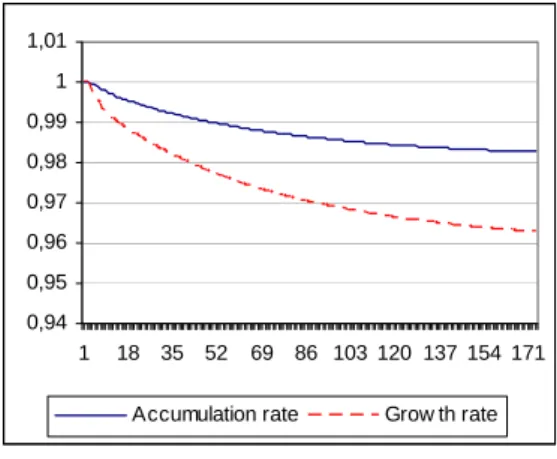
We have seen with the investment function and the markup rate equation that financial profitability norms play a central part in a finance-led economy. It is one of the model key parameter and determines in a large part the kind of regime. In the under-employment and steady-state regime, an increase in financial profitability norms creates a negative effect on growth and accumulation rates. With the chosen parameters, the model sensibility towards a change in ρ is strong and it tends quickly to a depressive state. Here, the model converges to a steady-state where accumulation and growth rates are less important than in the reference case (figure 1a).
Figure 1a: growth and accumulation rates with an increase in financial profitability norms
0,94 0,95 0,96 0,97 0,98 0,99 1 1,01 1 18 35 52 69 86 103 120 137 154 171
Accumulation rate Grow th rate
We can explain this mechanism by the increase in the markup rate which follows higher financial profitability norms. To fulfil financial actors demand, firms have to increase their markup rate in order to raise financial assets rate of return (figure 1b).
Figure 1b: assets rate of return, distributed dividends and markup rate with an increase in financial profitability norms 0,96 0,98 1,00 1,02 1,04 1,06 1 14 27 40 53 66 79 92 105 118 131 144 157 170
Assets rate of return
Distributed dividends on capital Markup rate
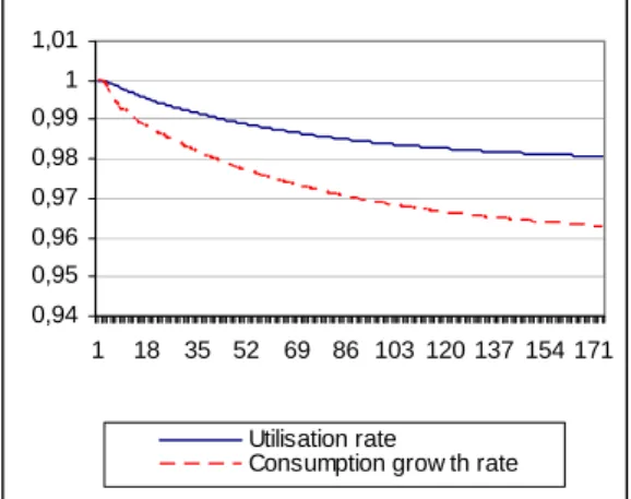
In fact, as the growth decelerates, firms’ profits decrease and the only mean to increase distributed dividends is to increase the markup rate. The wage share decreases (figure 1d) and provokes a fall in consumption and so in utilisation rate (figure 1c). Shareholders consumption is not sufficient to support growth when workers consumption decreases. Shareholders hold a lower propensity to consume and equities are equally held by foreign agents and banks. The equities rate of return is higher than the reference one although profits decrease because firms issue fewer equities with the fall in investment growth.
Figure 1c: utilisation and consumption growth rates with an increase in financial profitability norms
0,94 0,95 0,96 0,97 0,98 0,99 1 1,01 1 18 35 52 69 86 103 120 137 154 171 Utilisation rate
Figures 1d and e: wages share and unemployment rate with an increase in financial profitability norms Wages share 0,991 0,992 0,993 0,994 0,995 0,996 0,997 0,998 0,999 1 1,001 1 16 31 46 61 76 91 106 121 136 151 166 Unemployment rate 0 0,2 0,4 0,6 0,8 1 1,2 1,4 1,6 1 9 1725 334149576573818997 105 113 121 129 137 145 153 161 169
The investment goes down because of the utilisation rate and accelerator effect evolutions. The second cause is the increase of financial profitability norms. In this scenario, we can see that a fall in employment and wages is not followed by a recovery of the activity, even if the economy is under a financing constraint like here and as we have seen in the previous section.
3.2.2. Changes in the distributed dividends ratio
An increase in dividends distributed by firms has a positive effect on accumulation and growth rates despite a first negative shock on accumulation rate (figure 2a). It can be explained by the decrease in firms’ saving when the distributed dividends increase the first year.
Figures 2a: growth, accumulation rates, and utilisation rate and consumption growth rate with an increase in distributed dividends ratio
0,94 0,96 0,98 1 1,02 1,04 1,06 1,08 1,1 1 18 35 52 69 86 103 120 137 154 171
Accumulation rate Grow th rate
0,96 0,98 1 1,02 1,04 1,06 1,08 1,1 1 14 27 40 53 66 79 92 105 118 131 14 157 170 Utilisation rate
Then, it allows reducing the difference between financial profitability norms and equities rate of return and so to reduce the markup rate. The first positive shock on assets rate of return can be explained by the lag of time between the increase in distributed dividends and the decrease in the markup rate. The increase in wage share is followed by a raise in the consumption growth rate. This last allows investment to go up. In fact, profits can increase and so firms internal saving (figure 2d), as distributed dividends. The financing constraint decreases and the markup rate can be stabilized at a lower level (figure 2c). The decrease of the firms’ debt ratio is a sign of their financial situation improvement (figure 2e). It leads banks to grant more loans. More, financial banks situation increases with new distributed dividends. Yet, the amount of loans follows the bank liquidity preference and can increase in a small proportion. With the chosen parameters, the regime is still in a financing constraint (the increase in firms’ saving can provoke a change in the kind of constraint).
Figures 2c: assets rate of return, distributed dividends and markup rate with an increase in distributed dividends ratio 0,8 0,85 0,9 0,95 1 1,05 1,1 1 15 29 43 57 71 85 99 113 127 141 155 169
Assets rate of return Distributed dividends on capital Markup rate
Figures 2d: ratio of none distributed profits on interests with an increase in distributed dividends ratio
Non dsitributed profits on interests ratio
0 0,5 1 1,5 2 2,5 3 3,5 4 1 16 31 46 61 76 91 106 121 136 151 166
Figures 2e: debt ratio and loans granted with an increase in distributed dividends ratio 0 0,2 0,4 0,6 0,8 1 1,2 1 17 33 49 65 81 97 113 129 145 161 Debt ratio Loans granted
So, in this scenario, we have seen that an increase of the distributed dividends share can have a positive effect on wages and employment by the mean of a decrease in the markup rate and an improvement in firms saving. Wages and employment are central to explain the economic growth but they follow the evolution of dividends and financial profitability norms.
3.2.3. Changes in equities issuing
When firms increase the investment share financed by equities, it provokes a positive shock in a first time. Yet, in a second time, the regime tends to a steady-state with less important growth and accumulation rates (figure 3a).
Figures 3a: growth, accumulation rates, and utilisation rate and consumption growth rate with an increase in distributed equities issuing
0 0,2 0,4 0,6 0,8 1 1,2 1,4 1 17 33 49 65 81 97 113 129 145 161
Accumulation rate Grow th rate
0 0,2 0,4 0,6 0,8 1 1,2 1,4 1 14 27 40 53 66 79 92 105 118 131 14 157 170 Utilisation rate
Consumption grow th rate
investment recovery is followed by an improvement in firms’ saving, due equally to the decrease in interest payments on loans. Then, the evolution of firms’ financial situation leads banks to grant more loans and contributes by this way to the investment recovery (figure 3c).
In addition, firms distribute more dividends with the increase in profits. So, the markup rate diminishes and the consumption growth rate increases, as the utilization rate (figure 3d).
Figures 3c: debt ratio and loans granted with an increase in equities issuing
0 0,2 0,4 0,6 0,8 1 1,2 1,4 1 17 33 49 65 81 97 113 129 145 161 Debt ratio Loans granted
Figures 3d: assets rate of return, distributed dividends and markup rate with an increase in equities issuing 0 0,2 0,4 0,6 0,8 1 1,2 1,4 1,6 1,8 1 14 27 40 53 66 79 92 105 118 131 144 157 170 Assets rate of return
Distributed dividends on capital Markup rate
In a second time, the increase in equities issuing is followed by the growth of the equities stock. The positive effects of the shock decelerate and the equities stock begins to grow quicker than productive capital (figure 3e).
Figures 3e: equities on firms’ capital ratio with an increase in equities issuing Equi ti es on f i r ms' capi tal
0 0,2 0,4 0,6 0,8 1 1,2 1,4 1 10 1928 37 46 55 64 73 82 91 100 109 118 127 136 145 154 163 172
It creates a downward trend in equities rate of return and so an upward one in the markup rate. This is stabilized to an upper level than before the shock. So, accumulation and growth rates tend to a steady-state lower than before the shock. The deceleration is due to the negatives effects of the increase in the markup rate. Firms’ non distributed profits decrease and the investment financing constraint goes up again (figure 3f).
Figures 3f: ratio of none distributed profits on interests with an increase in equities issuing
Non dsitributed profits on interests ratio
0 2 4 6 8 10 12 14 1 16 31 46 61 76 91 106 121 136 151 166
An increase in investment share financed by equities can change the constraint type into a demand one.
Conclusion
In the Goodwin model, income distribution is central to analyse macroeconomic dynamics. More precisely, the wage share fluctuations according to the employment level determine endogenous cycles. The introduction of a demand constraint and of financial variables modifies Goodwin results.
First, as we have seen with model presentation, in a finance-led economy investment and consumption functions integrate financial variables (financial profitability norms, dividends…). Then, income distribution is not led any more by workers strength but by financial actors’ one. In this context, employment and wages seem to be adjustment variables and follow financial variables fluctuations (financial profitability norms, distributed dividends and equities rate of return…). In consequence, growth cycles hold a different nature than those of Goodwin model, when the model doesn’t tend to a steady-state. Financial profitability norms are central in cycles and macroeconomic dynamics explanation, instead of wages. A raise in these norms provokes a raise of the markup rate and a decrease in the economic activity with the fall in consumption. But, the increase in the markup rate is followed by the rise of equities rate of return and when financial norms are fulfilled, the markup can decrease and an economic recovery occurs. Even if the regime is under a financing constraint, a fall in wages due to markup increase doesn’t allow a recovery of investment. On contrary, it is followed by a growth deceleration. We can explain this difference by the causality between investment and profits. In our model, profits follow the economic activity and a decrease in the activity with the consumption slowdown provokes a fall in profits and not a recovery. A rise in the profit share always creates a depressive effect even if the regime is under a financing constraint. So, the demand level always plays a part in the economic dynamics, even under a financing constraint, because it is the profit source. So, in a finance-led economy, real wages represent the firms’ adjustment variables to reach financial profitability norms. This fact is analysed by Plihon (2003) for the French case for example. Yet, wages and employment play an important part in demand formation and so in macroeconomic dynamics.
References
Aglietta M. and A.Rebérioux (2004), Dérives du capitalisme financier, Albin Michel, Paris Boyer R. (2000), “Is a finance-led growth regime a viable alternative to Fordism? A preliminary analysis”, Economy and Society, Vol.29, n°1
Canry N. (2005), « Régime wage-led, régime profit-led et cycles : un modèle », Economie
Appliquée, vol. LVIII, n°1, p.143-163
Dos Santos C.H and G. Zezza (2004), “A Post-Keynesian Stock-Flow consistent macroeconomic growth model: preliminary results”, The Levy Economics Institute, Working Paper, n°402, February
Godley W. and M.Lavoie (2001), “Kaleckian models of growth in a coherent stock-flow monetary framework: a Kaldorian view”, Journal of Post Keynesian Economics, Vol.24, n°2, p.101-135
Godley W. and M.Lavoie (2004), “Feature of a realistic banking system within a post-Keynesian stock-flow consistent model”, Working Paper n°12, mimeo
Goodwin R.M. (1967), “A growth cycle”, in C.H. Feinstein (ed.), Capitalism and economic
growth, Cambridge University Press, p.54-58
Kaldor N. (1966), “Marginal productivity and the macro-economic theories of growth and distribution”, Review of Economic Studies, October, n°33, p.309-319
Kalecki M. (1966), Théorie de la dynamique économique, Gauthier Villars, according to the second English edition (1966), Paris
Keynes J.M. (1937), “Alternative Theories of the Rate of Interest”, The Economic Journal, Vol.47, n°186, p.241-252
Lavoie M. (2004), L’économie postkeynésienne, La Découverte, Paris
Osiatynski J. (ed.), (1990), Collected works of Michal Kalecki, volume 1, Clarendon Press, Oxford
Plihon D. (1998), Les banques : nouveaux enjeux, nouvelles stratégies, La documentation française, Paris
Plihon D. (2003), Le nouveau capitalisme, La Découverte, Paris
Workers households
Firms current Firms capital
Banks current Banks capital Shareholders households External agents ∑ Consumption w C − s C + −Ca 0 Investment s I + d I − 0 Wages +W −W 0 Retained earnings -f S +Sf -Sb +Sb 0 Interests on loans d l L r⋅ (−1) − s l L r⋅ (−1) + 0 Interests on deposits - s m M r ⋅ (−1) +rm⋅Mad(−1) 0 ∆ loans d L ∆ + −∆Ls 0 ∆ money deposits + s M ∆ -∆
[ ]
Mad 0 Equities +∆[ ]
s f e -∆ebd - ∆ead - ∆eed 0Dividends distributed and received s f D − d b D + d a D + d e D + 0 Speculative assets d f Z ∆ − d b Z ∆ − s e Z ∆ + 0
Speculative assets returns + d
f z Z r ⋅ (−1) +rz⋅Zbd(−1) - s e z Z r ⋅ (−1) 0 ∑ 0 0 0 0 0 0 0
Workers Firms Banks Shareholders External agents ∑ Money deposits - s b M + d a M 0 Equities - s f e +e + bd e + ad e ed 0 Speculative assets + d f Z +Z bd -s e Z 0 Capital +K +K Loans - d f L +Lsf 0 ∑ (net worth) 0 K- d f L -esf+Zdf +V b +V a +V e