An empirical analysis of valence in electoral competition

(1)

HAL Id: halshs-00867711

https://halshs.archives-ouvertes.fr/halshs-00867711

Submitted on 30 Sep 2013

HAL is a multi-disciplinary open access

archive for the deposit and dissemination of sci-entific research documents, whether they are

pub-L’archive ouverte pluridisciplinaire HAL, est destinée au dépôt et à la diffusion de documents scientifiques de niveau recherche, publiés ou non,

An empirical analysis of valence in electoral competition

Fabian Gouret, Guillaume Hollard, Stéphane Rossignol

To cite this version:

Fabian Gouret, Guillaume Hollard, Stéphane Rossignol. An empirical analysis of valence in electoral competition. Social Choice and Welfare, Springer Verlag, 2011, 37 (2), pp.309-340. �halshs-00867711�

(2)

An empirical analysis of valence in electoral competition

∗

Fabian Gouret

†

, Guillaume Hollard

‡

, St´ephane Rossignol

§

March 31, 2009

Abstract

Spatial models of voting have dominated mathematical political theory since the seminal work of Downs. The Downsian model assumes that each elector votes on the basis of his utility function which depends only on the distance between his pre-ferred policy platform and the ones proposed by candidates. A succession of papers introduces valence issues into the model, i.e. candidates’ characteristics which are independent of the platforms they propose. So far, little is known about which of the existing utility functions used in valence models is the most empirically founded.

Using a large survey run prior to the 2007 French presidential election, we evaluate and compare several spatial voting models with valence. Existing models perform poorly in fitting the data. However, strong empirical regularities emerge. This leads us to a new model of valence that we call the partisan valence model. This new model makes sense theoretically and is sound empirically.

JEL Classification: D72

Keywords: spatial models of voting, valence advantage

∗_{We are grateful to Jean-Bernard Chatelain and Jacqueline Pradel for fruitful discussions that have}

permitted us to clarify various aspects of the paper. We also thank Bruno Amable, Karim Azizi and Roger Guesnerie, as well as participants in seminars at the Paris School of Economics, University Paris 1 and La Baule for their helpful remarks.

†_{Université Paris-Est Marne-la-Vallée, Bâtiment Bois de l’Etang-Cité Descartes, 5 Boulevard Descartes,}

Champs sur Marne, 77454 Marne-la-Vall´ee Cedex 2, France. E-mail: fabian.gouret@univ-mlv.fr

‡_{Corresponding author: Paris School of Economics and CNRS, 106-112 Boulevard de l’Hˆopital, 75647}

Paris Cedex 13, France. E-mail: hollard@univ-paris1.fr

§_{Universit´e de Versailles-Saint-Quentin en Yvelines, Dept of Mathematics, 45 Avenue des Etats-Unis,}

(3)

1 Introduction

Spatial models of voting have dominated mathematical political theory since the seminal work of Downs (1957). The Downsian model assumes that each elector votes on the basis of his utility function which depends only on the distance between his preferred policy plat-form and the ones proposed by candidates. If candidates act strategically so as to maximize the share of their votes, then proposed platforms will converge to the preferred platform of the median voter, according to the median voter theorem. Given that empirical tests of this prediction support the view that some divergence in proposed platforms occurs (Poole and Rosenthal 1984), various attempts have been made to propose simple and tractable extensions of the Downsian utility function in order to predict political differentiation. In particular, and following an early suggestion by Stokes (1963), a succession of papers intro-duce “valence” issues into the model, i.e. candidates’ characteristics which are independent of the platforms they propose (e.g., charisma, rhetoric). All these models have the desirable properties: they are simple extensions of the Downsian model and they show that the con-vergence to the median is no longer guaranteed if we introduce a simple candidate-specific parameter, which reflects the valence index into the Downsian utility function. In short, convergence to the median closely depends on which utility function is chosen. However, empirical tests of the Downsian model test predictions of the model, e.g. convergence to the median, the existence of strategic voting, but not the assumptions made. In particular, very little is known about which of the existing utility functions used in Downsian models is the most empirically founded. This is an important criterion, because one might easily believe that considering microfounded utility functions that are empirically realistic lead to better predictions.

With these concerns in mind, this paper uses a unique survey run by the Société Fran¸caise d’ Études par Sondages (SOFRES) prior to the 2007 French presidential elec-tion, to evaluate and compare several utility functions with valence on an empirical basis.1

We thus address the question whether a particular valence utility function can account for voters stated behavior prior to an important election. For each individual the SOFRES survey elicits three elements: the respondent’s political position on the left-right axis, his utility if a given candidate is elected, and the position of each candidate on the left/right axis according to this individual. This allows us to estimate the shape of voters’ utility

1

(4)

function.

We find that existing valence utility functions are doing only slightly better than the Downsian one, despite the addition of free parameters. However, a strong empirical regu-larity emerges. This leads us to propose a new utility function with valence, the partisan valence utility function. This new utility function fits the data particulary well and clearly outperforms existing ones. Let us briefly describe the main properties of the partisan va-lence. Existing models suppose that a valence advantage enhances the utility of all voters simultaneously (e.g., everyone is better off if a candidate is less corrupt). Similarly, the par-tisan valence considers that voters unanimously agree that a candidate has some objective characteristics. However, the partisan valence supposes that an increase in a candidate’s valence may be good news for his supporters, but bad news for his opponents. Thus, valence characteristics are unanimously recognized but, in sharp contrast to existing models, they have a different impact on the utility of voters according to their position on the political spectrum. As an example, think of the ability of a candidate to implement his platform. Ev-ery voter may recognize that a candidate is efficient at transforming his campaign promises into public policy. This will increase the utility of the agents whose preferred platforms are near the candidate proposed platform, but decrease the utility of the other agents.

So far, very little empirical work has been devoted to the analysis of valence models. To date, only Grose and Husser (2008) have proposed an empirical study on valence advantage that a candidate has over another candidate. More precisely, they focus on candidates’ ability to communicate with voters via campaign rhetoric. Given that this ability is a non-policy advantage, they examine campaign rhetoric as a valence dimension. However, they do not test the empirical accuracy of the form of the utility functions. This is the aim of our paper.

Our work has two potential limitations. First, there are alternative specifications for the voters utility functions that are not considered here. They are based on the idea that some of the basic elements used in the spatial model are only known with some uncertainty (e.g., platforms are not perfectly observed).2 _{But introducing uncertainty implies additional}

assumptions about risk aversion that can hardly be tested, at least with the SOFRES survey. Second, it is not possible to estimate on the basis of the SOFRES survey whether parties adopt optimal positions. Indeed, the considered election is a two-round election involving

2

It is outside the scope of this paper to discuss these models in depth. For a survey, one might read Osborne (1995).

(5)

more than two candidates. Voters then may vote strategically, by choosing not to vote for their preferred candidate.3 _{This is precisely why we use the SOFRES survey. This survey}

elicits the utility of each voter prior to the election if a given candidate is elected. Thus, it avoids biases due to strategic voting that would have prevailed if we had used a survey that elicited stated voting decisions.4

The paper is organized as follows. Section 2 recalls the existing models of valence and introduces the partisan valence model. We explain some econometrics in Section 3. This is followed by a description of the data and the estimation results in Section 4, and concluding remarks in Section 5.

2 Modeling valence

In existing models, the term “valence” usually defines a characteristic of candidates that is universally appreciated. A greater valence thus implies that all voters are better off. This is the reason why valence is often described as a valence advantage. The literature on valence advantage has grown significantly in the last decade, offering a better understanding of the strategic consequences of the introduction of a valence advantage (Ansolabehere and Snyder 2000; Aragones and Palfrey 2002; Dix and Santore 2002; Groseclose 2001; Schofield 2003). Recent contributions propose more sophisticated models, that help in understanding the origins of valence. A valence advantage could arise from a greater capacity to commit to a precise platform (Egan 2007), party support (Wiseman 2005) or campaign spending (Ashworth and Bueno de Mesquita 2007; Herrera et al. 2008). Explicitly modeling the process of valence formation allows one to take into account an endogenous determination of valence advantages. Candidates can choose a level of effort that (stochastically) increases

3

Strategic voting occurs when elections involve more than two candidates. For instance, in a three party election a strategic voting might occur because a voter votes for his second most preferred party if his preferred party is unlikely to win and if there is a close contest between the second and third ranked parties.

4

Alvarez and Nagler (1998, 2000) highlight that this problem is often neglected despite the fact that most elections involve more than two candidates. They consider the British general election survey that elicits stated voting decisions, and propose an approach for taking account of strategic voting (see in particular Alvarez and Nagler 2000). However, if most elections involve more than two candidates in the World, remark that elections are dominated by two parties in the United States (US). So one might reasonably ask why we do not use the CPS US presidential election survey (used for instance by Rosenthal and Poole 1984). It is because there has been a rise of third candidate challengers even in the US, as pointed out by Alvarez and Nagler (2000, pp.58-60). They note that estimates of strategic voting for the 1988 US

(6)

their valence (Carrilo and Castanheira 2002, 2008; Meirowitz 2005) or a level of campaign spending (Erikson and Palfrey 2000; Sahuget and Persico 2006; Zakharov 2005). It can also be related to a strategic use of imprecision (Tanve 2008). Our primary goal in this paper is to estimate the added value of valence models in terms of empirical estimation. We will thus not try to explain the origin of valence.

2.1

Existing models

We assume that M candidates compete for an election. A candidate j proposes a policy platform xj that belongs to the policy space X = Rn. A voter i can be identified with his

preferred platform, or bliss point ai ∈ Rn. If candidate j is elected, the utility function of

voter i is a decreasing function of the distance between xj and ai.

- The simplest model is the Downsian model, where the utility of voter i if candidate j is elected can be written as:

U(ai, xj) = − kxj − aik (1)

- The additive model is the most popular model of valence advantage. It consists in adding a constant bj to the utility function that depends on the considered candidate j.

U(ai, xj, bj) = − kxj− aik + bj (2)

b₁ > b₂ means that candidate 1 has a non policy-dependent advantage over candidate 2, for example because he has more charisma, or is more good-looking on TV.

- The multiplicative model was recently developed in Hollard and Rossignol (2008). Valence now takes the form of a multiplicative constant θj that depends on the considered candidate

j. :

U(ai, xj, θj) = −

1 θj

kxj − aik (3)

θ₁ > θ₂ means that candidate 1 has a policy-dependent advantage over candidate 2, for example because he is seen as more competent in economies issues or in foreign affairs. Note that the effect of the valence advantage now interacts with the distance.

(7)

2.2

The partisan valence model

A possible weakness of existing valence models (additive or multiplicative) is that a candi-date with a high valence gets a positive advantage for every voter. Indeed, if we consider both the multiplicative and the additive valence models, when the valence parameter in-creases, so does the utility of each voter (i.e. utility functions are increasing in θj and bj

respectively). But it could also be the case that voters agree on a candidate’s character-istics, but are affected in different ways. It is typically true if valence means efficiency or intensity. In that case, the valence index represents the capacity or the will of a candidate to implement his proposed platform, i.e. to turn campaign promises into policy. All voters can indeed agree that one candidate shows more potential in that respect than others. However, this can affect them in different ways. The supporters of a very promising candidate will be better off if their candidate is able to implement a lot of his campaign promises, while others might consider that it will decrease their utility even more if he is elected. Whence the name of partisan valence or intensity valence.

Let xj be the platform proposed by a given candidate j. Now, consider a voter i whose

preferred platform ai is closed to xj, i.e., who is rather partisan of j (say ||xj − ai|| < K).

If j is elected, the higher the intensity valence λj of j, the happier voter i, since j will be

efficient to implement the policy xj. On the contrary, if ai is far from xj (||xj− ai|| > K),

the higher the intensity valence λj, the less happy voter i. We denote by C the utility level

of voters who are not affected by the valence index λj. This justifies the following form for

the utility function:

U(ai, xj, λj, K) = λj(K − kxj − aik) + C (4)

This partisan valence can be seen as a mixture of the additive and multiplicative valence. To make clear this point, let us consider the following general model that combines additive and multiplicative valence U (ai, xj, θj, bj) = −_θ1_j kxj− aik + bj Now assume that for some

reasons the following constraint bj = K_θ

j + C holds. Thus, setting λj =

1

θj, we obtain

model (4). In that model the candidate cannot have both a better additive and a better multiplicative valence. Indeed, if candidate j’s multiplicative valence is high (so θj is high),

the additive valence (K

θj + C) is small. In other words, a better multiplicative valence leads

(8)

The effects of a variation of the valence index are displayed in Figures 1, 2 and 3.

Figure 1: additive valence Figure 2: multiplicative valence Figure 3: partisan valence

When the valence is additive, a higher valence implies a uniform increase of the utili-ties of all voters, as shown in Figure 1. A higher multiplicative valence implies a policy-dependent increase of utilities (Figure 2). In the case of the partisan valence (Figure 3), an increase of the valence index λj can either increase or decrease the utility, according to

the sign of (K − kxj − aik). One might see that the partisan valence utility is the highest

when ai = xj, like for the additive and the multiplicative utility types.

3

Econometric models

This section presents our empirical strategy to test if the Downsian or one of the valence utility types is empirically valid, i.e. if one of them fits well with the data. Our approach to test the hypotheses of these different theoretical utilities is to formulate a seemingly unrelated regressions (SUR) model that contains the hypotheses as restrictions on its pa-rameters.

The four theoretical utility types described in Section 2 have testable implications given that they imply different testable restrictions on the following utility type:

U(ai, xj, θj, bj) = −

1 θj

kxj − aik + bj (5)

Let us assume that we have N voters, i = 1, ..., N , and M candidates, j = 1, ..., M , who compete at a mass election. Given the data at our disposal (described in the following section), we know Uij, i.e., voter i’s subjective utility if candidate j wins the election, as

(9)

well as his ideal point, ai, and the policy position of candidate j, xj, for every i and j.

Stacking all M utilities for the ith voter, we get the following system of equations:        Ui1 U_i2 ... UiM        =        b1 b₂ ... bM        −        di1 0 · · · 0 0 d_i2 · · · 0 ... 0 0 · · · diM               θ−1 1 θ−1 2 ... θ−1 M        +        εi1 ε_i2 ... εiM        (6)

where dij = ||ai − xj|| and εij are disturbances. The M couples of parameters {(b1, θ−11 ),

(b2, θ2−1) , . . . , (bM, θ−1_M)} could be estimated separately by ordinary least squares (OLS)

using the N observations. However, our empirical strategy is to estimate these M equations jointly, i.e. via a SUR model, for two reasons. First, and as will be clear below, the four theoretical utility types that we will test impose some cross-equation parameter restrictions on the system of equations (6). Thus, estimating the M equations separately will waste the information that some identical parameters appear in the M equations. Secondly, the disturbances can be correlated across the M levels of utility. For instance, the knowledge that individual i prefers left-wing politicians gives some information about his preference for right-wing politicians. If this is the case, an OLS system will be consistent but not efficient, because it will not consider the correlation between errors associated with the M equations.

In our SUR model, the errors associated with the dependent variables may be corre-lated. More precisely, we assume that disturbances are uncorrelated across observations but correlated across equations. To put this in a familiar context, the disturbance formulation is: E[εε′_|d 1, d2,· · · , dM] = Σ ⊗ IN =        σ₁₁IN σ12IN · · · σ1MIN σ21IN σ22IN · · · σ2MIN ... σM1IN σM2IN · · · σM MIN        (7)

where ε, here, is the vector of disturbances of the system of equations. Given that there are M equations and N observations, ε is a column vector with M N elements. For the ith observation, Σ is the M ×M covariance matrix of the disturbances of the M equations, and σjs is the covariance between equation j and equation s. We estimate the SUR model via

(10)

gives maximum likelihood estimates. This procedure necessitates the use of a consistently estimated disturbance covariance matrix ˆΣat each iteration.5

As already stated, the four theoretical models that we will test impose some cross-equation restrictions on the SUR model (6). The first theoretical utility type, the Downsian one, implies the following testable restrictions on the unconstrained model (6):

H0 : θj = θ , ∀j, and bj = b , ∀j (8)

The additive valence utility type imposes the following hypothesis:

H0 : θj = θ , ∀j (9)

The theoretical multiplicative valence utility type corresponds to the null hypothesis:

H0 : bj = b , ∀j (10)

Lastly, the partisan valence utility type implies the following testable restriction on the unconstrained model (6):

H0 : bj =

K θj

+ C , ∀j (11)

Note that the partisan valence utility type hypothesis imposes nonlinear restrictions on the linear model (6). As a consequence, the model (6) becomes nonlinear.

Note that these restrictions (8), (9), (10), (11) are equivalent to the theoretical models (1), (2), (3), (4) described in Section 2, since they are obtained via an increasing linear transformation of them.6 _{This is innocuous as long as we consider these utility functions as}

5

Two remarks are in order. First, one might ask why we do not consider a direct maximization by simply inserting Σ in a log-likelihood function. The advantage of direct likelihood estimation is lost when the SUR is nonlinear, as Greene (2003, p.371) points out. And one of the constrained models that we will estimate imposes nonlinear constraints on the unconstrained model 6. Secondly, one might note that efficient estimation in a multivariate regression model only requires a consistent estimator of Σ. The least square residuals are used to estimate consistently Σ, so ˆσjs=_N1 PN_i=1εˆijεˆis. IFGLS is maximum likelihood

that uses ˆσjs to obtain an estimator of Σ at each iteration (for more details, see Greene, 2003, pp.211-212

and pp.344-350).

6

(11)

ordinal ones. In particular, the set of voters who support a given candidate is not affected by such transformations of the utility functions. The values of these parameters depend on the specifications of the survey, e.g. we use a 0 to 10 scale.

4

Application

4.1

The data

The data used in this paper are drawn from a French pre-electoral survey 2007 of 3826 persons. It was produced by the CEVIPOF, and carried out by SOFRES. It took place just before the 2007 presidential election, between March 12th and April 21th.7 _{The sample}

was structured to be representative of the French population above 18, the legal voting age in France.8 _{This sample is called the original sample in Table 1, where descriptive}

statistics of the variables used in this paper are presented. As one can see, some persons interviewed refused to answer the questions. Furthermore, some answers are unsuitable for our purpose, as will become clearer later. As a consequence, our estimation sample is composed of 2460 respondents, as shown in Table 1.9 _{We do not believe that these missing}

and unsuitable observations bias our results, as the summary statistics in the original and estimation samples look very similar. As we will see, we focus our analysis on the three candidates considered as the main ones before the election: Ségolène Royal, the socialist party candidate; Francois Bayrou, the candidate of the center-right party “Union pour la démocratie fran¸caise”; and Nicolas Sarkozy, the candidate of the right-wing political party “Union pour un mouvement populaire”. These three candidates gathered more than 75% of the votes in the first round; and prior to the election, it was expected that two of them would run for the second round, but there was uncertainty as to which ones. Sarkozy enjoyed a commanding lead in the polls, but Royal was trailing behind the third candidate, Bayrou. Finally, Royal and Sarkozy were the two candidates that got the best scores, and −1

θkxj− aik + b for given constants θ , b (independent of i and j), with θ > 0. 7

The French presidential election is a two-round vote. A candidate is elected in the first round if he gets more than 50% of the votes. If no candidate gets at least 50% of the votes, the two candidates who get the most votes run for the second round. The one who gets a majority in this run-off is elected. The 2007 election had eleven candidates running for the first round that took place on 22 April 2007 (so the survey was run before the first round).

8

Non-registered voters were excluded.

9

The loss of observations caused by missing or unsuitable answers is around 35%≃¡3826−2460 2460 ¢.

(12)

were selected to run for the second round that took place on 6 May. Sarkozy won with 53% of the vote.10

We have three key pieces of information in this survey:

• Respondent i’s subjective utility levels whether Royal (Uir), Bayrou (Uib) or Sarkozy

(Uis) were elected.

• a subjective position for each of these candidates on a left/right axis (the xir, xib and

xis variables).

• the respondents’ positions on a left-right political spectrum (the ai variable).

The survey elicited the level of satisfaction that a respondent would have if Royal, Bayrou or Sarkozy were elected. We rely on the following question:

Question measuring the level of satisfaction: “Here are various candidates. On a scale of 0 to 10, how would you be satisfied if the following candidate were elected President? (0 means “extremely dissatisfied” and 10 means “extremely satisfied”)”

The score that respondent i provided for Royal is denoted Uir, the one that he provided

for Bayrou is denoted Uib and the one that he provided for Sarkozy is Uis.

The second important variable in the model is dij, the distance between voter i’s

pre-ferred policy platform, ai, and the one proposed by the candidate j, xj. To measure this

distance, we use two questions. The first one directly follows the question that measures the level of satisfaction. The wording is as follows:

Question placing the candidates: “And on a scale of 0 to 10, where 0 is extreme-left and 10 is extreme-right, where would you place these candidates?”

This question leads to subjective positions for the three candidates xir, xiband xis since

two respondents may attribute different positions to the same candidate. The respondents were also asked to choose where they would place themselves. The SOFRES question is:

10

(13)

Table 1: Descriptive statistics of the variables of the sample

Original sample Estimation sample

Variables Obs. Mean Median Std. Dev. Min Max Obs. Mean Median Std. Dev. Min Max Uir 3470 4.793 5 3.085 0 10 2460 4.867 5.000 3.153 0 10 Uib 3457 5.274 5 2.514 0 10 2460 5.411 5.000 2.502 0 10 Uis 3466 5.14 5 3.299 0 10 2460 5.208 5.000 3.374 0 10 a′ i 2698 4.066 4 1.746 1 7 2460 4.061 4 1.742 1 7 ai 2698 5.110 5 2.910 0 10 2460 5.102 5 2.903 0 10 xir 3225 4.190 4 1.834 0 10 2460 4.180 4 1.675 0 10 xib 3226 5.415 5 1.401 0 10 2460 5.506 5 1.325 0 10 xis 3240 7.220 8 1.803 0 10 2460 7.383 8 1.693 0 10 dir 2523 3.0988 2.667 2.031 0 10 2460 3.088 2.667 2.014 0 10 dib 2524 2.837 3.333 1.786 0 10 2460 2.831 3.333 1.777 0 10 dis 2531 3.364 3 2.565 0 10 2460 3.370 3.000 2.570 0 10

Notes: i. The original sample includes all the respondents surveyed in the CEVIPOF survey.

ii.The estimation sample includes all the respondents in the original sample, other than those who have missing values for the variables in our econometric models (estimated in Table 2).

Respondent’s ideal point: “Concerning your political opinion, where would you place yourself on the political spectrum?” [1] extreme-left, [2] left, [3] center-left, [4] center, [5] center-right, [6] right, [7] extreme-right, [8] anarchist, [9] don’t know, [0] refused

126 persons [0] refused to answer. 981 respondents answered that [9] they had no political opinion and 21 that they were [8] anarchist. These answers are unsuitable for our econometric analysis because these respondents did not give an explicit preferred policy platform. We thus drop from the survey all of these 1128 (= 981 + 126 + 21) persons and have a sample of 2698 respondents who provided an explicit position on a scale of 1 to 7, where 1 is extreme left and 7 extreme-right. This variable is denoted a′

i in Table 1. Given

that this self-position is shown on a 1 to 7 scale, while candidates are located using a 0 to 10 scale, a transformation has to be made to compute the distance between the voter’s bliss point and the candidates’ locations. We rescale voters’ bliss points between 0 and 10 as such:

ai = 10 ×

a′ i− 1

6

We then compute the distance as dij = |ai− xij|. It means that we assume that the utility

functions are linear in distance. This is defensible but admittedly arbitrary. We set a major part of these concerns aside for the moment.

(14)

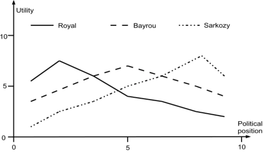
Figure 4 displays, for each candidate, the mean utility observed according to the self-reported position on the left/right axis. On average the utility functions are unimodal, symmetric around the mode and almost linear. Thus, the assumptions common to each model are reasonably satisfied.

Figure 4: mean utility as a function of political position

4.2

Estimation results

Table 2 presents the maximum likelihood estimates of the 5 SUR models described in the preceding sections. As already stated, Ur, Ub, Usare the utilities if Royal, Bayrou or Sarkozy

is elected. The constants bj for these three candidates are denoted by br, bb, bs respectively.

Similarly we define θr, θb, θs. Column [1] presents the maximum likelihood estimators of

the unconstrained system composed of the three equations. As already stated, there is no efficiency payoff to jointly estimate these equations if they are actually unrelated. The Breusch and Pagan (1980) statistic is 177.987, with 3 degrees of freedom.11 _{The 1 percent}

critical value is 11.34, so the hypothesis that the disturbances of the three equations are uncorrelated is rejected.

11

The Breusch-Pagan statistic is distributed as χ2

with M (M − 1)/2 degrees of freedom. In our appli-cation, M = 3, so this statistic has 3 degrees of freedom.

(15)

Table 2: Maximum likelihood estimates of the 5 seemingly unrelated regression models

[1] [2] [3] [4] [5]

N.C. Downs Additive Multiplicative Partisan valence valence valence br= bb= bs θr= θb= θs br= bb= bs br=_θK_r + C & & bb=Kθb+ C & θr= θb= θs bs=_θK_s + C Ur br 6.336*** 7.206*** 6.893*** 7.203*** (0.106) (0.053) (0.074) (0.053) 1 θr -0.475*** -0.652*** -0.656*** -0.658*** -0.480*** (0.028) (0.0143) (0.014) (0.020) (0.028) Ub bb 7.347*** 7.269*** (0.085) (0.061) 1 θb -0.683*** -0.640*** -0.669*** (0.025) (0.018) (0.018) Us bs 7.684*** 7.420*** (0.084) (0.071) 1 θs -0.734*** -0.654*** -0.740*** (0.019) (0.016) (0.019) K 5.154*** (0.417) C 3.873*** (0.275) Log-likelihood -17392.452 -17441.169 -17421.392 -17440.656 -17392.764 Likelihood ratio test 97.434*** 57.880*** 96.408*** 0.624 Notes: i.*, ** and *** represent 10, 5 and 1% significance, respectively.

ii. Standard errors are in parentheses.

iii. N.C. stands for no constraints, i.e. it provides the maximum likelihood estimates of the SUR model at unconstrained values of the parameters.

Columns [2]-[5] give the 4 constrained models discussed in the previous section. If restrictions on the utility functions of Column [1] are valid, then imposing them should not lead to a large reduction in the log-likelihood function. With the exception of the model which estimates the partisan valence utility function type (Model [5]), this is not the case.

Model [2] imposes the Downsian hypothesis, Ho : θj = θ and bj = b, ∀j. So, in our

application, estimating the Downsian utility type imposes 4 restrictions (θr = θb, θr = θs,

br = bb, br = bs). This model does not fit the data as well as the unconstrained model of

Column [1]. Indeed, the likelihood ratio test statistic is 97.434.12 _{The 1 per cent critical}

12

A likelihood ratio test is twice the difference between the log-likelihood functions of the unconstrained and constrained models (2 × (−17392.452 − (−17441.169)) = 97.434). It is asymptotically distributed as

(16)

value from the chi-squared distribution with 4 degrees of freedom is 13.28, so the hypothesis that the parameters in all three equations are equal is rejected. As a consequence, the Downsian utility type is not supported by the empirical evidence.

Model [3] is the SUR model where agents have additive valence utility type (Ho : θj = θ,

∀j). So there are 2 restrictions on Model [1] in our application (θr= θb, θr = θs). First, we

reject the null hypothesis that the additive valence utility type is valid: the likelihood ratio statistic, 57.88, is higher than 9.21, the 1 per cent critical value from the chi-squared table with 2 restrictions. So, similarly to the Downsian utility type, the additive valence utility type does not fit the data as well as the unrestricted model. Secondly, note that Models [2] and [3] are nested. In other words, Model [2] is not only a subset of the unrestricted model [1]: it is also obtained as a restriction on Model [3]. As a consequence, one might ask: do the additional parameters in the additive valence utility type model (compared to the Downsian) fit the dataset significantly better? The answer is yes. The likelihood ratio test is 39.55 and much higher than the 1 per cent critical value from the chi-squared distribution with 2 degrees of freedom (9.21 as already stated). So the relatively more complex additive valence utility type model is empirically more relevant than the simpler Downsian utility type model.

The SUR model where agents have a multiplicative valence utility type is presented in Column [4]. This model performs very poorly. On the one hand, the model with multiplicative valence utility type does not fit the data as well as the unconstrained model [1]: we reject the null hypothesis br = bb = bs from a likelihood ratio test (LRT = 96.41 and

p <0.000). On the other hand, the simpler Downsian utility type model fits the data as well as the multiplicative valence utility type model. Model [2] is a specification that is indeed a subset of Model [4]. The maximized value of the log-likelihoods of these two models are very similar (-17440.65 and -17441.16). The doubt cast on the empirical pertinence of the additional parameters in the multiplicative valence utility type (compared to the Downsian) is confirmed from a likelihood ratio test (LRT = 1.025 and p-value= 0.598).

Last but not least, Column [5] presents the maximum likelihood estimates of the par-tisan valence utility type model. The reduction in the log-likelihood function is very close to that of the unconstrained model. The likelihood ratio test is 0.62, which is far less than conventional critical values from the chi-squared distribution with one degree of freedom.13

imposing the restrictions.

13

There are 6 parameters in the unconstrained model (θ−1

(17)

Thus, this model is the unique constrained model that fits the data as well as the uncon-strained model of Column [1]. In other words, the partisan valence utility type is the only one that is supported by the empirical evidence.14

A clear cut result has emerged from the econometric analysis. A particular model, namely the partisan valence model, performs well in fitting our data. This fact calls for several comments. First, it supports the view that valence does matter to account for voters’ utility function since the Downsian model performs poorly. The multiplicative model per-forms particularly poorly, since the unrestricted multiplicative coefficients provide almost no efficiency gain. The picture is a bit better when we turn to the additive model - some efficiency gains are there. But this is not enough to conclude that it worth complicating the model by adding unrestricted additive parameters. The partisan model outperforms these models, but at the price of additional degrees of freedom.

Using the partisan valence model allows one to accurately estimate a valence index for each candidate. Note that these valence indices are estimated very precisely. Since this valence index differs across candidates, ranging from 0.48 to 0.74, the predictions of the partisan valence model are in sharp contrast with those of the Downsian model. In particular, such a difference in the valence indices predicts the victory of a candidate who is far away from the median. The winner of the election studied is located around 8 on a 0 to 10 scale measuring political position. According to the Downsian model such a candidate will loose against any candidate who is closer to the median position.

4.3

Robustness checks

To check the robustness of these results we repeated the regressions for various specifications and methods. These results are presented in the Tables in Appendix B.

First, note that the estimations in Table 2 assume that the utility functions are linear valence model (θ−1

r , θ −1

b , θ−1s , K, C), so there is one degree of freedom. The 10 per cent critical value from

the chi-squared distribution with 1 degree of freedom is 2.71.

14

Given that restricted and unrestricted parameters were simple to calculate in the models of Table 2, likelihood ratio tests to test the restrictions of the different models were convenient. But in complex models, the parameter vectors may be difficult to compute, particularly when nonlinear constraints are imposed, as in the partisan model. It will be the case in the last robustness check of the next subsection for reasons that will be clearly explained. A Wald test will be preferable even if this testing procedure is peculiar to the partisan valence model, as Appendix A explains; nevertheless, it provides similar results to a likelihood ratio test.

(18)

in distance, i.e. dij = |ai− xj|. This is far from being the only possible assumption.15 As

a consequence, the specifications in Table 1 consider that the distance is dij = |ai− xj|γ,

where γ is an exponent parameter, as do Poole and Rosenthal (1984, p.393). In other words, we have assumed that the utility of voter i if party j is elected is:

U(ai, xj, θj, bj) = −

1 θj

|xj − ai|γ+ bj + εij (12)

The models are now nonlinear systems with 3 couples of parameters {(br, θ−1r ), (bb, θ−1b ), (bs, θ−1s )}

as well as the coefficient γ to estimate. Two comments are in order. One can easily see that the estimated coefficient ˆγ is not significantly different from 1 in all the specifications.16

Thus, assuming that utility functions are linear in distance is supported by the empirical evidence. Furthermore, we show the likelihood ratio test for testing the restricted models at the bottom of each specification. Again, the unique theory that is not rejected by the data is the partisan valence theory.

We have also considered evidence relating to the model’s robustness to influential data, given that we would not have liked our results to be influenced by a few data points. To detect possible influential observations, we have computed studentized residuals after the estimation of the unconstrained model in Table 2. For each observation we have three equations {Uir, Uib, Uis}, so three residuals {ˆεir,εˆib,εˆis}, and three studentized residuals.

We have used various criteria to check if our results are robust. First, if one of the three studentized residuals is higher (in absolute value) than 3, this observation is excluded in all the 5 SUR models presented in Table 2. Five observations had at least one of their studentized residuals higher than 3.17 _{So the SUR models in Table 2 are estimated with 2455}

15

To name but a few examples, Alvarez and Nagler (1998, pp.64-65 and p.90) assume a spatial model of voting where the utility of voter i if the jth party wins the election is a function of the squared distance between the voter’s position and the party’s position. In their seminal paper, Poole and Rosenthal (1984, p.393) consider an exponent parameter on the distance, and propose specifications with various prespecified values of this parameter.

16

The z ratio for the test of the hypothesis that γ equals zero is 0.141¡≃ 1.007−1 0.052

¢

for the uncon-strained model, −0.109¡≃ 0_.995−1

0.049 ¢ for the Downsian one, 0.392 ¡≃ 1_.020−1

0.051 ¢ for the additive valence one,

−0.313¡≃ 0_.984−1

0.051 ¢ for the multiplicative one, and −0.040 ¡≃ 0_.998−1

0.049 ¢ for the partisan valence model. Thus,

the null hypothesis must not be rejected at the 1, 5 and 10 per cent significance levels.

17

Note that we have taken 3 as a first cutoff value because the highest studentized residual is 3.251. It concerns one residual of the Sarkozy equation in the unconstrained model of Table 2. The other two studentized residuals for this observation, those corresponding to the Royal and Bayrou equations, are 0.89 and 1.48. Three other observations have one of their studentized residuals that equals -3.247 (associated in the three cases with the Bayrou equation). The fifth one is a studentized residual that equals -3.146 (and

(19)

observations. Note that we have to be very concerned about studentized residuals higher than 3, but we can diminish this cutoff value. Table 3 presents estimation specifications where the cutoff value is 2.5. 71 additional observations are excluded in this Table, so the number of observations used to estimate the SUR models is 2384.18_{. Similar exercises were}

carried out using other criteria (not shown) and did not yield significantly different results from those of Table 2.19

Last but not least, we have been concerned by the fact that various respondents in the survey provided utility levels that are limit values (i.e. zero or ten). 375 respondents answered that they would have had a utility level Ur = 0 if Royal had won the election; 171

would have had Ub = 0 if Bayrou had won and 402 Us = 0 in a Sarkozy victory. Concerning

the other limit value, 245 respondents reported Ur = 10, 148 had Ub = 10 and 313 had

Us = 10. Our SUR models of Tables 2, 1, 2 and 3 might fail to account for the qualitative

difference between limit values and nonlimit values (strictly between zero and ten). To take account of this non-negligible proportion of respondents, we have estimated trivariate tobit models. There were, however, two difficulties.

There was a first practical difficulty to estimate such models because some observations are censored in the three equations of the models. The likelihood for these observations involves cumulative normal distribution of dimension three, which is a non-trivial problem.20

Fortunately, some progress has been made on the evaluation of higher than bivariate normal integrals. We have used the Roodman’s (2007) conditional mixed process estimator, CMP, a module available on the STATA software, to estimate the unconstrained model in Column [1] of Table 4.21 _{We were also able to estimate the Downsian, the additive valence and}

which is associated with the Bayrou equation again). There is no observation with the three studentized residuals higher than 3 at the same time.

18

2460 observations are used in Table 2. Five observations have at least one of their three studentized residuals higher than 3. 76 observations have at least one of their three studentized residuals higher than 2.5 (so 71 have at least one of their three studentized residuals between 2.5 and 3).

19

For instance, we have excluded observations which have at least two studentized residuals higher than 2.5 (7 observations are concerned) or higher than 2 (35 observations are concerned).

20

It concerns 111 observations: 9 respondents answered {Ur = 0, Ub = 0, Us = 0}, 50 answered {Ur =

0, Ub = 0, Us = 10}, 6 answered {Ur = 0, Ub = 10, Us = 0}, 33 answered {Ur = 10, Ub = 0, Us = 0}, 6

answered {Ur = 0, Ub = 10, Us= 10}, 2 answered {Ur= 10, Ub = 10, Us= 0}, 5 answered {Ur= 10, Ub=

10, Us= 10}. 21

CMP computes the trivariate normal cumulative density functions that are implied by such a model with the GHK (Geweke-Hajivassiliou-Keane) simulator. The estimates in Table 4 are obtained by this simulator, taking 200 draws per observation (for more details, see Cappellari and Jenkins 2006).

(20)

multiplicative valence models. Table 4 presents the results of all these models. We shows the likelihood ratio test for testing the restrictions implied by each model at the bottom of each specification. This testing procedure indicates that the Downsian, the additive valence and multiplicative valence are always significant, so the data reject these three theories.

The second problem concerns the partisan valence model. As already stated, the like-lihood ratio test requires calculation of both restricted and unrestricted estimators. The model becomes too cumbersome to estimate if the partisan valence restrictions are im-posed.22 _{As a consequence, a procedure similar to the one explained in Appendix A was}

carried out. A loop in the range 2.700 to 4.500, stepping by 0.001, was executed to obtain a Wald statistic for each of these values and to test the null hypothesis that at least one C in this range exists, such that the null hypothesis is true. Table 5 presents the results for some of these values. The Wald statistic is less than 4.61, the 10 per cent critical value from the chi-squared distribution with 2 degrees of freedom, when C ∈ [2.798; 3.985]. We obtain the lowest Wald test (2.178311) when C = 3.496. So the data do not reject the partisan valence theory.

5

Conclusion

So far, very few empirical papers have been devoted to valence issues, i.e. to non-policy factors. The present paper is a first step toward an empirical account of valence issues in elections. This paper has shown that traditional ways of introducing valence indices in utility functions, i.e. additively or multiplicatively, are too simple and perhaps misleading. Indeed, we have not found empirical evidence for these utility functions. In contrast, we have proposed a theoretically derived utility function with partisan valence that has strong empirical support. This strong empirical support is probably due to the fact that, contrary to the valence in additive and multiplicative models, the valence in the partisan valence utility function has a voter-specific dimension. All voters can indeed agree that a candidate has some objective characteristics (e.g., he is really willing to implement his campaign promises). However, this can affect voters in different ways. Thus, an objective characteristic does not necessarily result in a valence advantage, whereas existing models assume that a better valence index results in a greater utility for all voters. In the partisan model, a change along the valence dimension increases the utility of some voters but at the

22

(21)

same time decreases the utility of some other ones. All in all, a consensus on candidates’ characteristics leads to an increase in the political dissension among voters.

References

[1] Alvarez, R. Michael, and Jonathan Nagler. 1998. “When politics and models collide: Estimating models of multiparty elections.” American Journal of Political Science 42:55-96.

[2] Alvarez, R. Michael, and Jonathan Nagler. 2000. “A new approach for modelling strate-gic voting in multiparty elections.” British Journal of Political Science 30:57-75 [3] Ansolabehere, Stephen and James Snyder. 2000. “Valence politics and equilibrium in

spatial election models.” Public Choice 103:327-336.

[4] Aragones, Enriqueta, and Thomas R. Palfrey. 2002. “Mixed equilibrium in a Downsian model with a favored candidate.” Journal of Economic Theory 103:131-161.

[5] Ashworth, Scott, and Ethan Bueno de Mesquita (2005) “Valence competition and platform divergence.” Working paper, Princenton University.

[6] Breusch, Trevor S., and Adrian R. Pagan. 1980. “The Lagrange multiplier test and its applications to model specification in econometrics.” Review of Economic Studies 47:239-254.

[7] Burden, Barry. 2004. “Candidate positioning in US congressional elections.” British Journal of Political Science 34:211-227.

[8] Cappellari, Lorenzo and Stephen P. Jenkins. 2006. “Calculation of multivariate nor-mal probabilities by simulation, with applications to maximum simulated likelihood estimation.” Stata Journal 6:156–189.

[9] Carrillo, Juan D. and Micael Castanheira. 2002. ”Platform divergence, political effi-ciency and the median voter theorem.” CEPR discussion paper 3180.

[10] Carrillo, Juan D. and Micael Castanheira. 2008. “Information and strategic political polarization.” Economic Journal 118:845-874.

(22)

[11] Dix, Manfred and Rudy Santore. 2002. “Candidate ability and platform choice.” Eco-nomics Letters 76:189-194.

[12] Downs, Anthony. 1957. An Economic Theory of Democracy. New York: Harper and Row.

[13] Egan, Patrick. 2006. “Issue ownership and representation.” Working paper 2006-2, Institute of Governmental Studies.

[14] Erikson, Robert and Thomas R. Palfrey. 2000. “Equilibria in campaign spending games: Theory and data.” American Political Science Review 94:559-609.

[15] Greene, William. 2003. Econometric Analysis. Prentice Hall, 5th edition.

[16] Grose, Christian R. and Jason Husser. 2008. “The valence advantage of presidential persuasion: Do presidential candidates use oratory to persuade citizens to vote contrary to ideological preferences?” Mimeo.

[17] Groseclose, Tim. 2001. “A model of candidate location when one candidate has a valence advantage.” American Journal of Political Science 45:862-886.

[18] Herrera, Helios, David K. Levine and C´esar Martinelli. 2008. “Policy platforms, cam-paign spending and voter participation.” Journal of Public Economics 92:501-513. [19] Hollard, Guillaume, St´ephane Rossignol. 2008. “An alternative approach to valence

advantage in spatial competition.” Journal of Public Economic Theory 10:441-454. [20] Meirowitz, Adam. 2005. “Models of electoral contests.” Princeton University discussion

paper.

[21] Osborne, Martin J. 1995. “Spatial models of political competition under plurality rule: a survey of some explanations of the number of candidates and the position they take.” Canadian Journal of Economics 28:261-301.

[22] Poole, Keith T., and Howard Rosenthal. 1984. “US presidential elections 1968-1980: A spatial analysis.” American Journal of Political Science 28:282-312.

[23] Roodman, David M. 2007. “cmp: Stata module to implement conditional (recursive) mixed process estimator.” http://ideas.repec.org/c/boc/bocode/s456882.htm

(23)

[24] Sahuguet, Nicolas, and Nicola Persico. 2006. “Campaign spending regulation in a model of redistributive politics.” Economic Theory 28:95-124

[25] Schofield, Norman. 2003. “Valence competition in the spatial stochastic model.” Jour-nal of Theoretical Politics 15:371-383.

[26] Stokes, Donald E. 1963. “Spatial models of party competition.” American Political Science Review 57:368-377.

[27] Tanve, Morgane. 2008. “Do voters always prefer a favored candidate? The strategic use of imprecision.” Mimeo, University Paris 1 Panth´eon-Sorbonne.

[28] Wiseman, Alan E. 2005. “A Theory of partisan support and entry deterrence in elec-toral competition.” Journal of Theoretical Politics 18:123-158

[29] Zakharov, Alexei V. 2005. “Candidate location and endogenous Valence”, working paper EERC Moscow.

(24)

A

Appendix: An alternative approach to testing the partisan valence hy-pothesis

It is well-known that a shortcoming of the likelihood ratio test is that it requires estimation of both restricted and unrestricted parameter vectors. As far as both are simple to calculate, as in the models of Table 2, then a likelihood ratio test to test the restrictions is convenient. But in complex models, the parameter vectors may be much more difficult to compute, particularly when nonlinear constraints are imposed, as in the partisan model. It is the case in one robustness check of Subsection 4.3 where we estimate trivariate tobits. Given that a Wald statistic requires only the unrestricted parameter vectors, it will be preferable because it is much easier to compute. Furthermore, it is asymptotically equivalent to a likelihood ratio test. However, if one does a Wald test to test whether the restrictions of the partisan model are valid, it gives rise to a peculiar procedure.

To see that, let us assume that we want to test the partisan valence restrictions via a Wald test. The null hypothesis is H0 : bj = _θK

j + C ∀j = {r, b, s} ⇔ H0 : (br − C).θr =

(bb − C).θb = (bs− C).θs. Given that you do not have an estimated coefficient of C when

you only estimate the unrestricted model, you cannot compute the Wald statistic as such. You need to fix the coefficient C at one value, and then compute the corresponding Wald statistic. We have looped with C taking on values in the range 3 to 4.400, stepping by 0.001, to obtain a Wald statistic for each of these values. So we test if at least one C in this range exists, such that H0 is true. In other words, the null hypothesis becomes:

H0 : ∃C s.t. (br− C).θr = (bb− C).θb = (bs− C).θs

Table A1 presents the results for some of these values, testing this partisan valence restriction using the unrestricted parameters of Model [1] in Table 2. The Wald statistic has a chi-squared distribution and 2 degrees of freedom because C is no more a coefficient estimate. This is the peculiarity of this procedure: it does not give the same degrees of freedom as the likelihood ratio test. The 10 per cent critical value from the chi-squared distribution with 2 degrees of freedom is 4.61. At this conventional level, we cannot reject H0 as far as C ∈ [3.107; 4.345]. We obtain the lowest Wald statistic (0.7172343) when

(25)

Thus, we conclude that at least one C exists, such that the data do not reject our theory, and note that the C that minimizes the Wald test is very close to the estimated coefficient

ˆ

(26)

Table A1: Wald statistics under the null hypothesis that at least one C exists, such that the partisan valence hypothesis is true (using the parameter estimates of the unrestricted model in Column [1] of Table 2)

C 3.000 3.105 3.106 3.107 3.200 3.500 3.800 3.880 3.881 3.882 3.900 4.200 4.345 4.346 4.400

χ2₍₂₎ _5.351* _4.616* _4.608* _4.601 _3.949 _2.007 _0.792 _0.717 _0.717 _0.717 _0.721 _2.358 _4.596 _4.616* _5.762*

(p-value) ( 0.068) (0.099) (0.099) ( 0.100) (0.138) (0.366) (0.672) (0.698) (0.698) (0.698) (0.697) ( 0.634) (0.100) (0.098) (0.056) Notes: i. Observations: N = 2460.

ii.*, ** and *** represent 10, 5 and 1% significance, respectively.

iii. The Wald statistics are computed for the different values of C using the vector of parameter estimates of the unrestricted model in Column [1] of Table 2.

(27)

B

Appendix: Robustness checks

Table 1: Maximum likelihood estimates of the five seemingly unrelated regression models relaxing the hypothesis that utility functions are linear in distance

[1] [2] [3] [4] [5]

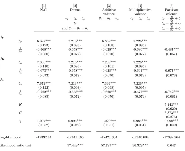
N.C. Downs Additive Multiplicative Partisan valence valence valence br= bb= bs θr= θb= θs br= bb= bs br=_θK_r + C & bb=θKb + C and θr= θb= θs bs=_θK_s + C Ur br 6.327*** 7.213*** 6.862*** 7.226*** (0.123) (0.093) (0.108) (0.095) 1 θr -0.468*** -0.658*** -0.628*** -0.680*** -0.481*** (0.060) (0.072) (0.070) (0.077) (0.057) Ub bb 7.336*** 7.213*** 7.238*** 7.226*** (0.110) (0.093) (0.101) (0.095) 1 θb -0.673*** -0.658*** -0.628*** -0.661*** -0.671*** (0.073) (0.072) (0.070) (0.073) (0.073) Us bs 7.672*** 7.213*** 7.394*** 7.226*** (0.122) (0.093) (0.098) (0.095) 1 θs -0.722*** -0.658*** -0.628*** -0.677*** -0.742*** (0.085) (0.072) (0.070) (0.079) (0.081) K 5.143*** (0.620) C 3.873*** (0.276) γ 1.007*** 0.995*** 1.020*** 0.984*** 0.998*** (0.052) (0.049) (0.051) (0.051) (0.049) Log-likelihood -17392.44 -17441.165 -17421.304 -17440.604 -17392.764 Likelihood ratio test 97.449*** 57.727*** 96.328*** 0.647 Notes: i. Observations: N = 2460.

ii.*, ** and *** represent 10, 5 and 1% significance, respectively. iii. Standard errors are in parentheses.

iv. N.C. stands for no constraints, i.e. it provides the maximum likelihood estimates of the SUR model at unconstrained values of the parameters.

(28)

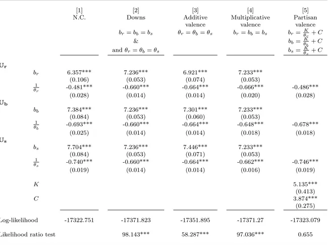
Table 2: Maximum likelihood estimates of the five seemingly unrelated regression models excluding observations with studentized residuals higher than 3 in absolute value

[1] [2] [3] [4] [5]

N.C. Downs Additive Multiplicative Partisan valence valence valence br= bb= bs θr= θb= θs br= bb= bs br= K_θ_r+ C & bb= K_θ_b+ C and θr= θb= θs bs= K_θ_s+ C Ur br 6.357*** 7.236*** 6.921*** 7.233*** (0.106) (0.053) (0.074) (0.053) 1 θr -0.481*** -0.660*** -0.664*** -0.666*** -0.486*** (0.028) (0.014) (0.014) (0.020) (0.028) Ub bb 7.384*** 7.236*** 7.301*** 7.233*** (0.084) (0.053) (0.060) (0.053) 1 θb -0.693*** -0.660*** -0.664*** -0.648*** -0.678*** (0.025) (0.014) (0.014) (0.018) (0.018) Us bs 7.704*** 7.236*** 7.446*** 7.233*** (0.084) (0.053) (0.071) (0.053) 1 θs -0.740*** -0.660*** -0.664*** -0.662*** -0.746*** (0.019) (0.014) (0.014) (0.016) (0.019) K 5.135*** (0.413) C 3.874*** (0.275) Log-likelihood -17322.751 -17371.823 -17351.895 -17371.27 -17323.079 Likelihood ratio test 98.143*** 58.287*** 97.036*** 0.655 Notes: i. Observations: N = 2455.

(29)

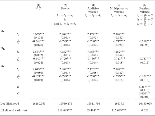
Table 3: Maximum likelihood estimates of the five seemingly unrelated regression models excluding observations with studentized residuals higher than 2.5 in absolute value

[1] [2] [3] [4] [5]

N.C. Downs Additive Multiplicative Partisan valence valence valence br= bb= bs θr= θb= θs br= bb= bs br= K_θ_r+ C & bb= K_θ_b+ C and θr= θb= θs bs= K_θ_s+ C Ur br 6.553*** 7.482*** 7.124*** 7.482*** (0.105) (0.051) (0.072) (0.052) 1 θr -0.549*** -0.729*** -0.736*** -0.747*** -0.550*** (0.028) (0.013) (0.014) (0.020) (0.028) Ub bb 7.564*** 7.482*** 7.553*** 7.482*** (0.082) (0.051) (0.059) (0.052) 1 θb -0.740*** -0.729*** -0.736*** -0.713*** -0.737*** (0.024) (0.013) (0.014) (0.018) (0.017) Us bs 8.013*** 7.482*** 7.726*** 7.482*** (0.080) (0.051) (0.068) (0.052) 1 θs -0.821*** -0.729*** -0.736*** -0.729*** -0.822*** (0.019) (0.013) (0.014) (0.015) (0.018) K 5.367*** (0.410) C 3.600*** (0.304) Log-likelihood -16480.053 -16539.475 -16511.795 -16537.9 -16480.065 Likelihood ratio test 118.843*** 63.484*** 115.693*** 0.023 Notes: i. Observations: N = 2384.

(30)

Table 4: Maximum likelihood estimates of the seemingly unrelated tobits

[1] [2] [3] [4]

N.C. Downs Additive Multiplicative valence valence br= bb= bs θr= θb= θs br= bb= bs & and θr= θb= θs Ur br 6.605*** 7.559*** 7.153*** 7.548*** (0.143) (0.075) (0.102) (0.075) 1 θr -0.609*** -0.791*** -0.792*** -0.805*** (0.039) (0.021) (0.021) (0.029) Ub bb 7.585*** 7.559*** 7.649*** 7.548*** (0.102) (0.075) (0.0801) (0.075) 1 θb -0.771*** -0.791*** -0.792*** -0.754*** (0.031) (0.021) (0.021) (0.025) Us bs 8.221*** 7.559*** 7.783*** 7.548*** (0.130) (0.075) (0.101) (0.075) 1 θs -0.928*** -0.791*** -0.792*** -0.811*** (0.033) (0.021) (0.021) (0.024) Log-likelihood -16423.305 -16462.512 -16445.488 -16458.431 Likelihood ratio test 78.414*** 44.366*** 70.252*** Notes: i. Observations: N = 2460.

(31)

Table 5: Wald statistics under the null hypothesis that at least one C exists, such that the partisan valence hypothesis is true (using the parameter estimates of the unrestricted model in Column [1] of Table 4)

C 2.700 2.796 2.797 2.798 2.800 3.100 3.400 3.495 3.496 3.497 3.500 3.800 3.985 3.986 4.000

χ2₍₂₎ _5.147* _4.611* _4.605* _4.600 _4.589 _3.117 _2.245 _2.178 _2.178 _2.178 _2.178 _3.026 _4.606 _4.617* _4.777*

(p-value) (0.076) (0.099) (0.099) (0.100) (0.100) (0.210) (0.325) (0.336) (0.336) (0.336) (0.336) (0.220) (0.100) (0.0993) (0.0991) Notes: i. Observations: N = 2460.

ii.*, ** and *** represent 10, 5 and 1% significance, respectively.

iii. The Wald statistics are computed for the different values of C using the vector of parameter estimates of the unrestricted model in Column [1] of Table 4.