Techno-economic analysis of PV/H2 systems

HAL Id: hal-01291900

https://hal.archives-ouvertes.fr/hal-01291900

HAL is a multi-disciplinary open access archive for the deposit and dissemination of sci-entific research documents, whether they are pub-lished or not. The documents may come from teaching and research institutions in France or abroad, or from public or private research centers.

L’archive ouverte pluridisciplinaire HAL, est destinée au dépôt et à la diffusion de documents scientifiques de niveau recherche, publiés ou non, émanant des établissements d’enseignement et de recherche français ou étrangers, des laboratoires publics ou privés.

Techno-economic analysis of PV/H2 systems

C Darras, G Bastien, M Muselli, P Poggi, B Champel, P Serre-Combe

To cite this version:

C Darras, G Bastien, M Muselli, P Poggi, B Champel, et al.. Techno-economic analysis of PV/H2 systems. International Journal of Hydrogen Energy, Elsevier, 2015, 40 (30), pp.9049-9060. �10.1016/j.ijhydene.2015.05.112�. �hal-01291900�

Techno-economical analysis of PV/H

system

C. Darras a,*, G. Bastien b, M. Muselli a, P. Poggi a, B. Champel c, P. Serre-Combe c

a

University of Corsica, UMR CNRS SPE 6134, Centre de Recherche Georges PERI, Route des Sanguinaires, 20000 Ajaccio, France

b

Ecole Centrale de Lille, Cité Scientifique, 59651 Villeneuve-d'Ascq, France

c

CEA LITEN, Antenne INES Corse, 17 rue des Martyrs, 38054 Grenoble, France

darras@univ-corse.fr, guillaume.bastien@centraliens-lille.org, marc.muselli@univ-corse.fr, philippe.poggi@univ-corse.fr, benedicte.champel@cea.fr, pierre.serre-combe@cea.fr

*

Corresponding author: Christophe DARRAS, email: darras@univ-corse.fr

Abstract

The purpose of this paper is to analyze the costs of PV/H2 systems connected to the grid and

sized to satisfy a power setpoint, using the ORIENTE® software. The aim is todetermine the optimal components’ size to minimize grid injection cost.

We study the case of guaranteed PV production, where the PV array is coupled to a hydrogen chain in order to be able to inject a constant power setpoint to the grid from 8am to 5pm (local time) all year long without failure (100 % level of satisfaction). Four power setpoints are studied: 100, 200, 300 and 400 kW.

The results show that regardless tothe power setpoint, the optimum system to be installed complies with the following ratios: installed PV power / power setpoint = 2.4-2.5, Electrolyzer nominal power / power setpoint = 0.72-0.75 and Fuel cell nominal power / power setpoint = 1. We have also found that the capacity of the H2 tanks corresponds to around 48-50days of autonomy

(number of days allowingonlythe fuel cells to fully supply the power setpoint).

1. Introduction

In times of global economical crisis, we will have to face one of the biggest technology shifts of the modern era. Indeed, in a world where energy demands continue to increase, the current generation means are problematic. Fossil fuels (main primary source [1]) pollute and are running out, affecting the health of the planet and its inhabitants [2, 3]. Concerning nuclear power, although not polluting during generation, it generates radioactive wastes that are difficult to manage, and the confidence in the nuclear sector is shrinking with each new disaster, such as recently in Fukushima. So it seems necessary to find other ways to produce energy we need.

Inexhaustible and non-polluting (during the production), renewable energy seems to be the ideal solution. However, there are still some problems to be solved such as intermittent generation, the fit between production and consumption [4], or cost due to their young technological [5]. The research community is working actively on resolving these problems.

The intermittence and the lack of adequacy between consumption and power production of renewable energies, limit their integration into the grids (30 % in France for example [6]), as it threatens their stability [7]. Storage is one of the solutions to settle these problems. That is why many studies have been conducted to see if it is technically and economically possible to store electrical energy from renewable energy sources [8-19].

J.K. Kaldellis et al. [8] haveconducted a techno-economic comparison of different means of energy storage (water pumping, compressed air, batteries, FC, ...) in insular conditions, on a real application: Greek Islands (Aegean Islands Archipelago). Due to the diversity in the sizes of these islands, different cases (from very small electrical networks to big island electrical networks) have been studied. These cases lead to different conclusions, but it appears from this study that with an existing electricity generation cost which is very expensive (due to the insular situation), renewable energies become profitable, and allow reducing the use of thermal power plants.

E.I. Zoulias et al. [9] haveconducted a techno-economical study with HOMER® [20] on Kythnos platform (8.8 kWp of PV array), by comparing a PV/diesel system and a PV/H2 system. They

concluded that the PV/H2 system will be profitable by 2020 (assuming a hypothetical reduction of H2

storage costs).

M. Rissanen et al. [5] have developed a software for sizing and estimating the cost of heat and electricity generation from PV/biogas/FC in a small office building (300 m²). They concluded that this technology is currently not competitive but different scenario consideredabout future costs can change that.

B. Shabani et al. [10] have sought to optimize by a techno-economical way, a PV/H2 plant

combined with heat recovery, with a program on Visual Pascal (Delphi). The simulation was tested under the conditions of Melbourne (Australia), with a load amounting 5 kWh/day. In addition to the significant gain in efficiency by recovering the heat generated by the FC, this optimization shows interesting results. The fuel cell in the system is conventionally sized to meet the peak of the load profile. However, an economic analysis illustrates that installing a larger fuel cell could lead to up to a 15 % reduction in the unit cost of the electricity to an average of just below 90 c€/kWh over the assessment period of 30 years. This result is explained by the fuel cell yield curve, which exhibits the highest efficiency at an intermediate operating point.

D.B. Nelson et al. [11] have developed a Matlab® program to design the components and optimize the cost of electricity produced by a wind turbine/PV/H2 system. This study was conducted at

a remote site: a house in the northeast Pacific. They then compared this system to a battery storage system, and found that the batteries were, at present, more profitable due to the performance of the FC.

Several papers have studied the complementarity of battery and H2 chain (see for example [12]

or [13]), and have shown that the combination of both storage means, coupled to an optimized strategy determining which storage technology to activate at each time is interesting from an economic point of view.

C. Budischaka et al. [14] have performed an optimization to minimize the total cost to power a large grid only from renewable energies, and see if it is technically and economically viable. The selected grid is PJM (Eastern U.S.), which represents one fifth of the United States (72 GW of

generation, with an average load of 31.5 GW). The calculations were performed for a period of four years. The program has tested 28 billion combinations, and it appears that on the one hand, it seems more interesting to oversize generation capacity (mostly wind) rather than using storage means and on the other hand, renewable energies will be cheaper than fossil fuels by 2030.

J. Andrews et al. [15] have conducted a dimensionless study (allowing easy adaptation to different situations) that gives an indicative evaluation of the economic viability of adding an hydrogen storage to a photovoltaic-based solar supply, either for a large-scale grid or small scale autonomous application. The study was applied to 78 big cities on five continents and in many different latitudes.It appears that the storage of H2 could be profitable in half of them (all of them if

prices fell). The places where H2 technologies are less profitable are the equatorial areas where the sun

is almost constant during the year.

In this context of research, we have investigated [21-23] the ability for hydrogen technologies coupled to renewable primary energy sources (PV, wind turbine,…) to smooth their fluctuating production and guarantee power injection level to the grid.

For that purpose, a software called ORIENTE® (Optimization of Renewable Intermittent Energies with Hydrogen for Autonomous Electrification, programmed with Matlab®) has been developed to model systems [21-24] coupling a PV array (solar panels and electric inverters) to a H2

chain (electrolyzer - H2, O2 and H2O tanks - and fuel cell). This software allows simulating the

operation of such systems, and optimizing their sizing and operating strategies based on technical considerations.

For the present study, we have developed an add-on to ORIENTE®. It allows performing a techno-economical analysis in order to assess the optimal sizes of PV/H2 system components and the

cost of electricity generation for a PV-guarantee application.

The operating of the PV/H2 system we study is to inject a constant power to the grid from 8am

to 5pm (local time) all year long without failure (100 % level of satisfaction: the power setpoint is always satisfied by the PV and or by the fuel cell, equivalent to LLP (loss of load probability) = 0 for a

non-connected system to the grid). Four power setpoints are studied: 100, 200, 300 and 400 kW. We assess the optimal size of the sub-systems in order to minimize the grid injection cost. The system is located to Ajaccio in Corsica island (France).

The paper is organized as follows. Section 2 details the contents of the techno-economical model. Then, Section 3 presentsthe parameters used for the simulations. Section 4 describes the results and their explanations. Finally, Section 5 concludes our study.

2. Techno-economical model description

We have developed a techno-economical optimization algorithm (Figure 1), using nested loops. The user defines a start and a final installed PV power, and for each value of this power, the program determines the most economical combination of other subsystems (inverters, electrolyzer, gas storage and fuel cell), which can supply the power setpoint. For this the user also defines the intervals and the steps in which the search is carried out to the size of the subsystems. Theses values are specified in Section 3.

Figure 1

2.1. Technical section

Concerning the technical part of the program, it consists in the calculation of the different flows (electric power, gas production and consumption,...). It is based on ORIENTE® which is described in previous paper [21-24]. In this part of the program, the system is divided in five subsystems: PV, inverters, electrolyzer, gas storage and fuel cell.

From meteorological data (Gi: solar irradiation and TA: ambient temperature; hourly time-step

on two years) and power setpoint (PPower_Setpoint: powerto send to grid), ORIENTE® calculates the flow

of power and gas using technical parameters of the different elements of the system.

The management (step (t) by step until tMax) of power flow of the simulation is as follows (see

 The PV production (PPV) supplies in priority the grid (PPower_Setpoint). In the case of an excess of

PV production (PExcess), of course taking into account the electrolyzer power threshold

(PThreshold_EL) and the electrolyzer nominal power (PNominal_EL), it creates H2 (ProdH2) via

electrolysis (PEL). The H2 quantity (QH2) is also checked to avoid exceeding the H2 tanks size

(QH2_Max). It is sometimes necessary to degrade the PV production to obtain the necessary

production. For this, the MPPT (Maximum power point tracking) inverters is used. It requires the inverters to operate at a lower efficiency.

 When the PV production is not able to satisfy the power setpoint (PMissing), the fuel cell (PFC)

supplies the complementary power. The fuel cell consumes for this H2 (ConsH2). If the missing

power is lower than the fuel cell power threshold (PThershold_FC), the PV production is

degrades.Thus the system is not faulty and the fuel cell is operating at its threshold. If the missing power is higher than the fuel cell nominal power (PNominal_FC), the system is faulty.

Figure 2

The size of the H2 tanks is not fixed. For against, the H2quantity at the start of the simulation is

fixed (QH2_Max = 10 9

Nm3). This value is used high threshold. To know the size of the H2 tanks

necessary to satisfy the power setpoint, simply subtract the value of this threshold with the H2 quantity

lowest during the simulation.

Each group of subsystem obtained during the optimization satisfies the power setpoint on 2

years. However, wheninstalled PV power is low, the system is not renewable. The H2 quantity early

and end of the 2 years is not the same (Figure 5). We will see again later that the optimum appears

from the moment where the system is renewable.

Threshold of the fuel cell and of the electrolyzer are fixed to 5 % of their respective nominal power (fixed during the optimization).The inverter efficiency curve as function of the inverter nominal power is represented Figure 3 (left abscissa). It is found that when inverters operate at more than 50% of their nominal power, efficiency is higher than 90%. The curve of production (electrolyzer) and

consumption (fuel cell) of H2 as function of respectively nominal power of the electrolyzer and the

fuel cell is represented Figure 3 (right abscissa).

Figure 3

2.2. Economical section

The economical model is based on the principle of net present value. The costs and revenues will be discounted and summed to obtain the net present value of the project [13]. The simulation method is the following: computation of the required sale price of electricity to achieve a net present value of zero for the lifetime of the project. This parameter is noted S€llPr and is calculated as follows: 𝑆€𝑙𝑙𝑃𝑟 𝑖 =− 𝐷𝑅𝑉 𝑖 8 𝑖=1 + 𝐶_𝐼𝑁𝑉 + 8𝑖=1𝐷𝐶_𝑅𝑒𝑝 𝑖 + 8𝑖=1𝐷𝐶_𝑂𝑀 𝑖 + 𝐷𝐶_𝑆𝑒𝑐 𝑃𝑟𝑜𝑑_𝑒𝑙𝑒𝑐 ∙ 𝐿𝑇𝑃 1+𝐼𝑅𝑒𝑙𝑒𝑐 _{1+𝐷𝑅 𝑗} 𝑗 𝑗 =1 (1)

Table 1 lists the economical parameters used in the equation 1.

Table 1

The system is divided into 8 subsystems: the land (i will be equal to 1 for this element and so on for the other subsystems), the photovoltaic array (i = 2), the inverters (i = 3), the electrolyzer (i = 4), gas storage (i = 5), the fuel cell (i = 6), infrastructure and manpower (i = 7) and finally the high voltage transformation post (i = 8).

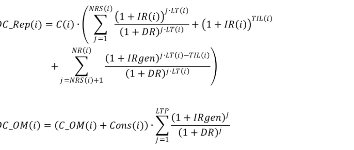
The three sums in the numerator of the equation (1) are calculated as follows:

𝐷𝑅𝑉 𝑖 = 𝐶(𝑖) ∙ 1 − 𝑁𝑅(𝑖) ∙𝐿𝑇(𝑖) 𝐿𝑇𝑃 ∙

1 + 𝐼𝑅(𝑖) 𝑇𝐼𝐿(𝑖)_{∙ 1 + 𝐼𝑅𝑔𝑒𝑛} 𝐿𝑇𝑃−𝑇𝐼𝐿(𝑖)

𝐷𝐶_𝑅𝑒𝑝(𝑖) = 𝐶 𝑖 ∙ 1 + 𝐼𝑅 𝑖 𝑗 ∙𝐿𝑇 𝑖 1 + 𝐷𝑅 𝑗 ∙𝐿𝑇 𝑖 𝑁𝑅𝑆 𝑖 𝑗 =1 + 1 + 𝐼𝑅 𝑖 𝑇𝐼𝐿 𝑖 + 1 + 𝐼𝑅𝑔𝑒𝑛 𝑗 ∙𝐿𝑇 𝑖 −𝑇𝐼𝐿 𝑖 1 + 𝐷𝑅 𝑗 ∙𝐿𝑇 𝑖 𝑁𝑅 𝑖 𝑗 =𝑁𝑅𝑆 𝑖 +1 (3) 𝐷𝐶_𝑂𝑀 𝑖 = 𝐶_𝑂𝑀(𝑖) + 𝐶𝑜𝑛𝑠(𝑖) ∙ 1 + 𝐼𝑅𝑔𝑒𝑛 𝑗 1 + 𝐷𝑅 𝑗 𝐿𝑇𝑃 𝑗 =1 (4)

For this, we need to determine the following six parameters (where int represents the integer part): 𝐶 𝑖 = 𝐶_𝑢𝑛𝑖𝑡(𝑖) ∙ 𝑁𝑢𝑚𝑏(𝑖) (5) 𝑁𝑅 𝑖 = 𝑖𝑛𝑡 𝐿𝑇𝑃 𝐿𝑇(𝑖) (6) 𝑇𝐼𝐿 𝑖 =𝑙𝑜𝑔 1 + 𝐼𝐿(𝑖) 𝑙𝑜𝑔 1 + 𝐼𝑅(𝑖) (7) 𝑁𝑅𝑆 𝑖 = 𝑖𝑛𝑡 𝑇𝐼𝐿(𝑖) 𝐿𝑇(𝑖) (8) 𝐶_𝑂𝑀(𝑖) = 𝐶 𝑖 ∙ 𝐶_𝑂𝑀_𝑢𝑛𝑖𝑡(𝑖) (9) 𝐶𝑜𝑛𝑠 𝑖 = 𝑁𝑢𝑚𝑏(𝑖) ∙ 𝐶𝑜𝑛𝑠_𝑒𝑙𝑒𝑐𝑡(𝑖) + 𝐶𝑜𝑛𝑠_𝑤𝑎𝑡(𝑖) (10)

Table 2 lists the economical parameters used in the equations 2 to 10.

Table 2

The two parameters in the numerator of the equation (1) are calculated as follows:

𝐶_𝐼𝑁𝑉 = 1 + 𝑖𝑛𝑠𝑡 ∙ 𝐶 𝑖

8 𝑖=1

𝐷𝐶_𝑆𝑒𝑐 = 𝐶𝑜𝑛𝑠𝐹 + 𝐶_𝐼𝑛𝑒𝑟𝑡 + 𝐶_𝑆𝑡𝑎𝑓𝑓_𝑡𝑟𝑎𝑖𝑛 + 𝐶_𝑇𝐺𝐴𝑃_𝑎𝑛𝑛 ∙ 1 + 𝐼𝑅𝑔𝑒𝑛 𝑗 1 + 𝐷𝑅 𝑗 𝐿𝑇𝑃

𝑗 =1

(12)

For this, we need to determine the following four parameters:

𝐶𝑜𝑛𝑠𝐹 = 𝐶𝑜𝑛𝑠𝐹_𝑒𝑙𝑒𝑐 + 𝐶𝑜𝑛𝑠𝐹_𝑊𝑎𝑡 (13)

𝐶_𝑖𝑛𝑒𝑟𝑡 = 𝐼𝑛𝑒𝑟𝑡 ∙ 𝑁𝑢𝑚𝑏(5) (14)

𝐶_𝑆𝑡𝑎𝑓𝑓_𝑡𝑟𝑎𝑖𝑛 = 𝑆𝑡𝑎𝑓𝑓_𝑡𝑟𝑎𝑖𝑛 ∙ 𝑁𝑢𝑚𝑏(2) (15)

𝐶_𝑇𝐺𝐴𝑃_𝑎𝑛𝑛 = 𝐶𝑜𝑒𝑓𝑓_𝑇𝐺𝐴𝑃 ∙ 𝑇𝐺𝐴𝑃_𝑎𝑛𝑛 (16)

Table 3 lists the economical parameters used in the equations 11 to 16. The model also takes into account the specific hydrogen safety requirement in France (see parameters highlighted in grey in this table) [25].

Table 3

The choice of the different parameters has been done by using recent years works [8-19, 25], and we have used the most representative values.

As our program aims at testing different combinations of parameters, it was necessary to define unit costs and to include links with the varying parameters.

The variables Prod_elecand Coeff_TGAP are respectively calculated in the technical part and according to the French regulation [25].

After having explained the theoretical background, we will now present the simulations performed.

3. Simulation parameters

In order to control more easily, for the grid manager, the balance between supply and demand, it is necessary for it to know the power that will be sent over the grid by the RES type power generation

(PV array, wind turbine,…). This will also increase the rate of integration of sources on the grid. In France, the solutions proposed by the CRE (French energy regulation commission) to resolve this problem are stipulated in the call for tender of the PV energy and the WT energy [26]. These solutions consist globally in coupling the renewable energies with a storage method and a meteorological data prediction method. The power sent by this system on the grid is also subject to certain constraint. For simple summary, these profiles must have a trapeze appearance, which is a power upslope, a tray with constant power, and finally a power downslope. The power producer must adhere to profile (whose power is bought by the grid Manager) on pain of financial penalty. For our study we will study four power setpoint profiles for which we will limit ourselves to the tray.

The annual power setpoint is as follows:

 From 8am to 5pm: constant at 100 kW (simulation 1), constant at 200 kW (simulation 2), constant at 300 kW (simulation 3), constant at 400 kW (simulation 4).

 From 0am to 8am & from 5pm to 12pm: constant at 0 kW.

Meteorological data were measured at the site of the MYRTE platform in Corsica. We used two years of data at one hourly time-step, and restricted the data to the daily period (8am to 5pm each day).This choice of restriction is due to the fact that we do not consider the phases of power upslope and power downslope in the profile to be sent tothe grid.

The intervals and the steps used in the techno-economical optimization algorithm are the following:

 PV: from 0 to 5 times the power setpoint by step of 10 kWp;

 Inverter: from 0 to 2 times the installed PV power by step of 10 kW;  Electrolyzer: from 0 to 2 times the installed inverter power by step of 5 kW;  Fuel cell:from 0 to 2 times the power setpoint by step of 25 kW.

Tables 4-a and 4-b show the values used in our economical model described above.

Table4-b

As can be seen in the table4, we assume a decrease in the investment cost of the PV, the inverters, the electrolyser, the Fuel Cell and the gas storage, due to the learning curve.

4. Results and discussion

Now, we have to observe and analyse the results obtained from our simulations.

Figure 4

Figure 4 shows, for the different power setpoints, the evolution of the required sale price of electricity to achieve a zero NPV, as a function of the ratio installed PV power / power setpoint. We separate the figure 4 into two parts, an overview (Figure 4 (A)) and zoom (Figure 4 (B)) on the most interesting part. The results are close whatever the power setpoint and the minimum sale price is obtained for a ratio between 2.4 and 2.5.

 When installed PV power is low (ratio < 2), the electrolyser rarely operates (for ratios lower than 1, there is even no electrolysis (see figure 6-a and 6-b) since it does no thave excess power). On the contrary, the fuel cell must constantly provide additional power to supply the setpoint. As a consequence, the required H2 gas tank size is huge and H2 content in the storage

decreases throughout the simulation (example Figure 5,‘__’). The cost for this sizing is very high.

 Increasing the installed PV power (up to 2.4-2.5 ratio) reduces the cost. Indeed, the PV power is large enough to supply the majority of setpoint and the electrolyzer (see figure 6-a and 6-b). The fuel cells is less operating which reduced the H2 gas tank size (example Figure 5, ‘---’).

 Beyond the 2.4-2.5 ratio, an increase of PV power only increases the cost. Indeed, much of the PV power is not used by the system (degraded power), it is limited by the inverter (see figure 6-a 6-and 6-b). It provides more power to the electrolyzer 6-and dem6-and less of the fuel cell, which has the effect of regularly cap gas tanks to their maximum (example Figure 5, ‘…’).

Figure 5 shows the H2 quantity evolution for the ratio 1, 2.5 and 4 of the simulation 1, as a

function of time. The behaviour of these curves is the same when the power setpoint is 100 kW, 200 kW, 300 kW or 400 kW.

 ‘__’: The H2 quantity steadily decreases, H2 is consumed but not produced.Indeed, the installed

PV power is equal to the power setpoint (ratio = 1) therefore in the best case the PV production is equal to the power setpoint, it is no H2 production (see figure 6-a and 6-b).

 ‘---’: The production and consumption of H2during the whole simulation are almost balanced.

The sizes of the PV, the inverter, the electrolyzer and the fuel cell are therefore adequatelysizedcompared to the power setpoint. The system is said to be renewable since there is as much H2 at the beginning and the end of the simulation.

 ‘…’: The H2tanks level is regularly atits maximum, which reduces the profitability of the

system (Figure 4). The H2 production is much greater than H2consumption, the size of tank is

limited, so it has a lot of H2 losses.

Figure 6-a

Figure 6-b

Figures 6-a and 6-b show the optimal sub-systems sizes (PV, inverter, electrolyzer and fuel cell), as a function of the ratio PV installed power / power setpoint. The behaviour of these curves is the same when the power of the setpoint are100 kW, 200 kW, 300 kW or 400 kW.

 When the ratio is less than 2, inverter size increases when increasing PV power. The electrolyzer power increases when the ratio is greater than 1, otherwise it is zero since there isnot PV production excess.

 When the ratio is greater than 2, the size of the inverter and the electrolyzer increases much less with increasing PV power. Is imposed as part of the optimization, a linear increase of the installed PV power. Nevertheless, technical-economic calculations limit the size of the inverter and the electrolyzer. Indeed, although the excess PV production increases, it is not economically viable to store it.

We can also see that the optimal power of the fuel cell is always equal to the power setpoint. Indeed a lower fuel cell power could generatea system failure (level of satisfaction inferior to 100%) in the absence of sunlight. The optimization doesnot choose fuel cell power greater than the power setpoint.The potential performance gain with greater fuel cell nominal power doesnot generate sufficient gain on storage (less consumption for the same power supply, therefore a smaller and cheaper tank).

Figure 7

Figure 7 shows, for the different power setpoints, the share of PV cost in the total cost, as a function of the ratio installed PV power / power setpoint. We separate the Figure 7 into two parts, an overview (Figure 7 (A)) and zoom (Figure 7 (B)) on the most interesting part. The results are close whatever the power setpoint.

The share of PV (include the inverters) in the total cost is logically 0 % when PV is not present (ratio zero) and reaches 24% for a 5-fold ratio. At the optimal PV size, this share is between 16% and 17%.

Figure 8

Figure 8 shows, for the different power setpoints, the share of H2 chain cost (include

electrolyzer, fuel cell and gas storage) in the total cost, as a function of the ratio installed PV power / power setpoint. We separate the figure 8 into two parts, an overview (Figure 8 (A)) and zoom (Figure 8 (B)) on the most interesting part. The results are close whatever the setpoint.

The share of H2 chain cost in the total cost is logically high (52 %) for low capacities of PV, and

decreases down to 10 % for a 5-fold PV/setpoint ratio, with a value between 25% and 26% for the optimal PV size.

Figure 9

Figure 9 shows, for the different power setpoints, the share of the remaining cost in the total cost (includeland, infrastructure and manpower), as a function of the ratio installed PV power / power

setpoint. We separate the figure 9 into two parts, an overview (Figure 9 (A)) and zoom (Figure 9 (A)) on the most interesting part. The results are close whatever the setpoint.

The share of the remaining cost in the total cost increases from 48 % when a zero PV/setpoint ratio to 67 % for a 5-fold ratio. At the optimal installation size, this share is between 56.5% and 58%.

Tabs. 5 and 6 summarize,for the different power setpoints, the optimization results of the system. Table5presents the optimal sizes of the subsystems and table6 gives the annual energies ratio and the system cost.

Table5

Table6

We can see in table 6, that whatever the power setpoint, the optimum system to be installed complies with the following ratios: installed PV power / power setpoint = 2.4-2.5,inverter power / power setpoint = 1.8-1.9 and electrolyzer nominal power / power setpoint = 0.72-0.75. We can also see that the fuel cells optimal power is equal to the power setpoint. Indeed the level of satisfaction being 100%, the electricity injected to the grid in non-sunny days must be full provided by the only fuel cells. One can note that the size of the converters is always lower than the PV power. A portion of the PV production is lost (degraded with MPPT inverters), but the system sizing is economically more interesting.This degraded PV power being quantified it will be used for a comparison in cost in Table 6 (cost without or with selling degraded PV production).Indeed, it normally sends on the grid only the power corresponding to the setpoint, however, it will look at the impact on the cost if the power was not degraded but sent surcharge on the grid.

We have also found that the capacity of the H2 tanks corresponds to around 48-50 days of

autonomy (number of days to allow the only fuel cells to fully supply the power setpoint profile).For example, for simulation 1, the fuel cell consumes 40 Nm3.h-1 to supply 100 kWh. If the fuel cell is working alone on the day (during 9 hours), it must provide 900 kWh, which requires 320 Nm3 of H2.

We can see in table 6, that whatever the power setpoint, around 77% of the energy is guaranteed by the PV and the remaining around 23% are supplied by the fuel cell. We also observed similar results in the distribution of PV production: 66-68% PV to power setpoint, 29-30% PV to electrolyzer and 1-3% degraded PV (not used). It is observed that the PV production is mainly used in the direct supplying of the power setpoint in order to limit the use of the H2 chain and losses. The cost without

selling degraded PV production ranges from 1.50 €/kWh to 1.60 €/kWh and ranges from 1.50 €/kWh to 1.56 €/kWh with selling degraded PV production. The sale of the degraded PV power reduces the cost of kWh around 2-4%.

…

5. Conclusion

…

6. References

[1] Renewable Energy Policy Network for the 21st Century (Ren21). 2011-Global Status Report. Available from: http://www.ren21.net/

[2] United Nations Environment Programme (UNEP). GEO-4 report. Available from: http://www.unep.org/

[3] Schlink U, Herbarth O, Richter M, Dorling S, Nunnari G, Cawley G, et al. Statistical models to assess the health effects and to forecast ground-level ozone. Environ Modell Softw 2006;21:547-58.

[4] Ahmed NA, Miyatake M, Al-Othman AK. Power fluctuations suppressions of stand-alone hybrid generation combining solar photovoltaic/wind turbine and fuel cell systems. Energy Conversion and Management, 2008;49:2711-9.

[5] Rissanen M, Schlabbach J, Strupeit L. Simulation for Technical and Economic Analysis of a Hybrid-Fuel-Cell System. POWERENG 2007, p. 353-58

[7] Molina MG, Mercado PE. Stabilization and control of tie-line power flow of microgrid including wind generation by distributed energy storage. Int J Hydrogen Energy 2010;35:5827-33.

[8] Kaldellis JK, Zafirakis D, Kavadias K. Techno economic comparison of energy storage systems for island autonomous electrical networks. Renew SustEnerg Rev 2009;13:378-92.

[9] Zoulias EI, Lymberopoulos N. Techno economic analysis of the integration of hydrogen energy technologies in renewable energy based stand-alone power systems. Renewable Energy 2007;32:680– 96.

[10] Shabani B, Andrews J, Watkins S. Energy and cost analysis of a solar hydrogen combined heat and power system for remote power supply using a computer simulation. Solar Energy 2010;84:144– 55.

[11] Nelson DB, Nehrir MH, Wang C. Unit sizing and cost analysis of stand-alone hybrid wind/PV/fuel cell power generation systems. Renewable Energy 2006;31:1641–56.

[12] Dufo-Lopez R, Bernal-Augustin JL, Contreras J. Optimization of control strategies for stand-alone renewable energy systems with hydrogen storage. Renewable Energy 2007;32:1102-26.

[13] Jallouli R, Krichen L. Sizing, techno-economic and generation management analysis of a stand alone photovoltaic power unit including storage devices. Energy 2012;40:196-209.

[14] Budischak C, Sewell D, Thomson H, Mach L, Veron DE, Kempton W. Cost-minimized combinations of wind power, solar power and electrochemical storage, powering the grid up to 99.9% of the time. J. Power Sources 2013;225:60-74.

[15] Andrews J, Shabani B. Dimensionless analysis of the global techno-economic feasibility of solar-hydrogen systems for constant year-round power supply. Int. J Hydrogen Energy 2012;37:6-18.

[16] Tzamalis G, Zoulias EI, Stamatakis E, Parissis OS, Stubos A, Lois E. Techno-economic analysis of RES & hydrogen technologies integration in remote island power system. Int. J Hydrogen Energy 2013;38:11646-54.

[17] Paola A, Fabrizio Z, Fabio O. Techno-economic optimisation of hydrogen production by PV e electrolysis: “RenHydrogen” simulation program. Int. J Hydrogen Energy 2011;36:1371-81.

[18] Bernal-Agustin JL, Dufo-Lopez R. Techno-economical optimization of the production of hydrogen from PV-Wind systems connected to the electrical grid. Renewable Energy 2010;35:747–58.

[19] Genç G, Celik M, SerdarGenç M. Cost analysis of wind-electrolyzer-fuel cell system for energy demand in Pınarbası-Kayseri. Int. J Hydrogen Energy 2012;37:12158-66.

[20] HOMER National Renewable Energy Laboratory (NREL), 617 Cole Boulevard, Golden, CO 80401-3393, URL: http://www.nrel.gov/homer

[21] Darras C, Modélisation de systèmes hybrides Photovoltaïque/Hydrogène: Applications site isolé, microréseau, et connexion au réseau électrique dans le cadre du projet PEPITE (ANR PAN-H), University of Corsica, PhDthesis 2010.

[22] Darras C, Muselli M, Poggi P, Voyant C, Hoguet JC, Montignac F. PV output power fluctuations smoothing: The MYRTE platform experience. Int. J Hydrogen Energy 2012;37:14015-25.

[23] Darras C, Sailler S, Thibault C, Muselli M, Poggi P, Hoguet JC, Melscoet S, Pinton E, Grehant S, Gailly, F, Turpin C, Astier S, Fontès G. Sizing of photovoltaic system coupled with hydrogen/oxygen storage based on the ORIENTE model. Int J HydrogenEnergy 2010;35:3322-32.

[24] Darras C, Muselli M, Poggi P, Logiciel ORIENTE, Dépôt UDC/CNRS sous le régime des droits d’auteurs de logiciel Propriété intellectuelle, Réf.: DL 04175e01 (2010).

[25] Dubois J, Hû G, Poggi P, Montignac F, Serre-Combe P, Muselli M, Hoguet JC, Vesy B, Verbecke F. Safety cost of a large scale hydrogen system for photovoltaic energy regulation. Int. J Hydrogen Energy 2013,38:8108-16.

[26] Available document via the link:

Figures and tables captions:

Figure 1 : Techno-economical optimization algorithm

Figure 2 : Simulation algorithm of power flow

Figure 3:

Left abscissa: Inverters efficiency curve as function of the inverter nominal power;

Right abscissa: Curve of production (electrolyzer) or consumption (fuel cell) d’H2 as function of

respectively the nominal power of the electrolyzer and the fuel cell

Figure 4: Required sale price of electricity (€/kWh) to achieve zero NPV, as a function of the ratio installed PV power / power setpoint;

− −: Area having the optimum point

Figure 5: H2 quantity evolution for the ratio 1, 2.5 and 4 of the simulation 1,as a function of time

Figure 6-a: Subsystems power sizing (Simulations 1 and 2), as a function of the ratio installed PVpower / power setpoint (part a);

− −: Optimum point

Figure 6-b: Subs-systems power sizing (Simulations 3 and 4), as a function of the ratio PV installed power / power setpoint (part b);

− −: Optimum point

Figure 7: Share of PV cost in the total cost, as a function of the ratio installed PV power / power setpoint;

− −: Area having the optimum point

Figure 8: Share of H2 chain cost in the total cost, as a function of the ratio installed PV power / power

setpoint;

Figure 9: Share of remaining cost in the total cost, as a function of the ratio installed PV power / power setpoint;

− −: Area having the optimum point

Table 1: Economical parameters quoted in equation 1

Table2: Economical parameters quoted in equations 2-10(U*: unit depends on i)

Table3: Economical parameters quoted in equations 11-16

Table 4-a: Economical parameters of our simulation (part a)

Table 4-b: Economical parameters of our simulation (part b)

Table 5: Optimal sizes of the subsystems according to the power setpoint