HAL Id: hal-01805163
https://hal.archives-ouvertes.fr/hal-01805163
Submitted on 17 Sep 2020
HAL is a multi-disciplinary open access
archive for the deposit and dissemination of
sci-entific research documents, whether they are
pub-lished or not. The documents may come from
teaching and research institutions in France or
abroad, or from public or private research centers.
L’archive ouverte pluridisciplinaire HAL, est
destinée au dépôt et à la diffusion de documents
scientifiques de niveau recherche, publiés ou non,
émanant des établissements d’enseignement et de
recherche français ou étrangers, des laboratoires
publics ou privés.
atmosphere-ocean-sea ice model compared to
proxy-based reconstructions
M. Blaschek, H. Renssen, Catherine Kissel, D. Thornalley
To cite this version:
M. Blaschek, H. Renssen, Catherine Kissel, D. Thornalley. Holocene North Atlantic Overturning
in an atmosphere-ocean-sea ice model compared to proxy-based reconstructions. Paleoceanography,
American Geophysical Union, 2015, 30 (11), pp.1503 - 1524. �10.1002/2015PA002828�. �hal-01805163�
Holocene North Atlantic Overturning in an
atmosphere-ocean-sea ice model compared to proxy-based
reconstructions
M. Blaschek1,2, H. Renssen1, C. Kissel3, and D. Thornalley4,5
1
Department of Earth Sciences, Faculty of Earth and Life Sciences, VU University Amsterdam, Amsterdam, Netherlands,
2Department of Meteorology and Geophysics, University of Vienna, Vienna, Austria,3Laboratoire des Sciences du Climat et de
l’Environnement/IPSL, CEA/CNRS/UVSQ, Gif-sur-Yvette, France,4Department of Geography, University College London, London, UK,5Department of Geology and Geophysics, Woods Hole Oceanographic Institution, Woods Hole, Massachusetts, USA
Abstract
Climate and ocean circulation in the North Atlantic region changed over the course of the Holocene, partly because of disintegrating ice sheets and partly because of an orbital-induced insolation trend. In the Nordic Seas, this impact was accompanied by a rather small, but significant, amount of Greenland ice sheet melting. We have employed the EMIC LOVECLIM and compared our model simulations with proxy-based reconstructions ofδ13C, sortable silt, and magnetic susceptibility (κ) used to infer changes in past ocean circulation over the last 9000 years. The various reconstructions exhibit different long-term evolutions suggesting changes in either the overturning of the Atlantic in total or of subcomponents of the ocean circulation, such as the overflow waters across the Greenland-Scotland ridge. Thus, the question arises whether these reconstructions are consistent with each other or not. A comparison with model results indicates thatδ13C, employed as an indicator of overturning, agrees well with the long-term evolution of the modeled Atlantic meridional overturning circulation (AMOC). The model results suggest that different long-term trends in subcomponents of the AMOC, such as Iceland-Scotland overflow water, are consistent with proxy-based reconstructions and allow some of the reconstructions to be reconciled with the modeled and reconstructed (fromδ13C) AMOC evolution. Wefind a weak early Holocene AMOC, which recovers by 7 kyr B.P. and shows a weak increasing trend of 88 ± 1 mSv/kyr toward present, with relatively low variability on centennial to millennial timescales.1. Introduction
The Atlantic meridional overturning circulation (AMOC) is critical to the global climate system. This circulation transports important amounts of heat (1.33 ± 0.4 PW at 26°N) [Johns et al., 2011] in the near-surface layer from the tropical Atlantic northwards to the midlatitude and high latitude of the Northern Hemisphere. In winter, part of this heat is released to the relatively cold atmosphere in the subpolar North Atlantic. This heat release results in relatively warm conditions over the greater North Atlantic region compared to similar latitudes of the North Pacific, with an air temperature increase of up to 10°C relative to the zonal mean climatology [Rahmstorf and Ganopolski, 1999], demonstrating the climatic importance of the AMOC.
There are two distinct driving mechanisms of the AMOC: the traditional thermohaline circulation and wind-driven upwelling [Kuhlbrodt et al., 2007]. On smaller scales a larger variety of processes including horizontal gyre circulation, local atmospheric cooling, and Greenland ice sheet melting play a role in driving its strength [Kuhlbrodt et al., 2007]. However, from Sandström’s [1908] theorem it is clear that surface buoyancy fluxes alone cannot supply the energy needed to sustain the AMOC [Kuhlbrodt et al., 2007]. Nonetheless, these surface fluxes are essential for deep-water formation [Huang, 2004] and thus the lower limb of the AMOC. If the density of a surface water mass is elevated to that of the underlying deep water masses, then a threshold density can be crossed and deep convection can occur. The deep mixing associated with this process leads to the formation of relatively dense deep waters, whichflow southward and sum up to form the North Atlantic Deep Water (NADW). In the present North Atlantic basin, deep convection occurs preferentially in the Labrador Sea, the Irminger Sea, and the Nordic Seas. The deep waters that form in the Nordic Seasflow southward at depth and have to cross a major sill, the Greenland-Scotland Ridge (GSR), to enter the North Atlantic Ocean as over-flow waters. These waters are known as Denmark Strait overover-flow water (DSOW) and Iceland-Scotland overover-flow water (ISOW), and are named after the two main locations of the overflow. The modern rates for DSOW and
Paleoceanography
RESEARCH ARTICLE
10.1002/2015PA002828 Key Points:
• δ13
C in the Norwegian Sea allows reconstructing convective activity • Paleomodeling allows reconciling
different trends in proxy-based reconstructions
• Long-term evolution of the AMOC is relatively stable since 7 kyr B.P.
Supporting Information: • Figure S1 Correspondence to: M. Blaschek, michael.blaschek@univie.ac.at Citation:
Blaschek, M., H. Renssen, C. Kissel, and D. Thornalley (2015), Holocene North Atlantic Overturning in an atmosphere-ocean-sea ice model compared to proxy-based reconstructions, Paleoceanography, 30, 1503–1524, doi:10.1002/2015PA002828.
Received 29 APR 2015 Accepted 19 SEP 2015
Accepted article online 30 OCT 2015 Published online 24 NOV 2015
©2015. American Geophysical Union. All Rights Reserved.
ISOW have been estimated at 2.2–3 sverdrop (Sv) (1 Sv = 1 × 10⁶m3s 1) and 2.4–3 Sv, respectively [Dickson and Brown, 1994; Hansen and Østerhus, 2000; Macrander et al., 2005; Smethie et al., 2013]. In addition, deep water formed in the Labrador Sea (so-called Labrador Sea Water, LSW) contributes 4–6 Sv to NADW [Schott et al., 2004]. Although deep convection has been observed in the Irminger Sea, quantified estimates of the contribu-tion to the NADW are not yet available [Kuhlbrodt et al., 2007]. Together with some entrainment of intermediate waters (about one third of the NADWflux) [Hansen and Østerhus, 2000], this adds up to a total southward NADW flux of 15–19 ± 2 Sv [Ganachaud and Wunsch, 2003; McCarthy et al., 2012; Smethie et al., 2013]. From this sum-mary, it is clear that changes in the rates of overflow waters or LSW formation will affect the strength of the NADWflow. A recent review by Lozier [2012] points out that from modern observations it is not clear whether the overturning strength in the North Atlantic can be directly linked to the intensity of deep-water formation. The biggest problem in this respect is undersampling. For example, the measurement period of the strength of the AMOC from a moored array across the North Atlantic at 26.5°N is relatively short (~7 yrs) [McCarthy et al., 2012], making its long-term evolution uncertain. However, modeling studies [e.g., Straneo, 2006; Rhein et al., 2011] have shown the impact of deep-water formation on the overturning circulation, such as Jungclaus et al. [2008], who found in a modeling study that 30% of the entire AMOC volume is directly coming from the Nordic Seas and that these waters together with considerable entrainment (approximately the same volume) form the backbone of the overturning. This discrepancy between modeled and observed results has not been resolved so far [Lozier, 2012]. However, considering longer timescales, numerous proxy-based recon-struction studies have attempted to extend these short present-day observations of AMOC strength into the past and to expand the knowledge of this so important climatic indicator.
1.1. Reconstruction of Past AMOC Changes
There are two categories of reconstructions of past North Atlantic Ocean circulation: surface and deep ocean reconstructions. This paper focuses on deep ocean circulation reconstructions, based on a number of proxies: ratios of carbon and oxygen isotopes (δ13C andδ18O) measured in shells of benthic foraminifera [Oppo et al., 2003; Kleiven et al., 2008; Hoogakker et al., 2011], deep ocean sediment characteristics, such as the sortable silt (SS) mean grain size [Bianchi and McCave, 1999; Hoogakker et al., 2011; Thornalley et al., 2013; Kissel et al., 2013], magnetic properties of grains (abbreviated as“κ”) [Kleiven et al., 2008; Kissel et al., 2009, 2013], geochemical data such as the Pa/Th ratio [McManus et al., 2004; Gherardi et al., 2009] and bulk mineralogy and isotopic composi-tion of sediments (such as Nd, Sm, and Pb) [Fagel and Mattielli, 2011]. In our present study, we focus on SS,κ, andδ13C, because thefirst two proxies focus on the speed of bottom water masses, which are thought to relate toflow speed in our model, whereas the third one focuses on the activity of ventilation and therefore supply of deep water, which is thought to relate to convective activity and the meridional overturning strength in our model. The combination of larger- and smaller-scale reconstructions in comparison with our model hopefully allows putting them into context and point toward biases and inconsistencies not to be discerned otherwise.
The SS proxy is based on the grain size of the terrigenous silt fraction from 10–63 μm, which can be used to reconstruct bottom current strength on the basis of depositional sorting associated with variableflow speeds [Praetorius et al., 2008]. Coarser-grain sizes indicate faster near-bottomflow speeds. The physical connection is based on Stokes’s settling principle, with numerous selective resuspension and deposition events resulting in a sorted deposit in which the grain size distribution reflects the mean kinetic energy of the flow, provided that eddy kinetic energy at the site is comparatively small [McCave et al., 1995, 2006; Praetorius et al., 2008]. Core locations have to be picked carefully to avoid problems. Uncertainty in the SS proxy may arise from potential source effects, spatial variability of theflow, downslope supply at continental margins, the influ-ence of ice-rafted detritus, and the inability to distinguish a high eddy kinetic energy from mean kinetic energy of theflow; however, these complications can largely be avoided by selecting suitable study sites and time intervals [McCave and Hall, 2006; Thornalley et al., 2013]. This method has been successfully applied to drift deposits, involving high sedimentation rates, from South of Iceland to reconstruct past rates of ISOW during the last glacial and present interglacial [McCave et al., 1995; Thornalley et al., 2013; Kissel et al., 2013].
The second proxy,κ, is the volume-normalized magnetic susceptibility measured on sediments in which titanomagnetites are the main magnetic carrier with uniform grain size. The transport of magnetic minerals from an identified source to the core location potentially allows the flow strength of bottom currents to be
deduced [Kissel et al., 2009]. This has been especially fruitful in determining the ISOW strength given a source of magnetic minerals at the Greenland-Scotland Ridge. The measurement ofκ is therefore an additional source of information complementary to SS. Uncertainties inκ are connected to the supply of magnetic source material and spatial variability of theflow [Kissel et al., 2013].
The third proxyδ13C is the ratio of stable isotopes13C and12C and is measured in the carbonate of benthic foraminifera shells (mostly Cibicidoides wuellerstorfi) and indicates the strength of deep ocean ventilation. During times of convection, surface waters that have higher values of carbon-13 compared to the deep ocean, sink and supply carbon-13 to the deep ocean. Hence, higherδ13C values in benthic foraminifera, which record the ambient deep oceanδ13C, are usually interpreted to indicate enhanced deep-water forma-tion and better ventilaforma-tion from the surface. Deep oceanδ13C values consequently depend on theδ13C value of the surface waters, whereas remineralization of organic carbon in the deep ocean acts as a source of error (0.1–0.3‰ present ocean) [Curry et al., 1988]. Surface δ13C in regions of deep convection is highly dependent on biological production and to a lesser degree on the air-sea gas exchange [e.g., Schmittner et al., 2013]. In the North Atlantic, deep waters have a different isotopic composition depending on the source region of the water masses. For example, Antarctic bottom water (AABW) is more depleted than NADW.
1.2. Holocene AMOC Changes
The long-term evolution of the AMOC is uncertain, and mostly only the evolution of its subcomponents, upper and lower limb or further subcomponents, such as the Florida Straitflow or the Greenland-Scotland Ridge overflow, is estimated by proxy-based reconstructions. For example, Thornalley et al. [2013] measured SS in drift deposits along a depth transect South of Iceland to reconstruct the ISOW strength over the past 9000 years. Their results show an early Holocene minimum followed by a maximum of ISOW at 7000 years before present (7 ka B.P.) and a subsequent decrease toward the present. Thornalley et al. [2013] subsequently compared these reconstructions to our modeling results discussed in Blaschek and Renssen [2013a] and found a good match between the reconstructed trend in ISOW strength and the simulated Nordic Seas winter convec-tion layer depth (CLD). However, convecconvec-tion or deep water mixing in the Nordic Seas can also be reconstructed fromδ13C. For instance, a reconstruction of Sarnthein et al. [2003] from a site near the western Barents Sea, shows little change in benthicδ13C of the deep ocean over the Holocene, indicating steady convection, without any long-term changes. This steady supply of deep waters, indicated byδ13C, within the Nordic Seas seems to be in conflict with an unsteady flow strength south of Iceland, indicated by SS. Consequently, at first sight, different proxy-based reconstructions suggest different trends in Holocene deep oceanflow. This raises the question if they are really in conflict or if they can be reconciled? Further investigation is thus required to better understand what these proxies represent and to analyze how the proxy-based reconstructions relate to model results. Afirst step, however, is to discuss previous, similar modeling studies on Holocene deep ocean circula-tion to see if these are consistent with the results of Blaschek and Renssen [2013a].
1.3. Palaeo-AMOC Modeling
Previous modeling studies have shown different trends in the simulated Holocene ocean circulation. Renssen et al. [2005] found a decreasing trend of deep convection in the Nordic Seas over the last 9000 years and an increasing trend in the Labrador Sea, hence stabilizing the strength of the AMOC by compensation. The deep convection decrease in the Nordic Seas was attributed to the expansion of Arctic sea ice as the climate was cooling toward the present, and more sea ice interfered with convective activity there. Renssen et al. [2005] explained the Labrador Sea increasing convection trend by a response to the orbitally forced surface cooling that enhanced surface density and as a compensation of the decrease in the Nordic Seas. However, they did not consider the impact of early Holocene ice sheet melting. A more recent study by Ritz et al. [2013] used a hindcast modeling approach to estimate the AMOC strength from surface proxy-based reconstructions, and then comparing these model results to231Pa/230Th ratios [McManus et al., 2004], indicative of deep water cir-culation strength, they found a weak decrease of the AMOC strength over the past 10,000 years, in agreement with the231Pa/230Th ratios. Incompatible to these previous studies, Lunt et al. [2006] employed an EMIC (GENIE-1) forced with transient ice sheet topography (ICE-5G) [Peltier, 2004] that showed an increase in AMOC strength over the last 10,000 years, interrupted by an abrupt event at about 9 ka B.P. These results are relatively similar to an accelerated transient simulation over the past 120 kyr that employed the FAMOUS GCM [Smith and Gregory, 2012], forced with different ice sheet topographies [Peltier, 2004;
Zweck and Huybrechts, 2005] and showed an increasing trend in AMOC strength for the past 10 kyr. Results indicated that the model and the subsequent AMOC strength responded strongly to the different ice sheet configurations. However, the impact of meltwater was not included in the study of Smith and Gregory [2012]. A 21 kyr long simulation (TraCE-21ka) employing CCSM3 and prescribed meltwater forcing shows a stepwise increase of the AMOC in the early Holocene much like the results from OGMELTICE in Blaschek and Renssen [2013a]; however, in the absence of meltwater forcing (after 7 kyr BP) the AMOC does not fully recover. In summary, different modeling studies that included different forcings (orbital parameters, Greenhouse gases, ice sheet topographies, and meltwater) indicate that the AMOC depends strongly on these forcings and on the model employed, mainly due to differences in model sensitivity. Hence, no consistent view on Holocene deep ocean circulation emerges from different proxy-based and model-based studies. Therefore, it is useful to examine this topic in more detail. We focus on the following questions: What are the contributions of different convection areas to overflow waters and to the simulated AMOC strength? To what extent are these model results for the AMOC consistent with proxy-based reconstructions? And finally, can we explain differences between proxies and model results, and uncover potential biases?
To address these questions, we provide a detailed analysis of the simulated AMOC dynamics within LOVECLIM and compare these simulations with selected proxy-based reconstructions.
In our present study, we focus on SS,κ, and δ13C, because thefirst two proxies focus on the speed of bottom-water masses, whereas the third one focuses on the activity of ventilation, therefore supply of deep bottom-water. Thus, these three proxies describe two characteristics of the overturning in the North Atlantic, the local, and the overall transport or circulation of water. We compare SS,κ, and δ13C reconstructions and their long-term evolution to our model simulations that cover the past 9 kyr. These simulations were performed with a fully coupled atmosphere-ocean-sea ice model of intermediate complexity by Blaschek and Renssen [2013a]. The Holocene started about 11.7 kyr B.P. and was dominated in its early phase by the decaying ice sheet remnants from the last glacial period until about 7 kyr B.P. [Blaschek and Renssen, 2013a]. During the past 7 kyrs, the Northern Hemisphere climate followed more or less the orbitally forced summer insolation trends [e.g., Kaufman et al., 2004; Kaplan and Wolfe, 2006; Lorenz et al., 2006] and were only slightly affected by trends in atmospheric greenhouse gas levels. Therefore, it is important to account for changes in ice sheets, orbital parameters, and greenhouse gases in our simulations. We designed four simulations including remnant ice sheet decay of the Laurentide ice sheet (LIS), described by meltwater and ice sheet topography on land, as well as melting of the Greenland ice sheet (GIS). The LIS is known to have released huge amounts of meltwater into the Labrador Sea and surroundings, preventing deep convection in the Labrador Sea until about 7 kyr B.P. [Hillaire-Marcel et al., 2001]. The melting of land-based ice sheets caused a prominent sea level rise of about 120 m (21 kyr B.P.) [Siddall et al., 2003], with about half of this rise (60 m) in the early Holocene (11.5 to 7 kyr B.P.). Lower sea levels and changed ocean dynamics such as shelfflooding [Blaschek and Renssen, 2013b], Bering Strait opening/closing [Hu et al., 2010], and tidal wave mixing [Schmittner et al., 2015] have impacts on the AMOC strength. However, given the timing of our simulations we consider these effects minor. The Bering Strait remains open, consistent with palaeoceanographic evidence indi-cating that this strait became active again at 11.1 kyr B.P. when sea level was 50 m below the current level [Elias et al., 1996].
In the following section we highlight important features of our model (section 2.1) and give detailed information on the experimental setup (section 2.2). In section 3 we introduce the results of our numerical simulations. In section 4.1 we present the proxy-based reconstructions and discuss the reconstruc-tions in the light of our modeling results in section 4.2.
2. Methods
2.1. Model
We performed our experiments with the Earth system model of intermediate complexity LOVECLIM (version 1.2) [Goosse et al., 2010]. We employed a version of this model that includes dynamical representa-tions of atmosphere, ocean and sea ice, land surfaces, and vegetation. Additional components, such as a dynamical ice sheet, the carbon cycle, or ice bergs, have not been activated in the present study. We present here a brief summary of the key components and refer to Goosse et al. [2010] for more details.
The ocean-sea ice component is CLIO3 [Goosse and Fichefet, 1999], consisting of a free-surface ocean general circulation model with a horizontal resolution of 3°x3° latitude-longitude and 20 vertical levels. Smaller scale processes not explicitly resolved by the model are parameterized. Vertical mixing and convection are para-meterized via an approximation of the turbulent kinetic energy, calculating viscosity and diffusivity, and an additional convective adjustment scheme, which increases vertical diffusivity in a statically unstable water column. To further improve the representation of dense waterflows, Campin and Goosse [1999] included a parameterization of downslope currents within the grid box resolution. These approximations for subgrid ocean processes require numerous parameters of which the isopycnal mixing is one of the most crucial [Stone, 2004]. The resolution of the model has implications on the amount of details being resolved by the bathymetry in the model compared to the real ocean. For example the Greenland-Scotland Ridge is uniformly about 1200 m deep compared to 400–800 m in the real ocean with canyons and trenches changing on scales far below what the model resolution does permit. The ocean model is coupled to a sea ice component [Fichefet and Maqueda, 1997, 1999] employing a three-layer dynamic-thermodynamic model. The atmo-spheric component is ECBILT [Opsteegh et al., 1998], a spectral T21, three-level quasi-geostrophic model coupled to a land-surface model that contains a bucket-type hydrological model for soil moisture and runoff. Cloud cover is prescribed according to observed present-day climatology [Rossow, 1996]. The dynamical vegetation model, VECODE [Brovkin et al., 2002], simulates two plant types (trees and grasses) and desert as a dummy type. In our simulations we prescribed the ice sheets manually.
LOVECLIM has been shown to have a climate sensitivity to a doubling of CO2concentrations just outside
the lower end (1.9K after 1000 years) [Goosse et al., 2010] as found in global climate models (2.1 to 4.5K) [Meehl et al., 2007]. Deep convection takes place in both the Nordic Seas and the Labrador Sea [Goosse et al., 2010], and the simulated deep ocean circulation is in good agreement with other model results [Weaver et al., 2012]. The model has been used successfully in numerous palaeoclimatological-modeling studies, for example, by Wiersma and Renssen [2006] to investigate the 8.2 kyr B.P. event and by Renssen et al. [2009, 2010, 2012] and Blaschek and Renssen [2013a, 2013b] in studies of the Holocene Thermal Maximum.
2.2. Experimental Setup
In this study we use the results of four transient experiments OG, OGMELT, OGMELTICE, and OGGIS that cover the last 9 kyr and have been discussed in detail by Blaschek and Renssen [2013a] and Thornalley et al. [2013]. All simulations have been forced with orbital parameters and atmospheric greenhouse gas concentrations in line with the PMIP3 protocol (http://pmip3.lsce.ipsl.fr). Initial conditions for each experiment are taken from quasi-equilibrium simulations at 9 kyr B.P. An overview of the forcings is provided in Figure 1.
Figure 1. Summary of forcings applied in different simulations. Blue line denotes changes in Laurentide Ice Sheet meltwater discharge in mSv. Green line shows Greenland Ice Sheets meltwater discharge in mSv. Red line denotes July insolation anomaly at 65°N compare to the present in Wm 2. Black line shows Greenhouse gases radiative forcing in Wm 2calculated using IPCC (2001) formulation.
We have performed one control simulation (OG) including only transi-ent orbital and greenhouse gases (present-day ice sheet topography) and two simulations including, additionally, either LIS meltwater (OGMELT) or the full LIS forcing (OGMELTICE). Following the setup of Renssen et al. [2009], the additional freshwaterflux was set to 0.09 Sv between 9 to 8.4 kyr B.P., decreas-ing slightly to 0.08 Sv between 8.4 and 7.8 kyr B.P. and droppdecreas-ing to 0.01 Sv between 7.8 and 6.8 kyr B.P. (Figure 1). These freshwater rates are based on adapted estimates of Licciardi et al. [1999] and do not include short-term drainage events like the one centered at 8.2 kyr BP [Alley and Ágústsdóttir, 2005], because the focus of our study is on multicentennial to millennial timescales. In OGMELTICE the effect of the disintegrating LIS was accounted for by changing the surface albedo and topography at 50 year time steps, interpolated from reconstructions provided by Peltier [2004], during the period 9 to 7 kyr B.P. Finally, we have performed a experiment (OGGIS) that included the GIS meltwaterflux, in addition to all forcings prescribed in OGMELTICE. As shown in Figure 1, this additional GIS meltwater was set to 13 mSv for 9 kyr B.P. and increases to 23 mSv from 9 to 8 kyr B.P. and then rapidly decreases to 3 mSv before vanishing completely at 7 kyr B.P. (estimates derived from Peltier [2004]). Considering the coarse model grid resolution (T21), early Holocene GIS topography changes in the model are relatively small [Blaschek and Renssen, 2013a] and are therefore neglected in this study.
3. Results From Transient Model Simulations
We propose to structure our results from the larger to the smaller scales in the following way: First, we will look at the Atlantic overturning strength in our simulations (section 3.1), which should compare well with δ13C in section 4.1.1, because both (hopefully) represent the overturning of water and are likely to be in good
agreement with each other (cf. section 4.2). Second, we will investigate the contribution of different convection areas to the overturning circulation (section 3.2), which will allow us to estimate the importance of these convection areas and make connections to the overflow waters as reconstructed by SS and κ at the Gardar Drift. Finally, we will investigate the exchange between the Nordic Seas and the Subpolar North Atlantic as well as the balance between NADW and AABW (section 3.3), which will be compared to SS-based reconstructions at the Orphan Knoll site andδ13C reconstructions in the eastern North Atlantic.
3.1. Atlantic Meridional Overturning Circulation
In our simulations, long-term changes of the AMOC strength are mainly driven by variations in the prescribed meltwaterflux. Our experimental setup with a considerable additional freshwater input related to the LIS and GIS melt from 9 to 7 kyr implies already that there is a difference between the early Holocene and the last 7000 years. We have to distinguish between simulations including only orbital parameters and greenhouse gases (OG), additional meltwater from the LIS (OGMELT), additional effects (albedo and topography changes on land) of the remnant LIS (OGMELTICE) and additional GIS melt (OGGIS), as summarized in Table 1. The simulated AMOC strength depends therefore on these choices and allows us to separate our analysis into an early Holocene (9 to 7 kyr), influenced by melting ice sheets and a later part (past 7 kyr), representing the transient climate change toward the present.
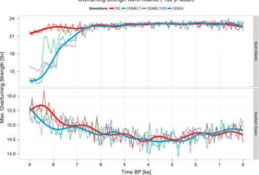
We present in Figure 2 the maximum overturning strength in the North Atlantic and the Southern Ocean, with the latter acting as a reference for interhemispherical changes. The strength in the North Atlantic follows the prescribed melt forcing in timing very precisely, indicating the rapid response due to meltwater from both the LIS and the GIS. However, we can see different reductions in OGMELT and OGMELTICE from 8.5 to 7 kyr B.P. originating from changes in the topography and albedo of the LIS, which modify the atmospheric circula-tion and the interaccircula-tion with the ocean. It has been previously reported [Renssen et al., 2009; Smith and Gregory, 2012] that the remnant ice sheet produced a downwind cooling effect on the North Atlantic, therefore cooling the surface ocean and allowing sea ice to expand in the whole Northern Hemisphere and especially in the Labrador Sea (as depicted for OGGIS compared to OG in Figure 3). In the Labrador Sea at 9 kyr B.P., the seaice area increases by 100 ± 10% in OGMELT, OGMELTICE, and OGGIS compared to OG (sea ice area 3.6 × 10¹¹m2)
Table 1. Summary of Experimental Setup
Name Forcings
OG Orbitals and Greenhouse Gases OGMELT OG + Laurentide Ice sheet meltwater (0.09– 0 Sv) OGMELTICE OGMELT + Laurentide Ice sheet topography + albedo OGGIS OGMELTICE + Greenland Ice sheet meltwater (0.025– 0 Sv)
and decreases for OGMELT earlier than for OGMELTICE. Some of the differences in AMOC strength (8.5–7 kyr B.P., Figure 2) between OGMELT and OGMELTICE are related to this change in sea ice extent. However, this effect is not always constant and evolves with the meltwater forcing and the decay of the land-based ice sheet. For example, in the beginning (i.e., at 9 kyr B,P.), simulation OGMELT shows a weaker AMOC strength (by 3 Sv) compared to OGMELTICE, because of the positive feedback the cooling effect of the remnant ice sheet in OGMELTICE has on the AMOC (i.e., strengthening, due to enhanced surface density). This has been attributed to a shift of convection from the Labrador Sea to the Irminger Sea by Renssen et al. [2009]. Likewise, as meltwater from the LIS decreases at 8.4 kyr B.P., the AMOC strength increases in OGMELT (+6.2 Sv) but remains lower in OGMELTICE (+0.6 Sv), because of the expansion of sea ice in the Labrador and the Nordic Seas. Hence, wefind that the combined forcing of meltwater and land-based ice sheet changes (topography and albedo) produce a stronger and less meltwater-dependent AMOC compared to melt-only forcing. However, including GIS melt in OGGIS reduces the AMOC between 9 and 8.5 kyr BP again, because of the relative closeness of the GIS meltwater
Figure 3. Deep convection areas in the North Atlantic in our model. Shown are 50 year averages of winter maximum convection depth in meters and maximum (red) and minimum (blue) sea ice extent for simulations OG and OGGIS at 9 kyr B.P. Convection areas are indicated by colored rectangles: Nordic Seas 45°W–30°E, 64–90°N (yellow), around Iceland 45°W–30°E, 50–64°N (green), and Labrador Sea 90–45°W, 50–70°N (blue).
15 18 21 24 14.0 14.5 15.0 15.5 16.0 North Atlantic Southern Ocean 0 1 2 3 4 5 6 7 8 9 Time BP [ka]
Max. Overturning Strength [Sv]
Simulations OG OGMELT OGMELTICE OGGIS
Overturning Strength North Atlantic ( 100 yr Mean)
Figure 2. Simulated Overturning in the North Atlantic and the Southern Ocean in sverdrop. Shown are 100 year averages of the maximum meridional stream function in the North Atlantic (45–75°N) and Southern Ocean (60–70°S) for four transient simulations. Thick lines indicate smoothed long-term trends for OG and OGGIS (n = 9).
to the convection area in the Irminger Sea. The additional GIS meltwater (13 mSv at 9kyr BP, Figure 1) sup-presses convection there. Therefore, we can see in the early Holocene a stepwise increase of the AMOC strength (OGGIS, 13.3 ± 0.5 (>8.5 kyr B.P.), 16.1 ± 0.5 (8.5–7.8 kyr BP), 20.1 ± 0.8 (7 kyr B.P.–the present)) related to the ice sheet forcing until it reaches present-day values at about 7 kyr B.P. (22.9 ± 0.6 Sv). The latter part shows a statis-tically significant increasing long-term trend (consistent with the long-term orbitally forced surface cooling, +88 ± 1 mSv/kyr), which is relatively weak compared to the much larger changes in the early Holocene. Consequently, we conclude that the early Holocene shows reduced AMOC strength, which comes to its full strength at about 7 kyr B.P., followed by relatively weak increase toward present. In the Southern Hemisphere the overturning circulation is hardly affected by the Northern Hemisphere meltwater and remnant ice sheet decay.
3.2. Convection Areas and Contribution to the Overall Deep Water Production
The strength of the overturning circulation (section 3.1) is associated with the intensity of deep convection at the different convection areas in the North Atlantic [Kuhlbrodt et al., 2007; Jungclaus et al., 2008]. Therefore, it is important to investigate convection areas and their contribution to the overall deep water circulation in the North Atlantic Ocean. We have three main deep convection areas in our model: the Labrador Sea, the Irminger Sea, and the Nordic Seas, as shown in Figure 3a for simulation OG. In the early Holocene, the melt-water from the LIS and GIS (simulation OGGIS, Figure 3b) reduces convective activity in these areas, especially convection in the Labrador Sea. Due to the drainage of ice sheet meltwater from both the LIS and GIS, con-vection in the Labrador Sea, the Irminger Sea, and the Nordic Seas are reduced in the early Holocene (Figure 4). In order to investigate this transient behavior, we calculated afirst-order estimate of the normal-ized convective volume (NCV), using the convection layer depth and grid box area for the three convection areas normalized against their sum (Figure 4), which should give an estimation of deep water production. Although not directly related, wefind that the changes in the overturning strength (Figure 2) agree well with the changes in NCV for the whole North Atlantic in the early part (Figure 4d, until 7 ka B.P.), giving lower values and a fast recovery. However, the long-term evolution in the second phase toward the present is reversed compared to overturning strength. Wefind a significant negative trend of 1634.6 ± 110 km3/kyr
0.16 0.20 0.24 0.28 0.05 0.10 0.15 0.20 0.25 0.50 0.55 0.60 0.65 0.8 0.9 1.0 1.1 Around Iceland Labrador Sea Nordic Seas
North Atlantic Region
9 8 7 6 5 4 3 2 1 0
Time BP [kyr]
Annual mean normalized potential convective volume [1] (100yr)
Simulations OG OGMELT OGMELTICE OGGIS
Contribution of major convection areas to North Atlantic convective volume
Figure 4. Estimated convection site contribution to the overall simulated deep convection in the North Atlantic for three convection areas (Labrador Sea, Around Iceland, and Norwegian Sea) and the sum of the three areas. Shown are 100 year averages of the maximum of the convective volume, which is calculated from convection layer depth (m) multiplied by the grid area (m2) and normalized by the sum of all convection areas. Boxes in Figure 3a indicate the areas.
(about 0.44%/kyr) in NCV in the Nordic Seas. The results show a substantial decrease of convection (and NCV as well), in the Nordic Seas (Figure 4c) in the early Holocene, thus potentially reducing the Greenland-Scotland overflow waters as well. It has been previously indicated by Thornalley et al. [2013] that reduced winter convection in the Nordic Seas (here represented by NCV in the Nordic Seas, Figure 4c) resemblesflow speed changes of the ISOW, resulting in less intense overflow before the major drop in ice sheet melt at 7 kyr B.P. The results support the idea that the strength of the overflow is linked to water mass properties, such as the density difference between the convected water and the surrounding waters. The question is if this link is also visible inflow speeds south of Iceland as recorded by SS.
3.3. The Subpolar North Atlantic
The subpolar North Atlantic is strongly affected by ice sheet melting during the early Holocene, resulting in a larger density difference with the Nordic Seas. We present the meridional velocities (negative is southwards) from two of our simulations (OG and OGGIS) at different depths. From the direction of theflow we can easily distinguish between what isflowing out of the Nordic Seas (below 1225 m) and what is flowing into it (above 850 m). These results are accompanied by varying density differences between the Nordic Seas and the subpo-lar North Atlantic at different depths. Before 7 kyr B.P. wefind a stronger inflow of lighter waters into the Nordic Seas (Figure 5), and a weaker outflow of denser waters from the Nordic Seas at greater depth (1225–1705 m) in our simulation including all ice sheet impacts (OGGIS) compared to OG. After 7 kyr B.P. there is hardly any dif-ference between the simulations and long-term trends do not significantly exist in both density-difference and flow speeds. The Nordic Seas are always denser (not explicitly shown, but indicated by the map in Figure 6) below 850 m in our model than the subpolar North Atlantic, and during the early Holocene the subpolar North Atlantic was more affected by the freshening than the Nordic Seas.
The density (Figure 6) of the 1225 m level in our model between OG and OGGIS shows that at this level the Arctic Ocean and the Nordic Seas are denser compared to the subpolar North Atlantic. The comparison shows Figure 5. Comparison of simulatedflow speeds south of Iceland and density differences between the Nordic Seas and the Subpolar North Atlantic from the four dimensional model outputs of our simulations OG and OGGIS. Shown are 50 year averages of the density difference (kg/m3) and the meridional velocity (mm/s), as well as smoothed lines (n = 9) to represent the long-term trends.
us that in OGGIS reduced convection, forced by melting ice sheets (meltwater and topography), affect the densityfield at this depth in the North Atlantic considerably, especially in the Labrador Sea and in the sub-polar North Atlantic. In addition, speed and direction of theflow are changed in OGGIS compared to OG, most noticeably south of the Denmark Strait, where overflow waters are directed toward the west. As expected, the density difference between the Nordic Seas and the subpolar North Atlantic results in strongerflow but only across the Denmark Strait and clearly not across the Iceland Scotland Ridge (ISR); otherwise, we would have found this in Figure 5b. To investigate this further we show in Figure 7 the deep waterflow across the Fram Strait, the Denmark Strait, and ISR. First, wefind only small changes in OGGIS compared to OG of deep water exchange between the Arctic and Nordic Seas, confirming that the Arctic Ocean is not a source or a sink of NS deep water. Second, wefind a stronger overflow in OGGIS compared to OG before 7 kyr B.P. in the Denmark Figure 6. Simulated exchange between the Nordic Seas and the Subpolar North Atlantic at 1225 m depth at 9 kyr B.P. Shown are 50 year averages of sea water density (kg/m3,filled contours) and water flow speeds (vectors) in the North Atlantic at the 1225 m depth level of our model for simulations OG and OGGIS.
Strait. ISOWflow is slightly reduced before 7 kyr B.P., followed by an increasing long-term trend toward present-day. Inconsistent with present-day observations, ISOW is much weaker than DSOW in our model. This difference is likely to arise from the simplification of the bathymetry in our model and from the fact that aflux is sensitive to the location in reality and in the model where it is measured, as it increases further away from the sill as more water is entrained. Nevertheless, the results indicate that in the early Holocene, the deep waterflow is redirected and increased toward the Denmark Strait. The early Holocene increase is potentially linked to lower densities in the western North Atlantic (Figure 6) compared to the eastern North Atlantic, therefore reinforcing theflow by a steeper density gradient.
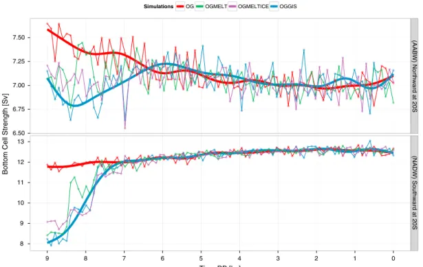
The combined deep water production of the North Atlantic results in an export of deep waters toward the Southern Hemisphere. At present the observed overflow waters across the GSR contribute about 40% (7.9 Sv) [Smethie et al., 2013] of the deep waters to the total NADW (19.6 ± 2 Sv) [Smethie et al., 2013]. In Figure 8 we show the strength of the bottom cell in the Atlantic at 20°S over the Holocene, representing either the northward AABW or the southward NADW. The export of NADW follows closely the maximum strength of the AMOC, which follows closely the prescribed meltwater forcing and gives a weak but steady increase toward the present. The AABWflow strength shows in general much less variations, and during the enhanced melting phase of the Northern Hemisphere ice sheets, a decreased northwardflow (up to 0.9 Sv in OGGIS compared to OG), in agreement with reduced export of NADW. However, the long-term trend of AABW in OGGIS seems to suggest a maximum at about 6 kyr B.P. with a continuous decrease toward the present ( 32 ± 1 mSv/kyr) as opposed to the long-term increasing trend in NADW (+60 ± 1 mSv/kyr). However, it should be noted that the changes in AABW strength are relatively small (within 1 Sv).
4. Discussion: Comparison to Proxy-Based Reconstructions
We would like to introduce the proxy-based reconstructions used in this studyfirst and describe in short what the corresponding authors have found and then continue with a discussion of our model results in context of these proxy-based reconstructions to answer our questions from the introduction: What are the contributions Figure 7. Modeledflow across the major pathways in the North Atlantic, the Fram Strait, the Denmark Strait, and the Iceland-Scotland Ridge. Shown are 100 year averages of bottom current strength in sverdrop for four simulations (OG, OGMELT, OGMELTICE, and OGGIS). Thick lines represent smoothed values (n = 9), and red bars indicate the standard deviation of simulation OG.
of different convection areas to overflow waters and to the simulated AMOC strength? And to what extent are these model results for the AMOC consistent with proxy-based reconstructions available? Can we explain differences between proxies and model results and potentially uncover biases?
4.1. Proxy-Based Reconstructions Over the Holocene
The large number of reconstruction studies that have been published over the past few years have improved our understanding of deep water circulation in the North Atlantic [Hoogakker et al., 2011; Kissel et al., 2013; Thornalley et al., 2013]. The combined interest is to extend the limited time period covered by observations of a major part of the climate system, the AMOC. In our study we focus on a set of SS-based reconstructions from Praetorius et al. [2008], Hoogakker et al. [2011], Kissel et al. [2013], and Thornalley et al. [2013], reconstruc-tions based on magnetic properties from Kissel et al. [2013] as well asδ13C from Sarnthein et al. [2003], Oppo et al. [2003], Kleiven et al. [2008], Praetorius et al. [2008], and Kissel et al. [2013] to compare to our model results over the past 9000 years. The locations are shown in Figure 9, and additional information on the exact locations is presented in Table 2, as well as information on the mean temporal resolution of the data. The time series are presented in Figure 10, grouped together by type (δ13C, SS,κ). For individual time series and other details we refer to the corresponding original papers and Figure S1 in the supporting information.
In the following we summarize key aspects of each reconstruction, as each location has some oceanographic factors that are relevant to its interpretation.
4.1.1. Iberian Margin
Shackelton et al. [2000] present aδ13C record measured in benthic foraminifera derived from a core from the Iberian margin (Figure 9, MD95-2042, 3146 m). Unfortunately, the Holocene part of this record was not studied in much detail in the presented study, because the focus of that study was on phase relation between Northern and Southern Hemispheres climate change. Their results show for the Holocene an early increase ofδ13C values until 7 kyr B.P., followed by a strong decrease until 5 kyr B.P., a subsequent recovery by 4.5 kyr B.P. and a weak decrease toward the present. The interpretation of these variations during the Holocene is likely to be similar to results from Oppo et al. [2003] (see below) that show a similar decrease at about 5 kyr B.P.
6.50 6.75 7.00 7.25 7.50 8 9 10 11 12 13 (AABW) Northward at 20S (NADW) Southward at 20S 0 1 2 3 4 5 6 7 8 9 Time BP [ka]
Bottom Cell Strength [Sv]
Simulations OG OGMELT OGMELTICE OGGIS
Export of deep water in the Atlantic ( 100 yr)
Figure 8. Export and import of deep waters in the North Atlantic in our model. Shown are 100 year averages of the maximum (minimum) of the meridional stream function of the bottom cell at 20°S in sverdrop indicating the northwardflow of AABW (max) and the southward flow of NADW (min). Thick lines show the smoothed long-term trends (n = 9) for simulations OG and OGGIS.
4.1.2. Western Continental Margin of the Barents Sea
Sarnthein et al. [2003] present aδ13C record from benthic foraminifera from the Western continental margin of the Barents Sea (GIK23258-2 at 1768 m depth), near the present-day Nordic Seas convection area. The interpretation of their results indicates that the AMOC during the Holocene was much more stable compared to glacial times, hence the relatively stableδ13C values of 1.21 ± 0.09‰.
Figure 9. Map of proxy core locations and schematic depiction of the bottom-current locations, relevant for this area.
Table 2. Summary of Proxy-Based Reconstruction Studies and Their Core Information as Displayed in Figure 9a
Core Investigator Parameter Location Depth Temporal Res.
Björn-Stack Thornalley et al. [2013] Mean SS Björn Drift 1200–2400 m 1000 years (bins) MD99-2251 Hoogakker et al. [2011] SS Björn Drift 2620 m 13 ± 4 years MD95-2024 Hoogakker et al. [2011] SS Orphan Knoll 3448m 50 ± 15 years ODP984 Praetorius et al. [2008] SS, Björn Drift 1648 m 766 ± 681 years
δ13C 379 ± 438 years
MD08-3182Cq Kissel et al. [2013] SS, CGFZ 3757 m 47 ± 90 years
Mag. Sus. 37 ± 66 years
∂13C 42 ± 23 years
MD03-2767Cq Kissel et al. [2013] Mag. Sus. Gardar Drift 2607 m 23 ± 8 years GIK23258-2 Sarnthein et al. [2003] δ13C W. Barent Shelf 1768m 60 ± 60 years ODP980 Oppo et al. [2003] δ13C Feni Drift 2179m 76 ± 49 years MD95-2042 Shackleton et al. [2000] δ13C Iberian Margin 3146m 708 ± 308 years MD03-2665 Kleiven et al. [2008] δ13C Eirik Drift 3440m 28 ± 17 years
4.1.3. Feni Drift
Oppo et al. [2003] published aδ13C record from benthic foraminifera from the ODP Site 980 at Feni Drift (Figure 9, ODP980, 2179 m). The record shows increasing values (1.2‰) until 7 kyr B.P., followed by long-term fluctuations with two minima at about 5 kyr and 2.8 kyr B.P. The location of this core allows it to monitor the influence of NADW versus southern originating waters, such as Lower Deep Water (LDW) or Antarctic Bottom Water (AABW), therefore showing times of enhanced or reduced NADW production. Olsen and Ninnemann [2010] emphasize that lowerδ13C values correspond better to NEADW rather than AABW at this site and relate variations inδ13C to changes in water mass distribution. Therefore, this site allows monitoring impacts Figure 10. Holocene proxy-based reconstructionsδ13C, magnetic susceptibility (κ), and sortable silt (SS) from the nine dif-ferent locations shown in Figure 9. (top)δ13C values for GIK23258-2 [Sarnthein et al., 2003], MD03-2665 [Kleiven et al., 2008], MD95-2042 [Shackleton et al., 2000], ODP980 [Oppo et al., 2003], and ODP984 [Praetorius et al., 2008]. (middle) Normalizedκ records for MD03-2676Cq and MD08-3182Cq [Kissel et al., 2013]. (bottom) Normalized SS records for Björn-stack [Thornalley et al., 2013], MD95-2024, and MD99-2251 [Hoogakker et al., 2011], and ODP984 [Oppo et al., 2003]. Thick lines denote smoothed splines (n = 9 or n = 13) to give longer-term trends. The normalized values are divided by their corresponding range. For absolute values we refer to the supplementary information.
from water masses with higherδ13C values, such as LSW, versus water masses with lowerδ13C values such as NEADW and in the most severe scenario AABW. Nevertheless, Oppo et al. [2003] conclude that strong variations (mostly a decrease) of NADW (at about 5 kyr B.P.) can occur without the interference of large ice sheets; there-fore, NADW seems to be more sensitive to larger changes than has been previously anticipated in interglacials.
4.1.4. Eirik Drift
Kleiven et al. [2008] present aδ13C record from benthic foraminifera from the Eirik Drift (MD03-2665, at 3440 m). The record allows monitoring properties of NADW along its western boundary flow path. The δ13C values are lower in the early Holocene, including a short event at about 8.3 kyr B.P. and continue to rise
until about 7 kyr B.P., when the present level of about 1‰ is reached. The core location is relatively deep and is at present influenced by DSOW and NADW.
4.1.5. Björn Drift
Praetorius et al. [2008] present the core of the Ocean Drilling Program Site 984 (Figure 9, ODP984, 1648 m), with reconstructions based on bothδ13C and sortable silt. The sortable silt record is included in the Björn-Stack [Thornalley et al., 2013]; however, we highlight that this record is important because both proxies are available from the same core. The location allows reconstructing ISOW at a certain depth. The authorsfind that during the Holocene, variations in the current strength (SS) are observed without corresponding varia-tions in the source water (δ13C). For example the record shows a rise ofδ13C from 10 to 5 kyr B.P., a subse-quent drop until 3 kyr B.P. followed by higher values again by 1 kyr B.P. The corresponding SS record shows hardly any variations but a weak long-term increasing trend. This indicates thatδ13C values are not always associated with changes in the current strength; thus, according to these authors, it is important to pair both proxies for an integrated view of the dynamics of the overturning circulation [Praetorius et al., 2008].
4.1.6. Orphan Knoll and Gardar Drift
Hoogakker et al. [2011] present two high-resolution sortable silt records from the Gardar Drift (2620 m) and the Orphan Knoll (3448 m; Figure 9, named MD99-2251 and MD95-2024) sites. Theflow speeds near the Gardar Drift site are likely to represent changes in the ISOW at a certain depth and give a long-term decreasing trend toward the present. Kissel et al. [2013] have raised some doubts about the reliability of the results from MD99-2251, due to influences from the piston coring process. Flow speeds at the Orphan Knoll represent the deepest North Atlantic water mass and describe the characteristics of a kind offinal NADW mass, after ISOW, DSOW, and LSW have been incorporated. Still, there are potentially more water masses that can influence flow speeds at that location such as the Lower Deep Water (LDW), Antarctic Bottom Water (AABW) and Subpolar Mode Water (SPMW). The long-term trend at the Orphan Knoll is weak but increasing over the past 10,000 years.
4.1.7. Charlie-Gibbs Fracture Zone (CGFZ) and Gardar Drift
Kissel et al. [2013] introduce a new and updated (compared to Kissel et al. [2009]) reconstruction based on magnetic property records at the Gardar Drift (2607 m) and at the CGFZ (3757 m), where the ISOWflow west-wards. The core at the Gardar Drift is in close proximity of Hoogakker et al. [2011] core MD99-2251, allowing a close comparison between SS and the reconstructedκ. The second core lies further south at the CGFZ, pro-viding sortable silt,κ, and δ13C. The combination of all three proxies from one core is a good anchor in the comparison toward each other. The record at the Gardar Drift, representing ISOW current strength, shows higher values in the early Holocene, with a minimum at 8.2 kyr B.P., followed by a new maximum at 6.5 kyr B.P. and a subsequent decrease toward the present. The second core further south shows similar trends in magnetic properties but reconstructed values of SS differ especially in the earliest part of the Holocene. Theδ13C values are lower in the early Holocene and remain relatively constant after 7 kyr B.P. The core near the CGFZ is likely to show not only ISOW influences but some impacts from other water masses such as LDW as well [McCartney, 1992; LeBel et al., 2008; Kissel et al., 2013]. The polynomialfit is different between the original paper (n = 5) and the data presented here (n = 13).
4.1.8. South Iceland Rise and Björn Drift
Thornalley et al. [2013] introduce a new reconstruction based on sortable silt from multiple cores at different depth along the main axis of the ISOW over the past 9000 years (Figure 9, named by us as Björn-stack). In total 13 cores (in a depth range of 1200–2300 m, including the Praetorius et al. [2008] data) have been used to reconstruct the strength of the ISOW. The multicore setup allows the reconstruction to account for the ver-tical migration of the main axis of the ISOW. The authors have shown that their reconstructed overflow strength from SS corresponds well with winter convection layer depth in the Nordic Seas modeled by Blaschek and Renssen [2013a], employing the very same model as this study. The concept behind this is that denser waters, as indicated by a deeper mixed layer depth, will overflow faster across the ISR and will be
recorded by SS after the sill. The SS-based reconstruction reveals a maximum ISOW strength at 7 kyr B.P. with a subsequent decrease toward the present.
We conclude that in all records, some impacts have been found that relate to their specific location and can influence the reconstructed values on different timescales. However, what these impacts are and how these have evolved over time, is uncertain. Our interest in the present study is on long-term trends, such as millen-nial changes in the AMOC strength. When we compareδ13C and SS records in Figure 10, we can see that some long-term trends agree with our simulation results and some disagree. We propose to look at the three proxies separatelyfirst before we continue with the combined discussion in section 4.2.
4.1.9. Carbon-13 Records
From 10 to 7 kyr B.P. theδ13C records of the various locations share relatively low values compared to the lat-ter inlat-terval (from 7 kyr B.P. toward the present) and a similar upward trend between 8 and 7 kyr B.P. These overall common features inδ13C originate from numerous feedbacks such as vegetation cover, a cooler and saltier ocean, ocean circulation, and changes in the calcification budget of the ocean on glacial to inter-glacial timescales [Broecker and Peng, 1986; Köhler et al., 2005; Jansen et al., 2007]. Lower values are in general found during glacial times, rising to higher values during interglacials. After 7 kyr B.P. the cores to the eastern North Atlantic (MD95-2042, ODP980) show lower values and higher variability compared to the one core near the western Barent Sea margin, in the Norwegian Sea. This difference has been discussed by Hoogakker et al. [2011], and they propose that this difference emerges due to an increase of LDW volume (lowδ13C values originating from AABW) during the early Holocene, and the onset of deep eastward advection of LSW as Labrador Sea convection started at about 7 kyr B.P. [Hillaire-Marcel et al., 2001]. Oppo et al. [2003] interpreted δ13Cfluctuations on millennial timescales in core ODP980 as an indicator of northern versus southern deep
water influence, arguing as well that a strong reduction in δ13C must be the result of mixing with a depleted δ13C water mass such as LDW originating from AABW. Oppo et al. [2003] have argued that it is likely that these
variations inδ13C are originating from a southern source rather than a northern source. However, Olsen and Ninnemann [2010] attribute these changes to variations in LSW versus NEADW contribution, thus putting the origin of the signal in the North Atlantic. In the Norwegian Sea (GIK23258-2) the reconstructedδ13C values are relatively constant for the rest of the Holocene, with minor variations, thus suggesting that a continuous sup-ply of deep water must have reached the site. The core MD08-3183Cq near the CGFZ shows overall lower values in the early Holocene, particularly at about 8.8 kyr B.P., followed by relative constant values from 7 kyr B.P. toward the present. The low values were interpreted by the authors as changes in the mixing of LDW and ISOW. The offset of this event compared to the other reconstructions may indicate depth migration with time [Kissel et al., 2013].
In summary, theδ13C records from different locations in the North Atlantic show early Holocene lower values and an increase between 8 and 7 kyr B.P. and from 7 kyr B.P. onward higher variability in the subpolar North Atlantic compared to the Nordic Seas. This indicates weaker vertical mixing or convective activity in the early phase and steady and strong activity toward the present, with impacts from LSW versus NEADW contribution at core locations south of Iceland and with influences from AABW at the core locations in the deep northeast Atlantic impacting the recorded signal there. The early Holocene phase is, however, potentially impacted by the glacial to interglacial differences and not only by changes in the ocean circulation.
4.1.10. Sortable Silt Records
The long-term trends in the SS-based reconstructions from different sites do not exhibit a common trend, but some of the reconstructions agree with each other. Therefore, we have to make a distinction based on their location. In our comparison, four out of five sites are from the area south of Iceland at the Gardar Drift (MD99-2251, ODP984, and Björn-stack) and at CGFZ (MD03-3182Cq) and one is from the Orphan Knoll site near the Labrador Sea (MD95-2024). The latter one is thus representing a“downstream” water mass, including ISOW, DSOW, LDW, and LSW. Four of the SS-based reconstructions are created from a single core and one uses multiple cores at different depth (Björn-stack). The advantage of a multicore reconstruction is that a potential migration of the mainflow can be considered and an overall strength can be calculated by stacking all the records [Thornalley et al., 2013]. Thornalley et al. [2013] have reported that the core of the ISOW was shallower (~1400 m) in the early Holocene, deepest at about 5 kyr B.P. (~2200 m) and again becoming shallower (~1800 m) toward the present. This suggests that the interpretation of long-term trends in a single core should consider its depth and position. In Figure 10 we present normalized SS records (divided by their range) that are comparable to each other. Regardless of their actual position, wefind that there are different long-term trends
in all reconstructions. The Björn-stack shows weaker values in the early Holocene followed by a maximum around 7 kyr B.P. and a decrease toward the present. The Labrador Sea core (MD95-2024) gives a weak but variable increase toward the present. MD99-2251 gives a steady but variable decrease toward the present, similar to the decrease in MD08-3182Cq from 8 kyr BP toward the present, and ODP984 exhibits hardly any long-term trend. Despite the relatively coarse temporal resolution (~1000 year) of the Björn-stack, the long-term decrease after 7 kyr B.P. agrees with a decrease in MD99-2251 and MD08-3182Cq, but before 7 kyr B.P. only MD08-3182Cq and the Björn-stack agree.
4.1.11. Magnetic Susceptibility Records
The two reconstructions from a core at the Gardar Drift (MD03-2676Cq) and a core near the CGFZ (MD08-3182Cq) show remarkably similar long-term evolutions (Figure 10). Both records show an early Holocene decrease with a local minimum at about 8.5 kyr B.P. followed by an intermediate maximum between 7 and 6 kyr B.P. and a subsequent decrease toward the present. The core at the Gardar Drift is in close proximity to the SS record of core MD99-2251 and indicates similar variability and long-term trends. The Björn-stack SS record agrees even closer to theκ from MD03-2676Cq from 8.5 kyr B.P. toward the present, thus supporting the reconstruction of deep waterflow from both proxies, SS, and κ.
In summary, the strength of the deep ocean circulation during the Holocene is not clear from all the recon-structions we looked at. Most of theδ13C records seem to agree to some extent that the overturning strength increased from the early Holocene to the present, whereas the sortable silt records South of Iceland seem to show that the ISOW strength decreased over the Holocene and the strength of deep waterflow increased in the Labrador Sea over the Holocene. Theκ-based reconstruction agrees relatively well with some of the SS-based reconstructions, supporting the early Holocene decrease, a maximum at about 7–6 kyr B.P. and the long-term decrease in ISOW strength. The question is if and how these results can be actually reconciled. Our model results might be helpful to answer this question.
4.2. Discussion: Comparison of Model Results and Proxy-Based Reconstructions
The goal of this study is to get a better understanding of Holocene changes of the North Atlantic Ocean circulation and compare model results to reconstructions from proxies. We have introduced reconstructions based on δ13C, SS, and κ records from the subpolar North Atlantic and the Nordic Seas in section 4.1 (Figure 10) and have shown results from four transient model simulations in section 3. In this section we discuss modeled and reconstructed deep water circulation.
4.2.1. Carbon Isotopes
From theδ13C-based reconstructions we might conclude that there is an early part, where all records presented give lower values, followed by increasing values until about 7 kyr B.P., when different signals start to emerge. In ourfirst attempt we compare these reconstructions with the stream function of the AMOC to represent the volume transport on a large scale. Indeed, there are some similarities, a relatively weak early part followed by a relatively stable part, with higher values until the present. However, cores MD95-2042 (Iberian Margin) and ODP980 (Feni Drift), which are located in the eastern North Atlantic, seem to show much higher variability within the last 7000 years than the core in the Norwegian Sea (GIK23258-2). It has been argued by the authors of these reconstruction studies that theδ13C values are likely to have been affected by the supply of LDW, originating from AABW, which is particularly low in carbon isotopes. This is potentially also visible in the overall lowerδ13C values from core MD08-3182Cq (3757m), which shows a strong minimum at 8.8 kyr B.P. and some variations at 5 and 4 kyr B.P., similar to cores in the eastern North Atlantic. Thus, strong variations inδ13C could indicate the balance between LDW and ISOW, and as we showed in Figure 8 the strength of the simulated AABWflux shows some small changes (0.9 Sv) and gives a maximum at around 6 kyr B.P. Our model results seem to indicate such variability inδ13C induced by the supply of deep waters from the Southern Hemisphere. Therefore, a site that is not influenced by these impacts from the Southern Hemisphere could correspond better to the strength of the AMOC in our model. For this, we could use core GIK23258-8 from the shelf of the Western Barent Sea. Indeed, there seems to be a better correspondence between simulated AMOC strength (as in Figure 2a) andδ13C of the benthic foraminifera from this core. The question remains, however, why the magnitude of the early decrease in AMOC strength is not that well recorded at this site, as changes in the modeled AMOC strength are stronger and would suggest stronger impacts inδ13C as well. However, from our analysis of the convection areas (Figure 3), it has become clear that the NS site is not shut down, but its ventilation depth is reduced in the early Holocene (Figure 4c), which is
potentially still sufficient to supply enough13C to the bottom. Therefore, changes that are to be recorded inδ13C have to affect the supply of deep waters or the magnitude of changes to the overall AMOC strength is underes-timated. However, the long-term downward trend in convective volume from NS is as well not recorded in GIK23258-8, because the signal is probably too weak to show up in this ventilation proxy. We cannot rule out that an increasing trend in atmosphericδ13Catm[Schmitt et al., 2012], levels a decreasing trend inδ13C in the ocean.
Variations inδ13C in the deep subpolar NA are likely to be influenced by AABW supply, but it cannot be said with certainty from a comparison to our model results. Changes in the total solar irradiance (TSI) or volcanic eruptions or other potentially unknown changes are not included in our simulations, which might be responsible for stronger variations in these proxies [Oppo et al., 2003; Praetorius et al., 2008] or the AMOC strength.
4.2.2. Sortable Silt
The SS-based reconstructions at different core locations in the subpolar North Atlantic, give different long-term trends that are influenced by their location and their depth. For the reconstructions near the Gardar Drift (MD99-2251, ODP984, and Björn-stack) wefind that the long-term trends vary substantially between the reconstructions. It has been noted by Thornalley et al. [2013] that single-core reconstructions have a potential weakness, as the position of the mainflow axis can migrate with depth, potentially creating a signal that is not necessarily related to changes inflow speed. Regardless, long-term trends in SS do not compare well with the evolution of the AMOC strength in our model (Figure 2), with a weak opposing trend of +88 ± 1 mSv/kyr (OGGIS) from 7 kyr B.P. to the present. However, the simulated changes in mixed layer depth or convective volume in the NS (Figure 4c) show a significant decrease toward the present (NCV 1634.6 ± 110 km3/kyr, about 0.44%/kyr),which corresponds better to the reconstructed SS-based over-flow evolution at the Gardar Drift from the Björn-stack. The greater decrease in the proxy compared to the convection volume decrease suggests that convection volume might not be a direct proxy for the ISOW. The corresponding decrease, nevertheless, suggests that a link between deep water production, its water mass properties and the recorded SS South of Iceland exists. Therefore, when convection is shallower, less dense waters are produced and exported via the ISR and result in less deep waterflow, leading to a maximum of SS that is recorded in a shallower core. The ISOW is influenced not only by the actual depth of convection in the NS but also by the density structure of the subpolar North Atlantic [Thornalley et al., 2013], which will influence how deep overflowing waters will sink and mix. Thus, it is important to know what the density difference between the subpolar North Atlantic and the Nordic Seas was during the Holocene. Our analysis shows that the density difference (Figure 5) increased before 7 kyr B.P. in a simulation including remnant ice sheet meltwaters (OGGIS) compared to a simulation including only orbital and greenhouse gases (OG). From Figure 6 it is clear that the density in OGGIS decreased compared to OG all over the North Atlantic at that depth and most likely in the whole water column as well due to ice sheet melting. During this early phase, the potential for overflow waters was actually increased and in Figure 7, we find that the modeled DSOW strength is increased, whereas the ISOW strength is decreased. Our model shows higher DSOW strength at the present compared to recent observations [Smethie et al., 2013], which might indicate an unsuited comparison of reconstructed and modeled deep waterflow strength at a site influenced by either DSOW or ISOW. A potential source of this bias could be the simplified bathymetry in the model. However, the origin of these waters is undeniably the NS convection site and changes will be exported either via the Denmark Strait or the ISR. Thornalley et al. [2013] used this argumentation already and more information from the same model does not help to explain these reconstructions better. The relatively low resolution of our model does not allow looking at depth changes along the main axis of the ISOW. The stronger decrease of ISOW strength compared to a modest decrease in convection depth or volume might be the effect of additional factors, likely including changes in the partitioning of ISOW and DSOW which contribute to a stronger decrease at the Gardar Drift site. A recent publication [Moffa-Sanchez et al., 2015] found such an antiphased relationship between ISOW and DSOW over the past 3000 years. Nevertheless, wefind that simulated lower flow speeds at the Gardar Drift site (Figure 5b) agree with lower SS-basedflow estimates in the early part before 7 kyr B.P., but modeled long-term trends do not correspond to trends seen in either mean SS or modeled NS convection depth. Considering all our results presented in this study, we cannotfind a consistent explanation for the long-term decreasing trend of SS in MD99-2251 at the Gardar Drift, especially as values at about 9.4 kyr B.P. are highest. It has been noted by Kissel et al. [2013] that this core might have some perturbation due to the coring process itself, implying that the results may be less reliable. Some of the SS-based reconstructions have a higher variability compared to theδ13C-based records as well as some other SS records, partly because of a higher temporal resolution (Table 2). However, the long-term increasing trend in MD95-2024 in the Labrador Sea is
consistent with the simulated trend in Labrador Sea convective volume (Figure 4b). The location of the core and its depth (3448 m) would also suggest that there might be a link to the NADWflow (Figure 8b) and its strength over the Holocene. Indeed, weak long-term increasing trends can be found in both simulated NADW strength and SS-basedflow speed in the second phase (after 7 kyr B.P.), in contrast to the early phase. Nevertheless, this similarity is rather small.
4.2.3. Magnetic Susceptibility
Reconstructions from the Gardar Drift and the CGFZ indicate similar long-term trends and correspond well with SS-based reconstructions from the Gardar Drift, indicating a close relationship to ISOW. Given this similarity,κ values correspond as well with NS convection depth (Figure 5b), showing an early Holocene low (8.8–8 kyr B.P.), followed by a maximum (7–6 kyr B.P.) and a subsequent decrease toward present.
4.2.4. Final Considerations
At this point it is unclear whether the mismatch between modeled AMOC strength and reconstructed deep water flow can be attributed to localized effects that are important for the proxy signals, but cannot be resolved by the model, or to a more fundamental problem in the model and its deep water production,flow and overturning. Considering that we employed this model, we think it is appropriate to conclude with a discussion of our model’s performance and emphasize the need for higher resolution models to conduct long-term experi-ments including several different forcings. In a present-day comparison of CMIP5 and EMIC models [Weaver et al., 2012], LOVECLIM produces a maximum of the AMOCflow (23.2 Sv) that is somewhat higher than the majority of the models, while the decrease of the AMOC strength to future warming is comparable to most models used in that study. Unfortunately, there are hardly any comparisons of deep waterflow including multiple models, as well as palaeoclimate-modeling studies discussing past deep water circulation changes in details during the Holocene [besides Thornalley et al., 2013]. From present-day observations [Smethie et al., 2013] we know that our model shows weaker ISOW and stronger DSOW and that a comparison to reconstructions depending only on one of these components alone might be impacted by this specific bias. However, we have to emphasize that the agreement between the ISOW strength recorded from SS in the Gardar-stack and the convective volume in the NS is still valid, as the source signal is likely to be transported to the location of the reconstruction.
5. Conclusions
We have compared four transient simulations over the past 9000 years including early Holocene remnant ice sheet decay to proxy-based reconstructions usingδ13C,κ, and SS in the North Atlantic. We have in detail tried to reconcile the different long-term trends in the reconstructions with the help of our model results, to gain a bet-ter understanding of the AMOC changes of the past 9000 years. In summary our results indicate the following: 1. Althoughδ13C can be affected by numerous processes, benthicδ13C in the Norwegian Sea may
poten-tially provide some information on convective activity in the Norwegian Sea. However, it is likely that only large changes in the supply of deep water can alter the recorded d13C signal, such that the proxy is rather insensitive to Holocene changes in deep convection.
2. δ13C in the deep subpolar North Atlantic is influenced by13C-depleted waters originating from AABW, leading to low values at North Atlantic sites. Our investigation partly supports the idea that long-term variations seen inδ13C values are likely to be caused by the influence of AABW in the deep North Atlantic. However, the corresponding variations in AABW advances and retreats are weak in the model and give therefore only an indication of these dynamics.
3. Wefind a good agreement between depth-weighted SS and κ at the Gardar Drift with simulated Nordic Seas normalized convective volume, suggesting a direct link between ISOW and NS convection activity. The combined results suggest weaker ISOW at 9 kyr B.P., followed by a maximum at about 7–6 kyr B.P. and a subsequent decrease toward the present. However, the proxy-based decrease in ISOW is greater than that seen in modeled normalized convective volume or convection depth, because of additional factors, likely including changes in the partitioning of ISOW and DSOW which contribute to a more pronounced decrease in ISOWflow strength, compared to a modest decrease in convection depth. 4. Inconsistent with present-day observations, our model shows stronger DSOW compared to ISOW.
Considering this imbalance a model bias that remains constant over time and our simulation including LIS and GIS forcings (OGGIS) compared to an orbital and GHG simulation (OG), we find in the early