HAL Id: hal-00700245
https://hal-brgm.archives-ouvertes.fr/hal-00700245
Submitted on 26 Oct 2012HAL is a multi-disciplinary open access archive for the deposit and dissemination of sci-entific research documents, whether they are pub-lished or not. The documents may come from teaching and research institutions in France or abroad, or from public or private research centers.
L’archive ouverte pluridisciplinaire HAL, est destinée au dépôt et à la diffusion de documents scientifiques de niveau recherche, publiés ou non, émanant des établissements d’enseignement et de recherche français ou étrangers, des laboratoires publics ou privés.
A set of Eurocode 8-compatible synthetic time-series as
input to dynamic analysis
Aurore Laurendeau, Mathieu Causse, Philippe Guéguen, Mathieu Perrault,
Luis Fabian Bonilla, John Douglas
To cite this version:
Aurore Laurendeau, Mathieu Causse, Philippe Guéguen, Mathieu Perrault, Luis Fabian Bonilla, et al.. A set of Eurocode 8-compatible synthetic time-series as input to dynamic analysis. 15th World Conference on Earthquake Engineering : 15th WCEE, Sep 2012, Lisbon, Portugal. in press, 10 p. �hal-00700245�
A set of Eurocode 8-compatible synthetic time-series
as input to dynamic analysis.
A. Laurendeau, M. Causse, P. Guéguen & M. Perrault ISTerre, CNRS, Université Joseph Fourier, IFFSTAR, Grenoble, France
L.F. Bonilla
IFSTTAR, Paris, France J. Douglas
BRGM, Orléans, France
SUMMARY:
Non-linear dynamic analysis of existing or planned structures often requires the use of accelerograms that match a target design spectrum. Here, our main concern is to generate a set of motions with a good level of fit to the Eurocode 8 (EC8) design spectra for France. Synthetic time series are generated by means of a non-stationary stochastic method. To calibrate the distributions of various strong-motion parameters, we first select a reference set of accelerograms for a type B site category from the PEER Ground-Motion Database, which are then adjusted to the target spectrum through wavelet addition. Finally, we analyse non-linear seismic responses of a soil column including pore pressure effects and ductile structures using these records, revealing considerable variability despite the similarities in terms of spectral acceleration.
Keywords: Eurocode 8(EC8), spectrum-compatible time-histories, nonlinear site response, structural response
1. INTRODUCTION
The selection of accelerograms for earthquake engineering (both the geotechnical and the structural branches) is becoming increasingly important with the growing use of nonlinear dynamic analysis, for which a set of input motions is a key component. It is vital that this set of motions allows the accurately prediction of the average response of the analyzed system but also an indication of the variability around this average due to possibly variations in ground motions (e.g. Douglas, 2006). The Eurocode 8 (EC8) design code gives little guidance on how accelerograms should be selected and hence previous studies have used sets obtained in different ways, including purely natural accelerograms through to purely artificial via various types in between (e.g. Douglas and Aochi, 2008). It is rare, however, to compare the impact of using different techniques on the results of the final engineering analysis. This article presents a comparison of building and soil response analyses conducted using six sets of accelerograms all of which match the French EC8 design spectrum for a B site class but which have been compiled in different ways: scaled natural accelerograms, wavelet-adjusted natural accelerograms, simple stationary white-noise records filtered to match the design spectrum and two variants of this approach where phases are taken from two sets of natural accelerograms and, finally, records generated by a recently-developed non-stationary stochastic approach. A selection step is proposed for the stochastic approach so as to retain a set of accelerograms that display a similar level of variability to that observed in the natural motions. The article begins with the selection of a reference set of natural accelerograms and a description of the different methods used to develop additional sets of input time-histories. Section 3 presents the results of building response analyses using the six sets and Section 4 discusses the results of using the various accelerograms for site response calculations. The article ends with some brief conclusions.
2. DATASET
As a common basis for this study we queried the PEER Ground-Motion Database (http://peer.berkeley.edu/peer_ground_motion_database/spectras/new) to find the ten accelerograms with 5.8!Mw!6.2, 0!rrup!20km and 400!Vs30!600m/s that best match the French version of the Eurocode 8 (EC8) design spectrum for a EC8 class B site (see Table 2.1). This database provides free access to thousands of strong-motion records from shallow crustal earthquakes in active areas and also easy-to-use online tools for the selection of records that match criteria in terms of earthquake scenario, local site conditions and response spectra. In order not to under account for the true variability in ground motions or to bias the results by site- or event-specific characteristics we tried not to select more than one record from a given earthquake or given site. For each triaxial accelerogram, the best matching of the two horizontal components was selected and scaled to a target peak ground acceleration (PGA) of 0.22g. This set of accelerograms is the first set of input motions and it is called here: Natural_Scaled. There is a large variability in the response spectra of these accelerograms even though, on average, they match the target spectrum quite well, although the high short-period (<0.1s) energy present in the French EC8 spectra is lacking in these accelerograms.
These ten accelerograms were then adjusted using the software SeismoMatch (http://www.seismosoft.com/en/HomePage.aspx), which adds wavelets so that the response spectra more closely match the target without greatly changing the ‘look’ of the accelerograms. After applying this spectral matching the response spectra show a much closer match to the target spectrum, although again they lack short-period energy, but the accelerograms retain much variability in the time-domain. This is the second set of input motions and it is called here: Natural_Matched.
Table 2.1. Natural_Scaled dataset.
Event Mw Station Rrup (km) Vs30 (m/s)
1 Parkfield 6.19 Temblor pre-1969 16.0 527 2 Friuli, Italy-02 5.91 Forgaria Cornino 14.8 412 3 Irpinia, Italy-02 6.20 Calitri 8.8 600 4 Morgan Hill 6.19 Anderson Dam (Downstream) 3.3 488 5 San Salvador 5.80 Geotech Investig Center 6.3 545 6 Whittier Narrows-01 5.99 Garvey Res, - Control Bldg 14.5 468 7 Northridge-04 5.93 Moorpark - Fire Sta 14.7 405 8 Chi-Chi, Taiwan-02 5.90 TCU073 10.7 508 9 Chi-Chi, Taiwan-03 6.20 TCU078 7.6 443 10 Chi-Chi, Taiwan-04 6.20 CHY074 6.2 553
Until recently many engineering studies used SIMQKE (Gasparini & Vanmarcke, 1976) to create accelerograms whose response spectra match a target spectrum. Although this technique is no longer considered state-of-the-art, we generate ten accelerograms to match the target EC8 spectrum using SIMQKE as a test of the validity of such an approach. So that the durations of the SIMQKE accelerograms are physically realistic we adopted the exponential envelope function with a and b parameters that lead to a relative significant duration (5-95% of Arias intensity) close to the median duration predicted by the ground-motion prediction equation of Abrahamson & Silva (1996) for Mw=6 at rrup=10km and Vs30=500m/s. These accelerograms have spectra that exactly match the target and there are all very similar in the time-domain. This is the third set of input motions and it is called here:
SIMQKE.
In the original SIMQKE procedure, a white-noise time series is filtered with a trapezoidal envelope in the time domain. The phase of the output time histories is chosen randomly. In this study, we modified the original version by using natural phase accelerograms to obtain more realistic time-histories.
Moreover the strong motion duration of the natural accelerograms is conserved by the definition of the envelope. Two sets of natural accelerograms are chosen to provide the phases and envelopes:
- Natural accelerograms were selected from the French Accelerometric Network database (RAP, Péquegnat et al., 2008). We selected ten records corresponding to earthquakes with local magnitudes ML > 4, focal depths less than 10 km, and that were recorded at epicentral distances shorter than 40 km, so that they present an acceptable signal-to-noise ratio. These ten accelerograms were then adjusted using the modified SIMQKE procedure. This is the fourth set of input motions and it is called here: RAP_mSIMQKE.
- The same process was performed but using the Natural_Scaled dataset instead, which presents a larger variability and matches the target spectrum better than the RAP records. This is the fifth set of input motions and it is called here: Natural_mSIMQKE.
The nonstationary stochastic method (Pousse et al., 2006; Laurendeau et al., 2012) has the advantage of being both simple (it does not require detailed knowledge on the rupture or site conditions) and taking into account basic concepts of seismology (Brune's source, an realistic envelope function, nonstationarity and variability). Time-domain simulations are derived from the signal spectrogram and depend on three strong-motion indicators: the strong-motion duration (SMD), the Arias intensity (AI) and the central frequency (Fc(t)) of the signal. The indicator distributions are deduced from the Natural_Scaled dataset. A large number of signals are simulated and we select those for which the mean squared error of the difference between the spectral accelerations of the record and the target spectrum between 0.1 and 2 s is the lowest. This is the sixth set of input motions and it is called here:
STOCH.
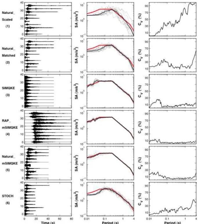
Table 2.2 presents the means and variabilities of the three intensity measures considered when simulating the nonstationary stochastic accelerograms for the six sets of time-histories. Figure 1 presents the accelerograms and spectra of the six sets and as a measure of the variability in the spectra within each set, the coefficients of variation for spectral acceleration. From Table 2.2 and Figure 1 it can be seen that the Natural_Scaled set shows the greatest variability and the SIMQKE records the least, with the other sets somewhere in between. It will be shown subsequently that this variability in input records carries over to variability in building and site response.
Table 2.2: Means and variabilities of three key strong-motion parameters for the six sets of records Ln(PGA) Ln(AI) Ln(SMD) Exp(µ) (m/s2) Exp(") Exp(µ) (m/s) Exp(") Exp(µ) (s) Exp(") 1 Natural_Scaled 2.15 1.00 0.33 1.80 7.24 1.74 2 Natural_Matched 2.23 1.16 0.29 1.51 7.66 1.63 3 SIMQKE 2.20 1.00 0.69 1.20 7.65 1.02 4 RAP_mSIMQKE 2.36 1.06 0.90 1.22 16.41 1.29 5 Natural_mSIMQKE 2.53 1.14 0.51 1.28 8.74 1.38 6 STOCH 2.19 1.04 0.36 1.15 7.59 1.17
Figure 1. Left: The 6 sets of accelerograms generated for the nonlinear dynamic analyses. Middle: Corresponding response spectra (gray), geometric mean of response spectra (black) and EC8 design
spectrum for type B soil (red). Right: Coefficient of variation of spectral acceleration.
3. ANALYSIS OF BUILDING RESPONSE
In this section some analyses of building response using the six sets of acclerograms are presented. We have chosen to conduct relatively simple structural modeling because of the number of runs that are required but we believe that the general trends observed will carry over to more sophisticated dynamic analyses.
3.1. Method
It is well known that structures do not remain elastic under strong shaking. To compare the effect of the six sets of accelerograms presented above, we compute the non-linear response of SDOF systems. The building behaviour is described following a model developed to simulate hysteretic energy capacity. In this paper, we used the Takeda model, first proposed by Takeda et al. (1970) and since analysed in depth by Schwab and Lestuzzi (2007) and Lestuzzi et al. (2007). The Takeda model includes realistic conditions for the reloading curves that model the characteristics of reinforced concrete better than the standard elasto-plastic model. The Takeda model also accounts for the degradation of the stiffness with increasing excitation, which is related to the opening and closing process of existing cracks in the concrete, i.e. a reduction in the natural frequency of the building is accounted for. This behaviour is often observed in real structures under intense loading.
Five parameters are used to describe the Takeda-model: the initial stiffness related to the natural frequency of the SDOF, the yield displacement (Ulin=0.002m), the post-yield stiffness corresponding here to 5%, the coefficient # related to the stiffness degradation and the target $ of the reloading curve. In this study, standard values are used to develop the Takeda model: # = 0.4 and $ = 0.0. The strength reduction factor R is 2, i.e. considering a structure having limited hysteretic energy dissipation capacity, and currently recommended by design codes.
For each set of accelerograms, three initial frequencies are considered, 1Hz (1s), 2Hz (0.5s) and 5Hz (0.2s) roughly corresponding to frequencies of low- and medium-rise reinforced-concrete (RC) buildings. A damping coefficient of 5% is used, which is standard for RC structures.
3.2. Results
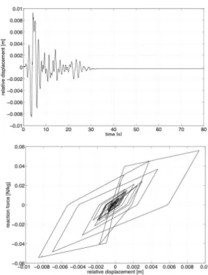
Figure 2 shows the force-displacement of the Takeda-model for the Parkfield record (#1, Table 2.1) and the 1Hz SDOF. We observe the hysteretic loops of the non-linear behaviour of the system. The relative displacement of the SDOF is also shown in Figure 2 (upper row), this parameter being chosen to compare the effect of the variability of the seismic ground motion in building response.
Figure 2. Example of relative displacement (upper figure) and force-displacement curve (lower figure) for the 1Hz SDOF building using the Parkfield record (#1 Table 1).
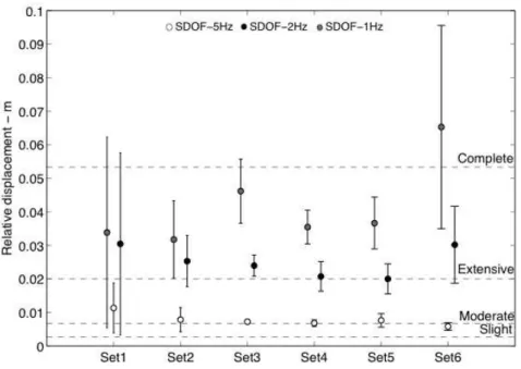
Considering the six sets of accelerograms analysed in this paper, the three SDOF are tested and the relative displacements are compared (Figure 3). We observe higher variability in the building response for natural accelerograms (sets 1 and 2). This indicates that natural variability should be accounted for when selecting accelerograms and using synthetic time histories partially reduces the variability of the structural response (i.e. sets 3, 4 and 5). In addition, the variability of the relative displacement increases for long-period buildings (1Hz). Depending on the features of the buildings, if this variability is neglected, the computed building response may underestimate the building response and the post-earthquake integrity of the building. Also depending on the set of accelerograms, the relative displacement may be much larger than the drift ratios used to define median values of structural damage, considering the category of shear-walls RC buildings, with moderate elevations defined by HAZUS (C2M type). We observe that the damage state of the building can be greatly underestimated when the ground-motion variability is not considered.
Figure 3. Comparison of the relative displacement computed for 1Hz (gray), 2Hz (black) and 5Hz (open) buildings, for the six sets of accelerograms. The dotted lines correspond to the inter-story drift ratios suggested by HAZUS and used to define median values of structural damage (Slight, Moderate, Extensive and Complete)
for C2M buildings.
4. ANALYSIS OF SOIL RESPONSE
Because nonlinear dynamic analyses are not only commonly conducted for building response but also for geotechnical studies, in this section the response of soil layers are analyzed using the same six sets of accelerograms.
4.1. Method
The multi-shear mechanism model (Towhata and Ishihara, 1985) is a plane-strain formulation to simulate pore pressure generation in sands under cyclic loading and undrained conditions. Iai et al. (1990a, b) modified the model to account for the cyclic mobility and dilatancy of sands. The multiple mechanism model relates the stress " and strain % through the following incremental equation (Iai et al., 1990a, b):
where the curly brackets represent the vector notation; {%p} is the volumetric strain produced by the pore pressure, and [D] is the tangential stiffness matrix. This matrix is composed by the volumetric and shear mechanisms, which are represented by the bulk and tangential shear moduli, respectively. The latter is idealized as a collection of I springs separated by &' = ( / I (Figure 4). Each spring follows the hyperbolic stress-strain model (Konder and Zelasko, 1963) and the generalized Masing rules for the hysteresis process (O’Connell et al., 2012). For more details on the model the reader is referred to Iai et al. (1990a, b).
Figure 4. Schematic figure for the multiple simple-shear mechanism. The plane strain is the combination of pure shear (vertical axis) and shear by compression (horizontal axis) (after Towhata and Ishihara, 1985).
Iai et al. (1995) thoroughly studied the soil response at Kushiro Port during the Kushiro-Oki M7.8 1993 earthquake. The soil column is composed of dense sands where the first 30 m are suspected of having strong dilatancy effects. In this paper, we use the same velocity model assumed to be overlaying EC8 site class B material with a shear wave velocity of 500 m/s so that it is consistent with the accelerograms chosen above. Furthermore, we keep Iai et al. (1995) dilatancy parameters to simulate pore pressure changes in the soil column in the first 30 m depth. As an input motion we use the 60 acceleration time histories presented in Section 2. The boundary condition at the bottom of the soil column is assumed to be an elastic boundary condition (outcrop ground motion). The incident wavefield is divided by two before computing wave propagation in order to remove the free-surface effect.
4.2. Results
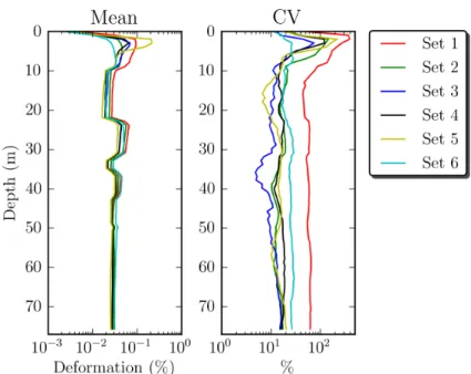
The results of all computations are presented in terms of maximum shear deformation as a function of depth and response spectra of the resulting ground motion at the surface. Figure 5 (left) shows the geometric mean distribution of shear strain versus depth for each input set. Figure 5 (right) shows the coefficient of variation (CV) for each dataset. These results indicate that soil response is sensitive to the chosen acceleration time history in spite of having the same response spectrum. The large values of CV for natural time-histories indicate that natural variability should be taken into account when selecting spectrum-compatible accelerograms. In addition, this dispersion increases in layers where pore pressure effects take place. If this variability is neglected, the computed soil response may underestimate quite considerably the soil deformation.
Figure 5. Distribution of maximum shear deformation versus depth (left). Each line corresponds to the geometric mean strain of each dataset (Table 2.2). Coefficient of variation versus depth for each computed
dataset (right).
Figure 6 shows the geometric mean response spectra (left) and the corresponding CV (right) for the time histories obtained at the surface for each dataset. These results are informative and show the complexity of ground-motion prediction when nonlinear soil behaviour takes place. Indeed, there is a partial correlation between the values of CV and the resulting ground motion at the surface. For example, the natural data (Set 1, red curve), which show the largest variability (CV) do not lead to the highest response spectrum. This can be explained by looking at Figure 5 where the shear strain is largely mobilized by this dataset, thus strong nonlinearity occurs thereby reducing the computed ground motion at the surface. Conversely, the dataset having the smallest CV (Set 5, yellow curve) has almost the largest response at the surface together with dataset 3 in blue. A special case is the one obtained using the nonstationary stochastic accelerograms because these records produce the lowest strains and surface ground motion; yet, its CV in terms of response spectra lies in the middle of other cases (Set 6, cyan curve).
Figure 6. Mean response spectra of computed ground motion at the surface (left) and the corresponding coefficient of variation (right).
resulting response spectra are relatively close. Nevertheless, these results suggest that care should be taken in selecting compatible time histories for soil response that includes nonlinear effects. Few computations may not be enough, thus it is probably a good idea to use several input ground motions in order to see and quantify the dispersion of the resulting ground motion at the surface.
5. CONCLUSION
This study shows that the selection of accelerograms is a fundamental component in earthquake engineering analyses. Using various techniques we have generated six sets of accelerograms following the Eurocode 8 (EC8) guidance (i.e. with the constraint that their response spectra match the EC8 design spectrum) for a B site class, and analyzed their impact on non-linear structures and soil columns. In both cases the variability of the non-linear response highly depends on the set of input accelerograms. It is thus crucial to select sets of accelerograms that represent the natural ground-motion variability.
Since the number of real accelerograms is sometimes limited for a given scenario, an alternative approach is to use nonstationary stochastic simulations (Laurendeau et al., 2011). This technique allows the rapid generation of many sets of “realistic” accelerograms with chosen variability of ground-motion parameters. For instance, the results presented in this paper could be expended to sites of classes A, C and D deploying stochastic simulations with ground-motion indicators calibrated using the PEER database, in which a large number of records are available for class B sites.
AKCNOWLEDGEMENT
This work was sponsored by the Ministry of Sustainable Development through the French Accelerometric Network working group (Seismic ground motion for engineering)
REFERENCES
Abrahamson, N. A. and W. J. Silva (1996). Empirical ground motion models, Report to Brookhaven National
Laboratory.
Douglas, J. (2006). Strong-motion records selection for structural testing. Proceedings of First European
Conference on Earthquake Engineering and Seismology (a joint event of the 13th ECEE & 30th General Assembly of the ESC). Paper number 5.
Douglas, J. and H. Aochi (2008). A survey of techniques for predicting earthquake ground motions for engineering purposes, Surveys in Geophysics, 29:3, 187-220. DOI 10.1007/s10712-008-9046-y.
Federal Emergency Management Agency (FEMA) (1999). HAZUS Earthquake loss estimation methodology. Federal Emergency Management Agency, Washington, D.C.
Gasparini, D. A. and E. H. Vanmarcke (1976). SIMQKE: A Program for Artificial Motion Generation, Department of Civil Engineering, Massachusetts Institute of Technology, Cambridge, MA.
Iai, S., Y. Matsunaga, and T. Kameoka (1990a). Strain space plasticity model for cyclic mobility, Report of the
Port and harbour Research Institute, 29, 27-56.
Iai, S., Y. Matsunaga, and T. Kameoka (1990b). Parameter identification for cyclic mobility model, Report of the
Port and harbour Research Institute, 29, 57-83.
Iai, S., T. Morita, T. Kameoka, Y. Matsunaga, and K. Abiko (1995). Response of a dense sand deposit during 1993 Kushiro-Oki Earthquake, Soils and Foundations, 35, 115-131.
Konder, R.L. and J.S. Zelasko (1963). A hyperbolic stress-strain formulation for sands, in Proc. Of 2nd Pan American Conference on Soil Mechanics and Foundation Engineering, Brazil, 289-324.
Laurendeau, A., F. Bonilla, and F. Cotton (2011). Seismic Indicators Prediction Equations for Japan, Abstracts of the SSA Annual Meeting, Seismological Research Letters, 82:2, 319.
O’Connell, D., J.P. Ake, L.F. Bonilla, P. Liu, R. LaForge, and D. Ostenaa (2012). Strong ground motion estimation, in Earthquake Research and Analysis – New Frontiers in Seismology, ISBN 978-953-307-840-3.
Pequegnat C., Gueguen P., Hatzfeld D., Langlais M. 2008. The French Accelerometric Network (RAP) and National Data Centre (RAP-NDC). Seismological Research Letters, 79:1, 79-89.
Pousse, G., Bonilla, L. F., Cotton, F., Margerin, L. (2006). Nonstationary stochastic simulation of strong ground motion time histories including natural variability: Application to the K-net Japanese database. Bulletin of
the Seismological Society of America, 96, 2103–2117.
Towhata, I. and K. Ishihara (1985). Modeling soil behavior under principal axes rotation, paper presented at the
Fifth International Conference on Numerical Methods in Geomechanics, Nagoya, Japan, 523-530.
Lestuzzi, P., Y. Belmouden and M. Trueb (2007). Non-linear seismic behavior of structures with limited hysteretic energey dissipation capacity, Bull. Earthquake Eng., 5:1, 549-569.
Takeda, T. M.A. Sozen and N.M. Nielsen (1970). Reinforced concreete response to simulated earthquakes. J.
Struct. Div. 96(ST12). Proceedings of the American Societey of Civil Engineers (ASCE).
Schwab, P. and P. Lestuzzi (2007). Assessemnt of the seismic non-linear behavir of ductile wall structures due to synthetics earthquakes, Bull. Earthquake Eng., 5:1, 67-84.