Detection of launch frame in long jump videos using computer vision and discreet computation

Detection of Launch Frame in Long Jump Videos Using Computer Vision and Discreet Computation

MASSACHUSETTS INSTITUTE OF TECHNOLOGY by

JUL 16 2019

LIBRARIES

Department of Mechanical Engineering

In Partial Fulfillment of the Requirements for the Degree of Bachelor of Science in Mechanical Engineering

at the

Massachusetts Institute of Technology June 2019

C 2019 Massachusetts Institute of Technology. All rights reserved.

Signature redacted

Signature of Author:

Department of MechanicA ngineering May 10, 2019

Signature redacted

Certified by:

Anette Hosoi Associate Dean of Engineering/Professor Thesis Supervisor

Signature redacted

Accepted by:

Maria Yang Associate Professor of Mechanical Engineering

Detection of Launch Frame in Long Jump Videos Using Computer Vision and Discreet Computation

by Pablo E. Muniz

Submitted to the Department of Mechanical Engineering On May 10, 2019 in Partial Fulfillment of the

Requirements for the Degree of

Bachelor of Science in Mechanical Engineering

ABSTRACT

Pose estimation, a computer vision technique, can be used to develop a quantitative feedback training tool for long jumping. Key performance indicators (KPIs) such as launch velocity would allow a long jumping athlete to optimize their technique while training. However, these KPIs need a prior knowledge of when the athlete jumped, referred to as the launch frame in the context of videos and computer vision. Thus, an algorithm for estimating the launch frame was made using the OpenPose Demo and Matlab. The algorithm estimates the launch frame to within 0.8t0.91 frames. Implementing the algorithm into a training tool would give an athlete real-time, quantitative feedback from a video. This process of developing an algorithm to flag an event can be used in other sports as well, especially with the rise of KPIs in the sports industry (e.g. launch angle and velocity in baseball).

Thesis Supervisor: Anette Hosoi

Acknowledgements

The author would like to thank Prof. Anette (Peko) Hosoi for her indispensable guidance throughout the term of this project. He would also like to thank Phil Cheetham for advice

regarding long jumping and for allowing the author to use the USOC's training videos. Additional thanks to Golda Nguyen and Jeremy Storming for their work with OpenPose and gathering the data for this application.

Table of Contents Abstract 3 Acknowledgements 4 Table of Contents 5 List of Figures 7 List of Tables 8 1 Introduction 9

2 External Feedback, OpenPose, and Long Jumping 9

2.1 External Feedback While Training 9

2.2 OpenPose and Computer Vision 10

2.3 Long Jumping Rules and Technique 11

2.4 Regressions 12

2.4.1 Linear Regressions 12

2.4.2 Quadratic Regressions 13

3 Experimental Design 14

3.1 Manually Detect Launch Frame and Launch Foot 15

3.2 Removing Outliers 15

4 Algorithm Development and Testing 17

4.1 Breakpoints K 17

4.2 Aggregate Phase Regression (2 Breakoints per signal) 17 4.3 Aggregate Phase Regression (3 Breakpoints per Signal) 19

5 Conclusions 25

6 Appendices 26

Appendix A: Code 26

Appendix B: Sample OpenPose Data 43

List of Figures Figure 1-1: Figure 2-1: Figure 2-2: Figure 2-3: Figure 2-4: Figure 2-5: Figure 3-1: Figure 4-1: Figure 4-2: Figure 4-3: Figure 4-4: Figure 4-5: Figure 4-6: Figure 4-7: Figure 4-8: Figure 4-9:

Long jump world record progression OpenPose output signals

OpenPose applied to long jumping Long jump distance model

Linear regression example Quadratic regression example

OpenPose data with and without outliers Breakpoint definition

Video 7 Aggregate RSS 2 Bkpts results Aggregate RSS 2 Bkpts LFE magnitude Modified breakpoint definition

Video 8 Aggregate RSS 3 Bkpts results Aggregate RSS 3 Bkpts LFE magnitude

Aggregate RSS 3 Bkpts left foot LFE magnitude

Video 3 Multiple Signal Aggregate RSS 2 Bkpts results Multiple Signal Aggregate RSS 2 Bkpts LFE magnitude

9 10 11 11 13 14 16 17 18 19 20 21 22 22 24 24

List of Tables

I

Long jumping is a track-and-field sport that consists of a horizontal jump following a running start with the goal of jumping the farthest. An Olympic sport since antiquity, it was part of the 708 BC Olympic games and it is still practiced to this day [1]. Long jumping has become more competitive in recent decades since professional Olympic committees have become the norm, leading to more accurate selection of the best athletes. As shown in Figure 1-1, technological advancements have increased the efficacy of training regiments, pushing athletes' bodies to their limit and lengthening world records. Nevertheless, there is still a dearth of quantitative, external feedback

9

Long Jump World Record Progression 8.51 E7 - 6 8 .5 7 .51-6

|-Men

-Women World Record

1920 1940 1960 1980 2000 2020 Year

Figure 1-1: Long jumping world record progression since 1900. As in

most sports, long jumping athletes have become more proficient with more efficient training, increasing the sport's competitiveness. Data. [2]

training tools [3]. This can be filled with the advent of computer vision programs.

Computer Vision is a branch of computer science that attempts to give computers the ability to see videos and pictures. OpenPose, a computer vision program developed in Carnegie Mellon University, does pose estimation, allowing a computer to estimate the position of 25 key body parts. This program was used to acquire the data for this application. The KPIs representative of success in long jumping are velocity and angle when jumping: launch velocity and launch angle, which are calculated from the frame in the video where the athlete starts jumping, referred to as the launchframe. We develop an algorithm that provides an accurate estimate of the launch frame using six of these discreet time signals (left/right ankle, heel, and toe) in order to make these KPI calculations automatically and accurately.

2. Feedback, OpenPose, and Long Jumping 2.1 Feedback While Training

Traditionally, feedback in sports has taken the form of a coach's verbal feedback based on qualitative results or their own perception of an athlete's performance. This process is

inherently qualitative and is dependent on a coach's ability to notice and communicate what they see. However, the development of sensory instrumentation has allowed athletes and their coaches to study their bodies' kinematics in newly quantitative terms. Along with an increased

understanding of biomechanics, athletes have been able to use this data to improve their techniques.

In addition, athletes have benefitted from having access to this data in real-time (e.g. heart-rate monitor, accelerometers, etc.). A study by Anderson, Harrison, and Lyons (2005) tested the benefits of real-time feedback and summary feedback on 13 experienced rowers. They concluded that real-time feedback significantly increased the consistency of the rowers'

technique over no feedback. In addition, summary feedback also provided more consistent results than training with no feedback [4]. A similar study by Eriksson, M., Halvorsen, K. A., and Gullstrand, L. (2011) tested how real-time feedback affected 18 trained runners' ability to maintain a consistently optimal running form. In almost all cases, the athlete was successful in

5.5 51i

correcting their running form [5]. Although quantitative external feedback can be invaluable to an athlete, it has to be accurate and relevant, appropriately timed, and decipherable to the athlete

[6]. Therefore, key performance indicators (KPIs) that are indicative of good performance should be used to simplify the feedback data, ensuring these three conditions are met.

2.2 OpenPose and Computer Vision

Although sensory instrumentation has become smaller and lighter over time, it can still inhibit an athlete's movements and affect their performance. In order to optimize a technique for competition, it is important to recreate a competition's condition (i.e. no sensors). Therefore, there is a need for non-invasive quantitative feedback systems such as computer vision programs coupled with discreet-data algorithms. By giving the computer the ability to see how a person is moving, we can give it the ability to compute long jumping's KPIs by simply processing a video.

OpenPose was used to estimate the location of a long jumper's key body parts in a video frame. As seen in Figure 2-1, the OpenPose demo outputs the approximate location of 25 key body parts in each of the video's frames. The 10 videos used as data to develop this application were from this perspective: to the side of the athlete.

Figure 2-1: (left) The 25 signals tracked by the OpenPose demo are shown [7. We will use the foot

coordinates for this application, but the rest can be used to estimate the center of mass's location. (right) Example of how the OpenPose demo works on one of our ten long jumping videos

For general pose detection, OpenPose creates a 3-point vector of <x, y, confidence level> for each body part detected (total of 25 body parts detected), and the parts are ordered and named in the output file as follows [7]:

0) Nose

3) Right Elbow (RElbow) 6) Left Elbow (LElbow) 9) Right Hip (RHip)

12) Left Hip(LHip)

15) Right Eye (REye) 18) Left Ear (LEar) 21) Left Heel (LHeel)

24) Right Heel (RHeel)

1) Neck

4) Right Wrist (RWrist)

7) Left Wrist (LWrist) 10) Right Knee (RKnee) 13) Left Knee (LKnee) 16) Left Eye (LEye)

19) Left Big Toe (LBigToe)

22) Right Big Toe (RBigToe)

2) Right Shoulder (RShoulder)

5) Left Shoulder (LShoulder)

8) Mid Hip

11) Right Ankle (RAnkle)

14) Left Ankle (LAnkle)

17) Right Ear (REar)

20) Left Small Toe (LSmalIToe)

2.3 Long Jumping Rules and Technique

The standard setup for a long jumping competition is a runway with a sand landing pit adjacent to it. As seen in Figure 2-2, there is a foul line at the end of the runway and the athlete's foot must be behind it for the attempt to be valid. The measurement begins where the foul line ends, so jumping as close to it as possible is ideal. In addition, long jumpers usually receive three opportunities to complete a valid attempt in each round. Therefore, it is essential for a long jumper to consistently perform their technique.

Figure 2-2: (left) Picture of long jumping setup.[8] (right) Model of long jumping setup, the measurement board displays the jumping distance the athlete is attempting to maximize. [9]

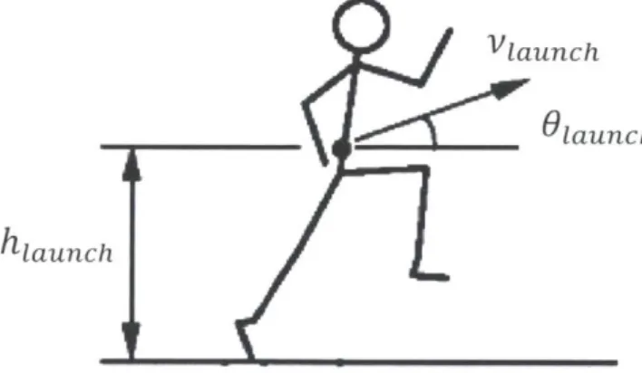
Modeling long jumping distance dfinal requires knowledge of some key variables: center

of mass (COM) position at launch (0 , hlaunch), COM speed at launch Vlaunch, and angle of launch 0

launch. Accordingly, knowing when the take-off occurred is paramount. Since this

application uses videos, this is referred to as the launchframe. Figure 2-3 is a graphical representation of our long jumping model with the defined parameters.

Vlaunch

L Olaunch

hiaunch

Figure 2-3: Model of long jumping at the launch frame, where our desired KPIs are displayed. [10]

The center of mass's height at launch hlaunch is inherent to the athlete so it cannot be

easily changed by changing techniques. However, Vlaunch and 6

launch can be altered with a change in technique, making them the relevant KPIs for long jumping performance. The long jumping distance dfinal is then given by (Linthorne et al, 2005) [10]:

1

"a sinziaunc1) 2h

12

sin26an + sin 2 ₀

(1)

Where g is the acceleration due to gravity (9.81m/S2) and relative h is given by:

h = hlaunch - hlanding (2)

According to Linthorne, Guzman, and Bridgett, the optimal launch angle is not the expected 450. The launch velocity for a jumper decreases as the launch angle increases, so for most jumpers the optimal launch angle is approximately 220 [10].

2.4 Regressions

Regressions are the optimization of a model curve f(T) such that it approximates the original data (T, Y) as best as possible. Since we are working with videos, T will be an array of the video's frames, where n is the total amount of frames in each video. This is shown in equation 3:

T= [12 ... n] (3)

Usually, regressions are optimized by minimizing the error between the model curve and the original signal. Since the error can be both positive and negative, it is commonplace to use the Residual sum of squares (RSS) to model the error. This can be seen in equation 4:

n

RSS=

Z

Y

i=1

The model curve used can be composed of a linear combination of functions of T. To get the best results, it is ideal to choose the functions to use in any regression based on the data it is trying to approximate. In this application, we used linear and quadratic regressions.

2.4.1 Linear Regression

In a linear regression, the model curve will have the form of a linear equation, shown in equation 5:

Y(T)

n

RSS = [Yi -

(O

Ti

P2)]

i=1

This can be solved with matrix division. We define To as:

[T

1

T = 2 1. (7) TTO1

To solve for the pair of coefficients ( 1, 2) that minimize the RSS, we need to solve the relationship in equation 7:

Y = Tfl where

fl =

E

2

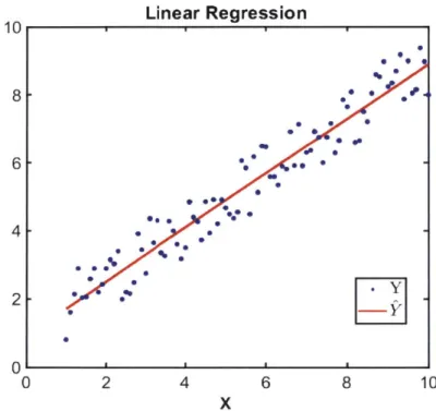
The Matlab function "regress(Y, X)" returns an array ft that minimizes any residual error RSSI. An example of an implementation of the regress Matlab function can be seen in Figure 2-4. 10 8 6 4 0 Linear Regression . *0 .* *. . 0 . .. g .*.*0. -S 0 2 4

X

Figure 2-4: Result of linear regression on a discrete line where random noise was added results in an

approximation of the original line.

2.4.2 Quadratic Regression

When making a quadratic regression, the model signal Y will take the form:

Y(T)

flT

2T+ f3

Similar to the linear regression, the RSS is given by: n

RSSq = Y- (f 1T.2

(9)

(10)

+ 2Ti i +

/3)]

The Matlab function "fit(X, Y,'poly2')" will return a vector ft that minimizes the error RSSq where:

f

=

/2]

W3

A second order polynomial is commonly used to model a projectile's center of mass

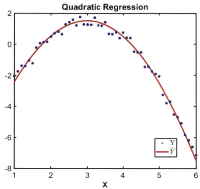
y-coordinates. A second order regression is warranted when data collection leads to some error in data. An implementation of this using the Matlab function can be seen in Figure 2-5.

2 0 -2 -4 -6 -8 1 Quadratic Regression see _e 2 3 4 5 6 X

Figure 2-5: Result of quadratic regression on a discrete second order polynomial where random noise

was added results in an approximation of the original polynomial.

3 Experimental Design

The goal was to develop an algorithm that will receive the athlete's coordinates as an input and output an estimate the launch frame. First, we needed accurate 'baseline' data to develop and corroborate the algorithm's efficacy. As discussed in Section 2.2, the OpenPose Demo was used as the data collection method and all the analysis was done in Matlab. Matlab was also used to produce the figures and the algorithm estimating the launch frame. The OpenPose data was processed to remove outliers. Only the foot signals for each foot (L/R Toe, L/R Ankle, L/R Heel) were used for the purpose of estimating the launch frame.

3.1 Manually Detect Launch Frame and Launch Foot

The true launch frame and launch foot were found by looking at the videos frame-by-frame using the Tracker Video Analysis and Modeling Tool [11]. The data points at the launch frame were highlighted by a red data point on all graphs to help identify trends that could be exploited in the algorithm. The actual launch frame and foot of the 10 videos analyzed are shown in Table 3-1.

Video # Actual Launch Frame Actual Launch Foot

1 28 Left 2 33 Left 3 26 Left 4 22 Left 5 34 Left 6 19 Left 7 22 Left 8 23 Left 9 30 Left 10 13 Left

Table 3-1: Actual launch frame and launch foot from each video, generated from looking at each video frame by frame.

3.2 Removing outliers

Since OpenPose's machine learning algorithm was not trained using long jump videos, it sometimes outputs data points that are incorrect for this application. Some coordinates are read at 0, resulting in a non-continuous curve. This happens in both x and y coordinates and could lead to inaccuracies when detecting the launch frame. Since the data is taken from a long jumping video, we expect the data to be continuous. Thus, the spikes in the raw OpenPose data are erroneous data points that were replaced by interpolation. A comparison of the OpenPose data before and after the outliers were removed and interpolated over is shown in Figure 3-1.

Videol Left Toe 1500 M 1000 C 500 0 0 -200 S -400 -600 1500 M 1000 C 8500 x 0 0 ca-200 -400 -600 1500 1l) cc 1000 C 500 0 0 c -200 -400 -600 0 20 40 60 Index .S , Cu 8 -6 X 1500 -1000 -500 -0 120 20 40 60 80 100 Index 20 40 60 80 100 Index

Videol Left Ankle

0 20 40 60 80 100

Index

0 20 40 60 80 100

Index

Videol Left Heel

0 20 40 60 80 100 Index

-u

Videol Left Ankle 1500 1000 500 -0 0 20 40 60 80 100 12 Index -400 -450 120 0 20 40 60 Index

Videol Left Heel

- 1500 U a, 120 10 500 -0 20 40 60 Index "2) 80 100 120 450 -500 0 80 100 120 80 100 0 20 40 60 80 100 Index

Figure 3-1: (left) Each of video l's left foot raw signals as returned from the OpenPose demo. (right) The same signals with outliers removed. The red dot corresponds to the actual launch frame shown in Table 3-1.

-400

-450

. ...

Video1 Left Too

These plots led us to believe the y-coordinates were more representative of the launch. That is, the data had distinctions around the launch frame that could be tested in an algorithm. In this

case, all of the y-coordinate plots had a parabolic-shaped bump immediately after the launch frame, shown by the red dot. Therefore, we exclusively worked with y-coordinate data for the rest of the process.

4 Algorithm Development and Testing

We designed three algorithms and wrote Matlab code that implements each one. We then ran the OpenPose data from our ten long jump videos through this code to test each one's

efficacy.

4.1 Breakpoints K

The y-coordinates graphs have 3 phases: pre-jump, jump, post-jump. Breakpoints are the frames where one phase ends and another begins. Most videos show the beginning of the second phase coinciding with the actual launch frame. An example of one such signal is shown in Figure 4-1. Breakpoint Definition -400 2 -450

-8

Figure 4-1: The actual launch frame is depicted by the red dot. In addition, the three defined phases are

shown by the three colored, horizontal lines. Yellow is the first phase (1 to kl), red is the second phase (k1 + 1 to k2), and purple is the third phase (k2 + 1 to end). The breakpoints k, and k2 are shown on the

horizontal axis.

4.2 Aggregate Phase Regression (2 Breakpoints per signal)

First, we chose to model the y-coordinates' phases by a line, a parabola, and a line, respectively. The goal was to choose optimizing breakpoints for each signal that would minimize the error between our estimated curve and each of the foot signals. Thus, we tested different

combinations of possible breakpoints k = (kl, k₂) and performed two linear and one quadratic regressions at each combination k. In each trio of regressions, we stored the Aggregate Residual Sum of Squares (RSSA), given by equation 12; where RSS11 is the RSS of the first linear

regression, RSSq is the RSS of the quadratic regression, and RSS12 is the RSS of the second

RSSA = RSS11 + RSSq + RSS₁₂

This definition of the Aggregate Residual Sum of Squares can be expanded into equation 13 to better understand the algorithm.

RSSA

Z(Y

_-

_ii()

i=1 n ) 2

+

(Y

In this definition, n is the number of toe, heel, or ankle coordinates, T = [1 2 ... n] is the vector of frames, Y = [Y Y2 ... Yn] is the vector of y-coordinates at each frame, and Y1, Yq, Y2

are the model curves given by each regression. After testing each possible combination of k, we chose the one with the smallest RSSA as our optimized breakpoints kopt. The launch frame is the first of these optimized breakpoints k1jpt. Figure 4-2 shows the results of this algorithm on each foot signal in video 7.

Video 7 -350 -400 -450 -500 -550

Launch Frame Est. 26

0 10 20 30 40 50 60

Frames

Launrch Fram. Esnt24

-350 -400 450 -500 -550 -350 -400 I j-450 -500 -550 " " " " " 0 10 20 30 40 50 60 Frames

Launch Frame Est. 24

-350 r , - .-. -400 -450 -500I .550 --- - -0

Launch Frame Est. 23

0 10 20 30 40 50 60

Frames

Launch Frame Est. 27

C M -450 -500 -550 0 10 20 30 40 50 60 Frarmes

Launch Frame Est. 27 -350 -400 0-450 -500 -550-10 20 30 40 50 60 0 10 20 30 40 Frames Frames

Figure 4-2: The results of running the data from video 7 through the algorithm. k, for each signal is shown at

the top of each subplot. As can be seen, the quadratic region was not estimated how we expected. The estimated curve in each phase is depicted by the same colors as in Figure 4-1.

(12)

(13)

0

-1

The optimizing break points were not as hypothesized in Figure 4-1. Ideally, the quadratic regression region, shown in red above, would be concave and symmetric around the vertex. However, as seen in the Right Heel plot (bottom right), this is not always the case. This is

likely due to noise from pose estimation and modeling the foot coordinates instead of the center of mass coordinates. This algorithm was run on the 6 signals in each of the 10 videos and we compiled the Launch Frame Error (LFE) for each signal, given by equation 14.

LFE = k1 - (Actual launch

frame)

The Launch Frame Error magnitude for each signal is shown in Figure 4-3.

Unear-Quad-Lin Error Magnitude

Video 1 Video 2 30 ]Video 3 Video 4 Video 5 =~]Video 6 Video 7 Video 8 25 - Video 9 [=]Video 10 -- Average ~20 a0 1 C 10-10 5

Lank Lheel Ltoe Rank Rheel Rtoe

Signals

Figure 4-3: Launch Frame Error magnitude for each signal (horizontal axis) and each video (legend). Note that the left foot estimates are much better. It is also important to note that this is the absolute value error, as the error can be either positive or negative. The average error foe each signal is shown by the red line.

The estimated launch frame performed well (I LFE 1=3) as long as we look at signals given by the correct launch foot, which is the left foot in video 7. In addition, the average error magnitude was the same for each of the left foot signals, leading us to believe that none of the signals was more representative than the other two. There is also the need to decide how to estimate the video's launch frame from each signal's k1.

4.3 Aggregate Phase Regression (3 Breakpoints per Signal)

We simplified the definition of phases and breakpoints to mitigate the pose estimation's noise. Instead of modeling the signal with 2 linear regressions and 1 quadratic regression, we chose to do so with 4 linear regressions. Therefore, we now expected 4 phases, defined in Figure 4-4.

Modified Breakpoint Definition

0 20 ki k2 k3 80 100

Index

Figure 4-4: The actual launch frame is depicted by the red dot. In addition, the four defined phases are shown by the four colored, horizontal lines. Yellow is the first phase (1 to kj), red is the second phase (k₁ + 1 to k₂), purple is the third phase (k2 + 1 to k3), and green is the fourth phase (k3 + 1 to end). The breakpoints kj, k2and k2are shown on the horizontal axis.

Similarly, our Aggregate Residual Sum of Squares definition was changed new breakpoint definition. This is shown in equation 15, where RSS1 is the linear each phase.

to reflect the regression in

RSS = RSS ₁ + RSS12 + RSS13 + RSS14

Our expanded Aggregate Residual Sum of Squares definition is given by equation 16.

RSSA _(Yi i=1

+i

~

+

2(T

In this definition, n is the number of frames, T = [1 2 ... n] is the vector of frames,

Y = [Y1 Y2 ... Yn] is the vector of y-coordinates at each frame, and -1, Y12, 13, 14 are the model

curves given by each regression. After testing each possible combination k = (kj, k2, k3), we

chose the one with the smallest RSSA as our optimized breakpoints kopt. The launch frame is the first of these optimized breakpoints k1,,pt. Figure 4-5 shows the results of this algorithm on each foot signal in video 9.

-400 -450 W, a). I I I I I I I I I -500 120 (15) n i=k3+1

Video 9 Launch Frame Est. 7

-400 1 Fraes 4 . -45

-I

-400

Q -450 -500 ____________

0 10 20 30 40 50 60

Frames

-30Launch Frame Est. 31______ -400 -450

-50

Launch Frame Est. 30

-350 -400 -450 -500 -550 0 10 20 30 40 50 60 Frames Launch Frame Est. 14

-550-0 10 20 30 40 50 60

Frames Launch Frame Est. 14 350

-550

0 10 20 30 40 50 60

Frames

Figure 4-5: The results of running the data from video 9 through the algorithm. k, for each signal is shown at the top of each subplot. As can be seen, the linear breakpoints align with our theorized phase regions in Figure 4-4. The estimated curve in each phase is depicted by the same colors as in Figure 4-4. Note that the left toe (top left) k, is considerably different than the rest and that the signal does not clearly show the landing.

Using this algorithm, the optimized breakpoints kopt consistently were at the theorized start of each phase. However, video 9, shown in Figure 4-5, had an outlier in the Left Toe

coordinates. We ran the data from each of the 10 videos through this algorithm and compiled the Launch Frame Error, as defined in equation 14. This algorithm's LFE magnitude is shown in Figure 4-6.

Unear Breakpoints Error Magnitude

0

Lank Lheel Ltoe Rank Rheel Rtoe

Signals

Figure 4-6: Launch Frame Error magnitude for each signal (horizontal axis) and each video (legend). Note that the left foot estimates are much better. It is also important to note that this is the absolute value error, as the error can be either positive or negative. The average error foe each signal is shown by the red line.

In video 8, the launch foot is the left foot, which is reflected in Figure 4-6. The algorithm performed better when looking at the left foot's coordinates. The LFE of the left foot's

coordinates are shown in Figure 4-7.

Left Foot Unear Breakpoints En-or Magnitude

-~-

UN

Figure 4-7: Left foot launch frame error magnitude. The outlier in video 9 could severely affect 40 35 30 -=25 -30 1= 20 C 1 -~i 10 5 Video 1 Video 2 L Video 3 Video 4 Video 5 =Video 6 Video 7 Video 8 Video 9 [=]Video 10 -Average 201-Video 1 Video 2 IVideo 3 Video 4 Video 5 [=]Video 6 Video 7 Video 8 Video 9 1 Video 10 -- Average 15 IZ i 5 0 I I I I

The algorithm returned a large outlier in video 9's left toe signal due to noise around the time the athlete landed, damaging the signal. The average LFE for the left toe signals was 2.8 frames while including the outlier and 2 frames not including the outlier. Thus, it performed better than the 2 Breakpoint Aggregate Regression algorithm, but we still have the problem of choosing one launch frame for the video while we have 3 k1s. Bases on these results, we decided

to just use the launch foot coordinates (left foot for our videos) as their results are more accurate. 4.4 Multiple Signal Aggregate Phase Regression (3 Breakpoints per Video)

We decided to design the algorithm such that it will return one combination of optimized breakpoints kort per video. We theorized that it would make the algorithm less sensitive to outliers and that it would be more be more accurate, as we would be using data from 3 signals. We used the same definition for breakpoints as discussed in Figure 4-4, k = (kl, k2, k3), but we

modified our Aggregate Residual Sum of Squares definition to that in equation 17, where RSS1,s is the linear RSS for signal s.

3

RSSA = I RSSs + RSS12,s + RSS 3,s + RSS4,S] (17)

s=1

Again, we can expand this equation to show the algorithm in more detail. This expanded version is given by equation 18. 3 ~k, k2 (18) RSSA -= - (s , + -,s (i,s)2 s=1 Li=1 i=kl+1 k3 n +

I

(

-

(Tis))

+

Y(is)

+ (Yi,s - YsT,s +is -YsT,s

i=k2+1 i=k3+1

In this definition, n is the number of toe, heel, or ankle coordinates, s =

[LToe, Lank, Lheel] is the signals we are using, T = [1 2 ... n] is the vector of frames, Y =

[Y1 Y2 ... Yn] is the vector of y-coordinates at each frame, and Y-, Y-, Y13, Y4 are the model

curves given by each regression. After testing each possible combination k = (kl, k2, k3), we

chose the one with the smallest RSSA as our optimized breakpoints kopt. The launch frame is the first of these optimized breakpoints k1,,pt. Figure 4-8 shows the results of this algorithm on each foot signal in video 9.

-500 -500 -400 -450

F

Estimated Launch Frame:30

I

- 1

_______wIf

-

...

I--

..

I

I

AI

Figure 3-8: The results of running the data from video 9 through the algorithm. k, for each signal is shown at

the top of each subplot. As can be seen, the linear breakpoints align with our theorized phase regions in Figure 4-4. The estimated curve in each phase is depicted by the same colors as in Figure 4-4. Note that the left toe (top left) k, is considerably different than the rest and that the signal does not clearly show the landing.

Adding the Aggregate Residual Sum of Squares between each of the launch foot's signals eliminated the algorithm's sensitivity to noise. In the previous algorithm, the video 9 results, Figure 4-5, had a large outlier in the left toe breakpoints, but this implementation fixed that. The Launch Frame Error magnitude of each video is shown in Figure 4-9.

Cross checked breakpoints Error Magnitude Average Error Mag:0.8

2.5

1-2

1.51

-Video 10 Video 2 Video 3 Video 4 Video 5 Video 6 Video 7 Video 8 Video 9 -400 -450 --I -400 --450 -I I I

1

The average launch frame error magnitude has now been reduced to 0.8 0.91 frames as long as the correct launch foot's signals are used. In this case, all the videos were of an athlete jumping with their left foot. Giving the algorithm access to an athlete's metadata (e.g. what foot

they jump with) would give it the ability to be used while training.

5 Conclusions

An algorithm that consistently provides an accurate estimate for the launch frame from a long jumping video coordinates was made using computer vision and Matlab. With an average launch frame error magnitude of 0.8 0.91 frames, the algorithm can be used to accurately compute launch angle and launch velocity from a long jumping video while avoiding the tedious task of performing the calculations by hand. Consequently, a quantitative, external feedback training tool for long jumping may be within reach.

A

6 Appendices

Appendix A: Code

Find outliers and eliminate with interpolation

Author: Pablo E. Muniz

Date: 03/09/2019

This function takes a struct object of raw OpenPose data and interpolates over outliers. Outliers are data points that

have coordinates at 0. OpenPose has the origin at the top left of a frame by default, so 01 0 is the top of a frame

and (0, a) is the left edge of a frame.

Contents

"

Function definition

function fixedsignal = fix outliers (rawsignal)

Flagging X-coordinates

To find X-coordinate outliers check to see if they are at 0. Add indices where signal is at 0 to index

X = rawsignal.x;

X(isnan(X)) =

index = [];

for i = 1:length(X)

if X(i) == 0

index = [index; ii; end

end

Interpolating X-coordinates

If there are n successive outliers, we want to interpolate over them with non-outliers.

Thus, if Xi, Xi+i, Xi+s- are outliers,

We will use the preceding and following accurate data points: Xi-1 and Xi+n to interpolate.

Find which outliers are successive and which ones are single. Create a vector replace with the staring index and ending index of successive outliers (the start and end index will be the same if it is a single outlier).

We will use recursive programming to make the vector current. The function findsuccessive is shown at the bottom of the document.

replace = [];

Check the indeces in index and run them through findsuccessive

for i = 1:length(index)

[replace,current] = find successive (index(i) ,replace,current);

end

Add the last row from current from the findsuccessive funtion. This needs to be done because of the way

findsuccessive was designed.

if isempty(current) == 0

replace = [replace; current(l) , current(end)]; end

if isempty(replace) == 0

Sample the rows in replace to interpolate over single and successive outliers.

for i = 1:length(replace(:,l))

If the second index in the sampled replace row is the last index, then eliminate these outliers from the signal since we

are not interested in extrapolating.

if replace(i,2) == length(X)

X(replace(i,l):replace(i,2)) = [];

When the first and second index in the sampled replace row are different, this means there are successive outliers. Interpolate using the preceding and following accurate data points: Xi-1 and Xi+n (Trapezoidal method).

elseif replace(i,l) ~ replace(i,2)

X(replace(i,l)-l:replace(i,2)+l) =

linspace(X(replace(i,l)-1),X(replace(i,2)+1),replace(i,2)-replace(i,l)+3);

When the first and second index in the sampled replace row are the same, this is a single outlier. We interpolate using the preceding and following data point (Trapezoidal method).

else X(replace(i,l)) = (X(replace(i,1)-l)+X(replace(i,l)+l))/2; end end end

Y-coordinates

The same process as described above is performed with the Y-coordinates.

Y = raw signal.y;

Y(isnan(Y)) =

for i = 1:length(Y)

if Y(i) == 0

index = [index ; i]; end

end replace =

current = [;

for i = 1:length(index)

[replace,currentl = find successive(index(i),replace,current); end

if isempty(current) == 0

replace = [replace; current(l) , current(end)]; end

if isempty(replace) == 0

for i = 1:length(replace(:,l)) if replace(i,2) == length(Y)

Y(replace(i,l):replace(i,2)) = elseif replace(i,l) ~ replace(i,2)

Y(replace(i,l)-l:replace(i,2)+l) = linspace(Y(replace(i,l)-1),Y(replace(i,2)+l),replace(i,2)-replace(i,l)+3); else Y(replace(i,l)) = (Y(replace(i,l)-l)+Y(replace(i,l)+l))/2; end end end

Construct the fixed struct object to be returned.

fixedsignal.x = X;

fixedsignal.y = Y;

end

findsuccessive

Function definition. num is the index from index being sampled, groups is making replace and current is the last successive data sampled.

function [groups, current] = find successive (num, groups, current)

If current is empty, add the current sampled num index to it.

if isempty(current) == 1

current = [num];

If the index being sampled is right after the last index sampled, update cunent.

elseif current(end) + 1 == num

current = [current ; num];

If the above conditions were not met (if current was not updated), add the last successive indices to replace and

update current.

elseif current(end) num

groups = [groups ; current(l) , current(end)]; current = [num];

end

Find Breakpoints (2 breakpoints:

linear-quadratic-linear)

Author: Pablo E. Muniz Date: 04/14/2019

This function takes a struct object and returns the aggregate Residual Sum of Squares (RSS) between the y-signal

and 3 regressions: linear, quadratic, and linear. It is testing different break point permutations (kI, k2) and returning

the optimal permutation along with the RSS (Rm,). It also creates a plot a with the signal, each of the three

regressions, and the breakpoints.

Contents

"

a Test breakpoint permutations (ki, k₂)

" Regressions

- Picking best breakpoint permutation

* Plotting

Funtion Definition

function [Rmin , k1 , k2 , a] = changepts (signal)

Eliminate outliers and isolate y-signal.

signal no out = fix outliers(signal);

signaly_no_out = signalnoout.y;

Test breakpoint permutations

Lmin is the minimum distance between changepoints and can be modified below depending on choice of speed vs.

accuracy. The vector R will store the RSS and its corresponding permutation of (ki, k2).

R= [];

Lmin 5;

for k1 = 1:numel(signaly no out)-Lmin for k2 = kl+Lmin:numel(signaly no out)

Cut signals into three parts, testing changepoints.

cutl = signalyno_out(1:kl-1);

indecesi = 1:k1-1;

cut2 = signaly_no_out(kl:k2-1); ,am

indeces2 = kl:k2-1;

cut3 = signalynoout(k2:end);

indeces3 = k2:numel(signalynoout);

Regressions

We used Matlab's regress function to perform linear regression: Y =X*3

where X is the indices column vector joined with a column vector of ones and .

We used Matlab's fit function to perform quadratic regression: Regression of first cut

[B1,-,R1] = regress(cutl , [indecesl' , ones(numel(indecesl),i)]); R1 = sum (R1.^2);

Regression of second cut

myfit2 = fit(indeces2' , cut2 , 'poly2'); coeffs = coeffvalues(myfit2);

poly2fit = coeffs(1)*indeces2'.^2 + coeffs(2)*indeces2l + coeffs(3)'; R2 = sum((po1y2fit-cut2).^2);

Regression of third cut

[B3,-,R3] = regress(cut3 , [indeces3' , ones(numel(indeces3),1)]);

R3 = sum(R3.^2) ;

Add error and its corresponding (ki, k2) pairing to existing R.

R = [R ;

Ri+R2+R3 , k1 , k2];

end

end

Picking best breakpoint permutation

The optimizing permutation of (ki, k2) will be the one with the lowest Residual Sum of Squares.

optimized index pair = find(R(:,l) =Rmin);

Ropt = R(optimized index pair,:);

ki = Ropt (2);

k2 = Ropt(3);

Get the fits made with (k1 k) to plot

cuti = signalynoout(l:kl-1);

indecesl = 1:kl-l;

cut2 = signalyno out(kl:k2-1);

indeces2 = kl:k2-1;

cut3 = signaly no out(k2:end);

indeces3 = k2:numel(signalynoout);

[Bl,-,-] = regress(cutl , [indecesi' , ones(numel(indecesl),l)]);

myfit2 = fit(indeces2' , cut2 , 'poly2'); coeffs = coeffvalues(myfit2);

poly2fit = coeffs (1) *indeces2' .^2 + coeffs (2) *indeces2' + coeffs (3) ';

[B3,-,R3] = regress (cut3 , [indeces3' , ones(numel(indeces3),l)]);

Plotting

a = plot (k2*ones(100,1) ,linspace(min(signalynoout)-10,max(signaly_noout)+10,100), 'k-') improvePlot ylim([-510,-390]) xlim( [-1,numel(signalyno_out)+l]) a end

Published with MA TLAB® R201 9a

... ; ... ... ... ;..; ... ... ;.- ... ... ... ... ... s.; ...

Find Break Points (3 breakpoints:

Author: Pablo E. Muniz Date: 04/14/2019

This function takes a struct object and returns the aggregate Residual Sum of Squares (RSS) between the y-signal and 4 linear regressions. It is testing different break point permutations (ki, k2 , k3) and returning the optimal

permutation along with the RSS (Trtl). It also creates a plot a with the signal, each of the four regressions, and the breakpoints.

Contents

* Test breakpoint permutations (ki- k2. k:5

* Regressions

* Picking best breakpoint permutation * Plotting

Function Definition

function [Rmin , kl , k2 , k3 , a] = linearbrkpts (signal) Eliminate outliers and isolate y-signal

signalnoout = fix outliers(signal);

signaly no out = signal no out.y;

Test breakpoint permutations

Lmin is the minimum distance between changepoints and can be modified below depending on choice of speed vs. accuracy. The vector R will store the RSS and its corresponding permutation of (ki, k2, k₃)

Note: Adding limits to what the breakpoints can be makes the function significantly faster, but it runs the chance of the limits being after each breakpoint's mark in the data. These limits were calibrated based on the data available.

R = []; Lmin = 5;

for kl = 1:round(1/2*numel(signaly no out))

for k2 = kl+Lmin:round(6/10*numel(signaly_ noout)) for k3 = k2+Lmin:round(9/10*numel(signaly_noout))

% For no limits on breakpoints:

% for kl = 1:numel(signalyno-out)-2*Lmin

% for k2 = kl+Lmin:numel(signaly no out)-Lmin

% for k3 = k2+Lmin:numel(signalynoout)

Cut signals into four parts:

indecesl = 1:kl-1;

cut2 = signalynoout(kl:k2-1);

indeces2 = kl:k2-1;

cut3 = signaly no out(k2:k3-1);

indeces3 = k2:k3-1;

cut4 = signalynoout(k3:end);

indeces4 = k3:numel(signaly no out);

Regressions

We used Matlab's regress function to perform linear regression:

Y = X *3

where X is the indices column vector joined with a column vector of ones and d I .

Regression of first cut:

[B1,-,R1] = regress(cutl , [indecesl' , ones(numel(indecesl),1)]);

R1 = sum (R1.^2);

Regression of second cut:

[B2,-,R2] = regress(cut2 , [indeces2' , ones(numel(indeces2),1)]);

R2 = sum(R2.^2);

Regression of third cut:

[B3,-,R3] = regress(cut3 , [indeces3' , ones(numel(indeces3),1)]);

R3 = sum(R3.^2);

Regression of fourth cut:

[B4,~,R4] = regress(cut4 , [indeces4' , ones(numei(indeces4),1)]);

Add error and its corresponding (ki, k2t k3) pairing to existing R. R = R; R1+R2+R3+R4 , k1 , k2 , k3]; end end end

Picking best breakpoint permutation

The optimizing permutation of (k k2- A'3) will be the one with the lowest Residual Sum of Squares.

Rmin = min (R (: , 1) ) ;

optimized index pair = find(R(:,i) == Rmin);

Ropt = R(optimized index pair,:);

k1 = Ropt(2);

k2 = Ropt(3);

k3 = Ropt(4);

Get the fits made with (ki, k2, 13) to plot

cutl = signaly no out(1:kl-1);

indecesl = 1:k1-1;

cut2 = signalynoout(kl:k2-1);

indeces2 = kl:k2-1;

cut3 = signalyno_out(k2:k3-1);

indeces3 = k2:k3-1;

cut4 = signaly no out(k3:end);

indeces4 = k3:numel(signalynoout);

[B, ~,~] = regress(cutl , [indecesi' , ones(numel(indecesl),1)]); [B2,~,-] = regress(cut2 , [indeces2' , ones(numel(indeces2),1)]);

[B4,~,~] = regress(cut4 , [indeces4' , ones(numel(indeces4),1)]);

Plotting

a = plot((1:numel(signaly no out))' , signalynoout , hold on a = plot((indeces2)', (B2(1)*indeces2'+B2(2)),'1-'); a = plot((indecesl)' , (B1(1)*indeces1'+B1(2)),'-'); a = plot((indeces3)' , (B3(1)*indeces3'+B3(2)),'-'); a = plot((indeces4)' , (B4(1)*indeces4'+B4(2)),'-'); a = plot(kl*ones(100,1),linspace(min(signaly_no_out)-10,max(signalynoout)+10,100),'k-'); a = plot(k2*ones(100,1),linspace(min(signaly_no_out)-10,max(signalynoout)+10,100),'k-'); a = plot(k3*ones(100,1),linspace(min(signalynoout)-10,max(signalynoout)+10,100),'k-'); improvePlot ylim([-510,-390]) xlim([-1,numel(signalyno out)+1]) a end

Find Break Points (3 signals, 3 breakpoints,:

Author: Pablo E. Muniz Date: 04/19/2019

This function takes three struct objects and returns the aggregate Residual Sum of Squares (RSS) between the 3 y-signals and 4 linear regressions per signal. It is testing different break point permutations (k1, k2, k3) and returning

the optimal permutation along with the RSS (Rmril). It also creates a plot a with the signal, each of the four regressions, and the breakpoints.

Contents

= Function Definition

" Test breakpoint permutations (k. k. k3)

* Regressions

" Picking best breakpoint permutation

= Plotting

Function Definition

function [Rmin , k1 , k2 , k3 , a] = xcheck linear brkpts(signall,signal2,signal3,j) Eliminate outliers and isolate y-signal

signalAnoout = fix outliers (signall);

signalAy no out = signalA no out.y;

signalB_noout = fix outliers (signal2);

signalByno out = signalBnoout.y;

signalC no out = fix outliers(signal3);

signalCynoout = signalC_noout.y;

Test breakpoint permutations

Lmin is the minimum distance between changepoints and can be modified below depending on choice of speed vs. accuracy. The vector R will store the RSS and its corresponding permutation of (k1, k2, 3).

Note: Adding limits to what the breakpoints can be makes the function significantly faster, but it runs the chance of the limits being after each breakpoint's mark in the data. These limits were calibrated based on the data available.

R= [];

Lmin = 5;

for k1 = 1:round(1/2*numel (signalAyno out))

for k3 = k2+Lmin:round(9/10*numel(signalAyno out))

% For no limits on breakpoints:

% for kl = 1:numel(signalynoout)-2*Lmin

% for k2 = kl+Lmin:numel(signalyno out)-Lmin

% for k3 = k2+Lmin:numel(signaly_no_out)

Cut signals into four parts:

cutlA = signalAy no out(l:kl-l);

indeceslA = i:kl-l;

cut2A = signalAy-no out(kl:k2-1);

indeces2A = kl:k2-1;

cut3A = signalAynoout(k2:k3-1);

indeces3A = k2:k3-1;

cut4A = signalAynoout(k3:end);

indeces4A = k3:numel(signalAyno out);

cutiB = signalByno out(l:kl-l);

indeceslB = 1:kl-l;

cut2B = signalBynoout(kl:k2-1);

indeces2B = kl:k2-1;

cut3B = signalBy no out(k2:k3-1);

indeces3B = k2:k3-1;

cut4B = signalBynoout(k3:end);

indeces4B = k3:numel(signalBy no out);

cutlC = signalCyno_out(l:kl-l);

indeceslC = 1:kl-1;

cut2C = signalCyno out(kl:k2-1);

indeces2C = kl:k2-1;

cut3C = signalCy_no_out(k2:k3-l);

indeces3C = k2:k3-1;

cut4C = signalCynoout(k3:end);

indeces4C = k3:numel(signalCynoout);

Regressions

We used Matlab's regress function to perform linear regression:

Y = X * "3

where X is the indices column vector joined with a column vector of ones and - <

Regression of first cut:

[BlA,-,RlA] = regress(cutlA ,

RiA = sum (R1A.^2);

[BlB,-,R1B] = regress(cutlB , R1B = sum(RlB.^2); [BlC,-,RlC] = regress(cutlC R1C = sum(R1C.^2); R1 = RlA+R1B+RlC; [indecesIA' , ones(numel(indeceslA),1)]); [indeceslB' , ones(numel(indeceslB),1)]); [indeceslC' , ones(numel(indeceslC),1)]);

Regression of second cut:

[B2A,-,R2A] = regress(cut2A

R2A = sum (R2A.^2);

[B2B,-,R2B] = regress(cut2B R2B = sum(R2B.^2); [B2C,~,R2C] = regress(cut2C R2C = sum(R2C.^2); R2 = R2A+R2B+R2C; [indeces2A' , ones(numel(indeces2A),1)]); [indeces2B' , ones(numel(indeces2B),i)]); [indeces2C' , ones(numel(indeces2C),i)]);

Regression of third cut:

R3A = sumn(R3A.^2); [B3B,-,R3B] = regress(cut3B R3B = sum(R3B.^2); [B3C,-,R3C] = regress(cut3C R3C = sum(R3C.^2); R3 = R3A+R3B+R3C;

[indeces3B' , ones (numel (indeces3B) , 1)]);

[indeces3C' , ones(numel(indeces3C),1)1);

Regression of fourth cut:

[B4A,-,R4A] = regress(cut4A R4A = sum(R4A.^2); [B4B,~,R4B] = regress(cut4B R4B = sum(R4B.^2); [B4C,-,R4C] = regress(cut4C R4C = sum (R4C.^2); R4 = R4A+R4B+R4C; [indeces4A' , ones(numel(indeces4A),1)]); [indeces4B' _, ones(numel(indeces4B),1)]); [indeces4C' , ones(numel(indeces4C),1)]);

Add error and its corresponding (ki, k2, k3) pairing to existing R.

R = [R ; R1+R2+R3+R4 , k1 , k2 , k3 , BlA',BlB',BlC' , B2A',B2B',B2C' B3A',B3B',B3C', B4A',B4B',B4C']; end end end

Picking best breakpoint permutation

The optimizing permutation of (ki, k2, k3) will be the one with the lowest Residual Sum of Squares.

Rmin = min(R(:,1));

optimizedindexpair = find(R(:,1) == Rmin);

k1 = Ropt(2); k2 = Ropt(3); k3 = Ropt(4); BlA = Ropt(5:6); BlB = Ropt(7:8); BlC = Ropt(9:10); B2A = Ropt(11:12); B2B = Ropt(13:14); B2C = Ropt(15:16); B3A = Ropt(17:18); B3B = Ropt(19:20); B3C = Ropt(21:22); B4A = Ropt(23:24); B4B = Ropt(25:26); B4C = Ropt(27:28); indecesl = 1:kl-1; indeces2 = kl:k2-1; indeces3 = k2:k3-1;

indeces4 = k3:numel(signalAy no out);

Plotting

plot((indeces4)' , (B4A(1)*indeces4'+B4A(2)),'-');

plot(kl*ones(100,1),linspace(min(signalAynoout)-10,max(signalAynoout)+10,100),'k-');

plot(k2*ones(100,1),linspace(min(signalAyno out)-10,max(signalAynoout)+10,100),'k-');

plot(k3*ones(100,1),linspace(min(signalAyno out)-10,max(signalAy

noout)+10,100),'k-'); improvePlot ylim([-510,-390]) xlim([-1,numel(signalAy_noout)+1]) ylim([-510,-380]) subplot (3, 1,2) plot((1:numel(signalBynoout))' , signalBynoout hold on plot((indeces2)', (B2B(1)*indeces2'+B2B(2)),'-'); plot((indeces3)' , (BB(1)*indecesl'+BlB(2)),'-'); plot((indeces3)' , (B3B(1)*indeces3'+B3B(2)),'-'); plot((indeces4)' , (B4B(1)*indeces4'+B4B(2)),'-'); plot(kl*ones(100,1),linspace(min(signalBynoout)-10,max(signalBy-noout)+10,100),'k-'); plot(k2*ones(100,1),linspace(min(signalBynoout)-10,max(signalByno_out)+10,100),'k-'); plot(k3*ones(100,1),linspace(min(signalBy-no-out)-10,max(signalBy-noout)+10,100),'k-'); improvePlot ylim([-510,-390]) xlim([-l,numel(signalAynoout)+1]) ylim([-510,-3801) subplot (3,1,3)

plot((l:numel(signalCy no out))' , signalCy no out hold on

plot((indeces2)', (B2C(1)*indeces2'+B2C(2)),'-'); plot((indeces3)' , (BlC(1)*indecesl'+BlC(2)),'-'); plot((indeces3)' , (B3C(1)*indeces3'+B3C(2)),'-'); plot((indeces4)' , (B4C(1)*indeces4'+B4C(2)),'-');

plot(kl*ones(100,1),linspace(min(signalCy noout)-10,max(signalCy noout)+10,100),'k-'); plot(k2*ones(100,1),linspace(min(signalCy_no_out)-10,max(signalCynoout)+10,100),'k-'); plot(k3*ones(100,1),linspace(min(signalCyno_out)-10,max(signalCynoout)+10,100),'k-'); improvePlot ylim([-510,-390]) xlim([-l,numel(signalAy_no_out)+1]) ylim([-510,-380]) end

CD CL R, t~Ct CD CD C ~ ~C!N WAS 'M ta 94ap C NN 99 999N cr m k .41~~~~~ 0JW 0;WO O- M 0 rm

7 Bibliography

[1] Augustyn, Adam "Long Jump -Athletics." Encyclopaedia Britannica, August 16, 2016. https://www.britannica.com/sports/long-jump.

[2] "Men's long jump world record progression" Wikipedia, February 2019. https://en.wikipedia.org/wiki/Men%27slongjump worldrecord-progression.

[3] Statsulli, Dominique "The Benefits of Electronic Training Feedback." Freelap, 2015. https://www.freelapusa.com/the-benefits-of-electronic-training-feedback/.

[4] Ross Anderson, Andrew Harrison & Gerard M. Lyons "Accelerometry-based Feedback -Can it Improve Movement Consistency and Performance in Rowing?" Sports Biomechanics, 4:2, 179-195

[5] Eriksson, M., Halvorsen, K. A., & Gullstrand, L. (2011). "Immediate effect of visual and auditory feedback to control the running mechanics of well-trained athletes." Journal ofSports Science, 29:3, 253-262.

[6] Phillips, E., Farrow, D., Ball, K., & Helmer, R. (2013). "Harnessing and understanding feedback technology in applied settings. Sports Medicine, 43, 919-925.

[7] "OpenPose". Perceptual Computing Lab (Carnegie Mellon University). Feb 2019. https://github.com/CMU-Perceptual-Computing-Lab/openpose.

[8] "Long Jump Services." Sports and Safety Surfaces.

https://www.sportsandsafetysurfaces.co.uk/athletics/long-jump.

[9] Agola, R. "Long jump and triple jump measurements in 3D." YouTube. https://www.youtube.com/watch?v=dF-3NhWOM1o.

[10] Linthorne, N.P., Guzman, M.S., and Bridgett, L.A. (2005). Optimum take-off angle in the long jump. Journal ofSports Sciences, 23 :7, 703-712.

[11] Brown, Douglas. "Tracker Video Analysis and Modeling Tool." Open Source Physics. https://www.compadre.org/osp/items/detail.cfm?ID=7365.