Precipitation in confined droplets

(1)

HAL Id: tel-03035023

https://tel.archives-ouvertes.fr/tel-03035023

Submitted on 2 Dec 2020

HAL is a multi-disciplinary open access archive for the deposit and dissemination of sci-entific research documents, whether they are

pub-L’archive ouverte pluridisciplinaire HAL, est destinée au dépôt et à la diffusion de documents scientifiques de niveau recherche, publiés ou non,

microfluidic and imogolite Pickering emulsion

approaches

Tobias Lange

To cite this version:

Tobias Lange. Precipitation in confined droplets - development of microfluidic and imogolite

Pick-ering emulsion approaches. Other. Université Paris Saclay (COmUE), 2019. English. �NNT :

(2)

NNT

:

2019SA

C

LV069

de

do

cto

rat

-Development of Microfluidic and

Imogolite Pickering Emulsion Approaches

Thèse de doctorat de l’Université Paris-Saclay

préparée à l’Université de Versailles-Saint-Quentin-en-Yvelines Ecole doctorale n◦_{573 Interfaces}

-Approches Interdisciplinaires: Fondements, Applications et Innovation (Interfaces)

Spécialité de doctorat: chimie

Thèse présentée et soutenue à Gif-sur-Yvette, le 22.11.2019, par

Tobias Lange

Composition du Jury: Hafsa Korri-Youssoyfi

Directrice de Recherche, Université Paris-Sud (UMR 8182) Présidente Barbara Bonelli

Prof. Associato Confermato, Politecnico de Torino (DiSAT) Rapportrice Sébastien Teychené

Maître de conférences, INP Toulouse (UMR 5503) Rapporteur Laurent Michot

Directeur de Recherche, Sorbonne Université (UMR 8234) Examinateur Romain Grossier

Chargé de recherche, Aix-Marseille Université (UMR 7325) Examinateur Fabienne Testard

Chercheur CEA, CEA Paris-Saclay (UMR 3685) Directrice de thèse Sophie Charton

Chercheur CEA, CEA Marcoule (SA2I) Co-directrice de thèse Antoine Thill

(3)

(4)

Acknowledgements

I would like to express my thorough gratitude to Fabienne Testard and Sophie Charton for the challenging and interesting topic, their support and their mentorship during my stay in France.

Furthermore, I would like to thank Antoine Thill for synthesizing the imogolite samples, his input and guiding me through the field of imogolite.

I would also like to thank Florent Malloggi for teaching me microfluidics and all our discussions around this topic.

Additionally, I wish to acknowledge the help provided by: Thibault Charpentier and Mélanie Moskura for discussions, practical guidance regarding the preparation of MAS NMR sample holders and for conducting the actual NMR experiments; Frédérick Gobeaux for his practical work and guidance regarding TEM investigations; Olivier Taché for his practical help and discussions regarding SAXS and Python; Geraldine Carrot for the discussions and her efforts regarding the work on polydopamine; Patrick Guenoun for his help regarding AFM measurements; Philippe Surugue and Thierry Bernard for their help and practical work in creating sample holders for microfluidics; Elodie Barruet for her help in and around the laboratory; Pierre Picot for our plentiful discussions regarding imogolite; and also all former and current members of theLaboratoire Interdisciplinaire sur l’Organisation Nanométrique et Supramoléculaire.

I would also like to acknowledge funding for the thesis from the CEAamont-aval program. Furthermore, I am thankful for the provided beamtime by the synchrotron SOLEIL at the beamline SWING and the support of Thomas Bizien and all people that participated to the experimental session (proposals 20181598 and 20181790).

FEGSEM & EDX instrumentation was facilitated by the Institut des Materiaux de Paris Centre (IMPC FR2482) and was funded by Sorbonne Université, CNRS, and by the C’Nano projects of the Région Ile-de-France.

(Cryo-)TEM observations were made, thanks to “Investissements d’Avenir” LabEx PALM (ANR-10-LABX-0039-PALM).

TEM observations were performed at the “TEM-team” platform (iBiTec-S/SB2SM). Finally, I would like to thank my friends, my family and especially Stefanie for their support during these three years abroad.

(5)

(6)

I General Introduction

Oxalic acid is a ubiquitous molecule in everyday life. In its anionic form, it is present in most plant families, as a part of different compounds.[1,2] Insoluble calcium oxalate regulates the calcium levels of plants and acts as protection against herbivores.[2] _{The consumption}

of such plants can lead to the formation of kidney stones, which are a common ailment in modern society.[2–4] _{Approximately 80 % of the stones consist of calcium oxalate.}[3,4]

Apart from this direct dietary impact, oxalic acid is also encountered in other aspects of life. In beekeeping, for example, it is applied as pest control against the Varroa mite.[5]

Furthermore, it is a common precipitant for the recovery of rare earths or actinides in solvent extraction processes.[6–10]

In precipitation, similar process conditions can yield different polymorphs of a material, which can be detrimental to their usefulness in a specific application.[11,12] _{For the}

above-mentioned application of oxalic acid as precipitant for metal ions, the precipitate properties, e.g. the particle size distribution and the habit have an influence on the ability to separate the precipitate from its mother liquor. Precipitation is a topic of general interest, since it is not only used in metallurgy, but also in other processes, such as the production of pigments, plant protection and pharmaceuticals. In contrast to crystallization, which generally happens at low supersaturation levels, precipitation describes the fast formation of a badly soluble substance from solutions at high supersaturation ratios.[13] _{For both cases, nuclei can form}

from a solution of monomers, as soon as the solution is suitably supersaturated. In the following, these nuclei grow by consuming monomers, reducing the concentration of the solution to its equilibrium value. Classically, such a process is described via the LaMer diagram (Figure I.1), separating the process into different stages. In reality, the formation of a particle can be more complex. Different pathways of crystallization have been evidenced during the last years that cannot always be explained by classical crystallization theory.[14]

Precipitation reactions are even more difficult to study, since precipitation is fast and the involved processes like mixing, nucleation, growth and aggregation can take place at the same time rather than sequentially.[13]_{It is however essential to understand how the particles}

(11)

Reaction time Monomer concentration Solubility Nucleation concentration Nucleation Growth

Figure I.1: LaMer diagram describing a separated nucleation and growth process. After initiation, the monomer concentration increases. When a certain concentration is exceeded, nucleation starts and the monomer concentration decreases. As soon as the concentration falls below the nucleation threshold, no more nuclei are formed and the already existing nuclei grow from the monomers in solution until the respective equilibrium concentration is reached.

Cerium oxalate is one of the many compounds for which there is a strong interest in controlling the precipitate shape. However, so far almost nothing is known about its formation mechanisms. It is a precursor of cerium oxide, which has many technological applications, among others, mimicking several biorelevant activities,[16] as a surrogate for plutonium oxide[17] _{and as a catalyst.}[18] _{When synthesized from cerium oxalate, the shape}

of the precursor particles was shown to directly influence the shape of the final cerium oxide particles and consequently their catalytic properties, e.g. for the oxidation of carbon monoxide.[19] _{Cerium oxalate is also used as substitute to study the oxalic acid precipitation}

of plutonium, without actually using radioactive material.[9] _{Although the precipitate can be}

influenced by experimental parameters,[9,20,21]the fundamental mechanisms in the formation of cerium oxalate are not well understood. Cerium oxalate can be precipitated by oxalic acid from aqueous cerium nitrate solutions as cerium oxalate decahydrate[22]_:

2 Ce(NO₃)₃+ 3 H₂C₂O₄+ 10 H₂O_{−−→ Ce}₂(C₂O₄)₃_{· 10 H}₂O_{↓ + 6 HNO}₃ (I.1) Different observations have been made for the formation of cerium oxalate particles. In

(12)

an emulsion based synthesis, the formation of 20 nm sized primary particles was described that aggregated and formed spheres. Direct mixing, however, yielded divergent particle morphologies.[21,23–25] _{Beyond that, an intermediate amorphous phase has been identified}

before crystal formation.[25] _{The particle morphologies have also been reported to depend}

on concentration ratios, temperature, the order of addition and the used solvent.[21,23,26,27] By switching from water to mixtures of water and organic molecules as solvent, the thereby induced nanostructuration of the solvent was observed to influence the aggregation behaviour and the shape of the formed particles.[26,27] _{Identification of the dominating mechanisms}

during particle formation might be the crux to understand this rich behaviour.

The presented thesis concentrates on the development of new approaches to investigate and control the first instants of precipitation reactions by locally confining them into droplets with a focus on the formation of cerium oxalate. Two directions were explored in this work: i) Studying the reactivity of a precipitating system. Based on the success of droplet microfluidic devices to study the nucleation rate of neodymium oxalate[28] _{and to observe}

gold nanoparticles by SAXS,[29] the first chapter focuses on the development of a droplet microfluidic tool able to withstand organic solvents and compatible with SAXS. A protocol is presented to prepare thin microfluidic devices from off-stoichiometry thiol-ene-epoxies. The material is characterized regarding its suitability to perform microfluidic in-situ SAXS experiments. Furthermore, the experimental conditions to study cerium oxalate reactivity in the developed device are explored and an original approach that allows isolating the SAXS patterns of droplets and carrier phase from microfluidic in-situ experiments is presented. The results are a first step and guide the path for future kinetic and mechanistic investigations of the cerium oxalate system and other fast reacting systems in which crystallization or precipitation plays a role, e.g. the production of pigments, catalysts, plant protection and pharmaceuticals.

ii) Controlled reactant feeding through imogolite nanotubes. Mixing and more generally transport phenomena play a major role in the course of a precipitation reaction. In the case of emulsion precipitation,[8,9,23,26] _{transport can be triggered by the coalescence of}

droplets containing the different reagents. Hence, it is rather difficult to obtain control over the process. The second chapter was inspired by the stabilization of droplets by imogolite Pickering emulsions, which might be an innovative way of controlling reactant transport into droplets.[30] _{Imogolite Pickering emulsions might also be a facile way to}

(13)

form water-in-oil Pickering emulsions, their surfaces need to be hydrophobized. The most commonly used approach from literature was used to hydrophobize imogolite and in order to obtain coalescence stabilized Pickering emulsions. However, the surface modification approach from literature was evidenced to actually degrade the imogolite structure by conducting the first thorough characterization of the reaction product.

Consequently, in the third chapter new pathways to achieve surface modification of imogolite are explored.

(14)

II A Droplet Microfluidic Device for In-situ

Small Angle X-ray Scattering Studies

1 Introduction

Small angle X-ray scattering (SAXS) probes structural features in the range of approximately 1 nm to 1 µm, making it an ideal tool to study the structure, organization and dynamics of matter.[31–34] _{The technique gives information about the characteristic shape, the average}

size, polydispersity, internal composition, inter-particle interactions and organization of a sample.[35,36]_{Additionally, information about the dynamics of a system is accessible when the}

sample is out of equilibrium and time-resolved SAXS is used to follow the temporal sample evolution. For a typical experiment, the sample is prepared by introducing it into a sample environment (e.g. a quartz capillary) and the corresponding scattering pattern is collected. If the sample changes over time, slow kinetics can be observed by repeatedly acquiring the scattering pattern of the same sample under static conditions or under continuous flow.[37]

For fast kinetics, the problem is however more complex and different approaches have to be used. As a precondition, the acquisition time has to be shorter than the reaction time to obtain a sufficiently high temporal resolution, making it necessary to use a high brilliance X-ray source. Additionally, the out of equilibrium state has to be reached fast enough to decouple the evolution of the system from the change of state. Different strategies have been developed to explore the transformations, e.g. rapid mixing, a pressure jump or a temperature jump.[38]

One of the most frequently used ways to obtain fast mixing are stopped flow apparatuses.[39]

Therein, the samples are rapidly mixed and injected into a sample chamber with an abrupt stop of the flow. This method allows mixing of a sample within a few milliseconds and gives access to the very first moments of a process.[39] _{The obtained scattering patterns allow}

to follow the process over time and to identify intermediate steps. Time-resolved SAXS has been applied to study micellar transformations[40] _{or the nucleation and growth of gold}

(15)

other studies,[31] _{the time-resolution of SAXS was crucial to identifying the presence of}

intermediate steps and to understand the evolution of a system.

Microfluidic devices can also be used as a sample environment for SAXS studies.[44–46]

They are used to manipulate fluids in channels with a characteristic length scale from 1 to 1000 µm. As a consequence, the dominating physical phenomena are different from what we are generally used to in our macroscopic environment.[47]

For example, the flow pattern of fluids inside microfluidic channels is generally laminar rather than turbulent, meaning each fluid molecule moves parallel to the channel borders instead of chaotically as in turbulent flow. As a result, two separate fluid streams that are joined will not mix automatically, but rather flow side by side and mainly mix by diffusion. This process was utilized in the first combination of SAXS and microfluidics in a hydrodynamic focusing device to study protein folding.[48,49] _{By reducing the diffusion path a molecule needs to}

travel in order to obtain mixing, fast mixing times were achieved.[50] _{Time-resolution is}

obtained through the relation between the relative position of the probed local point and the fluid velocity. Thus, each position along the channel corresponds to a reaction time. This allows probing each reaction time for an extended period, improving the data quality. The mixing time in hydrodynamic focusing depends on diffusion, which can render the approach too slow for some systems. To decrease the mixing time, turbulent[51,52] _{or chaotic}[53]

micro mixers have been developed. In such devices, a mixing part rapidly mixes the fluids before the conditions go back to laminar flow for observation.

Yet another way of mixing reactants in microfluidics is by creating a segmented flow of two immiscible phases.[54,55]_{The created droplets have at least two advantages over continuous}

phase microfluidics. The segmentation prevents reactant dispersion along the channel axis due to absence of an undisturbed laminar flow profile, which is beneficial to the determination of the actual reaction time of the probed local point.[55] _{Furthermore, the confinement of}

the reactants inside the droplets potentially prevents channel fouling by reactive species that would adsorb to the channel wall in single-phase flow.

Such segmented flow microfluidic devices were first combined with X-ray diffraction for protein crystallography.[56] _{The droplets were generated in a microfluidic device, transferred}

into a capillary and then analyzed under static conditions.

The first work on the combination of SAXS with droplets under flow was presented by Stehle et al.[29] _{They combined a polydimethylsiloxane (PDMS) device for droplet generation with}

glass capillaries for analysis, and collected the signal of pre-synthesized gold nanoparticles and gold nanoparticles under formation. A 50 µm × 300 µm (vertically × horizontally) X-ray

(16)

beam was used to obtain the scattering signal of the particles, and the signal was integrated over the whole fluid volume, i.e. droplets and carrier phase.

To overcome this limitation, Pham et al. synchronized the shutter and the detector to the passing droplets, so that only signal from droplets was acquired.[57,58] _{They prepared a}

droplet generation device from Norland Optical Adhesive (NOA 81) and coupled it to a 300 µm quartz capillary which was placed under vacuum for SAXS acquisition. A beam of 90µm × 165 µm (vertically × horizontally) was used and yielded 1 to 3 scattering images per droplet at fluid velocities from 1 to 1.4 mm · s−1. The experiment allowed them to study the impact of NaCl concentration on lysozyme in solution.

In the same year, Saldanha et al. published their approach on coupling SAXS with droplet microfluidics to study the transformation of rod-shaped vimentin into filaments upon salt addition.[59] _{They used a Polydimethylsiloxane (PDMS) microfluidic device similar to the}

one of Zheng et al.[56] _{and acquired the scattering signal in a 100 µm diameter quartz}

capillary with a microfocus beam of 10 µm × 8 µm (vertically × horizontally) and a fluid velocity of 5 mm · s−1_{. By using short acquisition times, they were able to collect separated}

scattering patterns for the oil phase, the water droplets and the oil-water interface. The water droplet signal was isolated based on the higher absorbance of the oil and the streak signal from the interfaces. For each probed position, the droplet signal was averaged and related to the reaction time through the fluid velocity.

Levenstein et al. used the same approach to isolate the droplet signal as Saldanha et al. and combined it with X-ray diffraction.[60] _{The channel geometry was laser-cut into a}

polytetrafluoroethylene sheet, which was sandwiched between two layers of polyimide and clamped together by screws and Poly(methyl methacrylate) (PMMA) plates. A slit along the PMMA holder allowed the acquisition of scattering patterns at fixed points along a serpentine channel geometry. The data was collected from a 300 µm × 300 µm channel with X-ray beams of 12 µm × 15 µm (vertically × horizontally) and 80 µm × 320 µm (vertically × horizontally) with fluid velocities of 4.8 and 5.9 mm · s−1_{. They characterized their device}

by determining the detection limit of 12 nm magnetite (≈ 0.31 % by weight) and 15 nm gold nanoparticles (≈ 0.05 % by weight). Additionally, they measured the induction time of CaCO₃ crystallization in presence of different nucleants.

To combine SAXS and microfluidics, the used material is required to be compatible with the X-ray experiment and it should facilitate manufacturing relatively thin walls to reduce background scattering. Different materials can be used for the channel geometry and for the walls that close the geometry. While PDMS is probably the most used material to

(17)

manufacture microfluidic devices and can be used for SAXS studies, it exhibits high X-ray absorption, strong scattering and is susceptible to beam damage.[61] _Polyimide∗_{is resistant}

to X-rays[62] _{and was used as a window material to close the channel geometry and to}

make complete devices.[60,63–66] _{Polystyrene (PS) was shown to exhibit adequate properties}

in combination with X-rays and was used to prepare devices[67,68] and windows.[64] Silicon nitride was used for windows.[69] _{UV curable thiol-ene polymers were also used to make}

devices.[70,71] _{A cyclic olefin copolymer (COC) was shown to be a suitable material for}

the preparation of complete devices, too.[72] _{Off-stochiometry thiol-ene}[64] _{(OSTE) and}

off-stochiometry thiol-ene-epoxies[25,73] _{(OSTE+) were used in combination with different}

window materials. However, no devices for in-situ SAXS were made from OSTE+ alone. OSTE+ is a relatively new polymer class for microfluidics, based on the OSTE platform, and only a few protocols to prepare microfluidic devices therefrom have been reported.[25,74–79]

After giving some of the fundamentals, a protocol on how to prepare a microfluidic device from OSTE+ alone and in combination with polyimide windows will be presented. To examine if OSTE+ can be used for in-situ SAXS experiments, it will be characterized regarding its X-ray compatibility. Additionally, the preliminary bench-top experiments required to define the working conditions for the droplet microfluidic SAXS experiments and the results from the first experimental run at the synchrotron facility SOLEIL will be presented. A custom computer code is developed and used to isolate the droplet and oil signal. The approach is then used to observe gold nanoparticles under continuous flow and in droplets, and to investigate the formation of oxalate particles in water and in a nanostructured binary solvent of 1,2-propanediol and water.

2 Fundamentals

2.1 Microfluidics

Dimensionless Numbers

In microfluidics, the characteristic length scales range from 1 to 1000 µm. Therefore, the dominating physical phenomena differ from our everyday experience. Similarly to other flow systems, dimensionless numbers can be used to characterize microfluidic systems. The dimensional analysis is a convenient way to compare the magnitude of the involved

(18)

phenomena and to identify the governing phenomenon under given experimental conditions. An in-depth review on dimensionless numbers relevant for microfluidic applications is given by Squires and Quake.[47] _{As diffusion, inertia and capillary forces are the main}

relevant mechanisms in microfluidics, the dimensionless numbers are generally based on the following physical properties and experimental parameters: the density ρ, kinematic viscosity ν, dynamic viscosity η = ν ·ρ, the surface tension γ, the diffusion coefficient D, the characteristic velocity of the fluid u and the characteristic length scale L. For microfluidics the latter is generally the hydraulic diameter dh of the microfluidic channel. The hydraulic

diameter is defined as:

dh= 4·

A

P, (II.1)

where A is the cross-sectional area of the channel and P is the wetted perimeter.

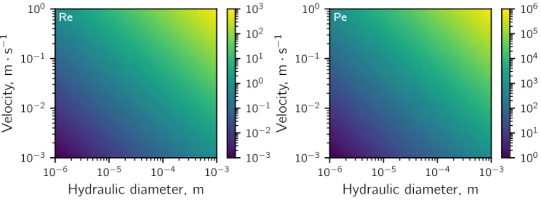
Re 10−6 ₁₀−5 ₁₀−4 ₁₀−3 Hydraulic diameter, m 10−3 10−2 10−1 100 V elocit y, m · s − 1 Pe 10−6 ₁₀−5 ₁₀−4 ₁₀−3 Hydraulic diameter, m 10−3 10−2 10−1 100 V elocit y, m · s − 1 10−3 10−2 10−1 100 101 102 103 100 101 102 103 104 105 106

Figure II.1: Left: Typical numerical values of the Reynolds number for water (ν = 1 · 10−6_{Pa · s) at different hydraulic diameters and fluid velocities. Right:}

Typical numerical values of the Péclet number for small ions in water (D = 1 · 10−9_m2_{· s}−1_).

The Reynolds number (Re) relates inertial forces to viscous forces and is defined as: Re = u L

ν . (II.2)

It gives an indication about the flow regime. Figure II.1 shows values of Re for typical channel diameters and fluid velocities encountered in microfluidics. For Re < 1000 in a straight microchannel the flow is typically laminar, which means that the fluid moves parallel to the channel wall. The flow only becomes turbulent for higher values of Re. Consequently, the fluid molecules are not mixed by convection and diffusion dominates.

(19)

species:

Pe = u L

D . (II.3)

It enables to estimate the necessary channel length that is required to achieve complete mixing. Figure II.1 shows Pe for a solute ion with a typical diffusion coefficient in the order of 1 · 10−9_m2_{· s}−1_{. Assuming a hydraulic diameter of 100 µm and a velocity of 1 mm · s}−1_a

Pe of 100 is obtained. This means that it would take around 100 channel widths (≈1 cm) for the fluid to mix completely. For larger solutes like proteins with slower diffusion coefficients (≈ 1 · 10−11_m2_{· s}−1_{) this can be either exploited to separate objects with higher diffusion}

coefficients or it can be a problem if mixing is desired.[47] _{To mix the fluid faster, the}

channel geometry has to be modified to create a turbulent flow.[80]Another possibility is to segment the flow into droplets. The droplets have internal flow patterns that were found to mix the content with a mixing time that is logarithmically proportional to Pe.[81]

When two immiscible fluids are introduced into a microfluidic channel, the surface tension tries to minimize the surface area between them, while the viscous forces drag the interface downstream. The capillary number (Ca) relates the viscous forces to the surface tension:

Ca = η u

γ . (II.4)

It allows to estimate the droplet radius R ∝ Ca−1_{and if droplets are likely to be created}

or not.[47] For low numbers of Ca droplets will form, while at higher numbers viscosity dominates and tends to form a co-flow of both phases.[82] _{Figure II.2 shows capillary}

numbers for a fluid velocity of 1 m · s−1_.

Ca 10−3 ₁₀−2 ₁₀−1 Surface tension, N · m−1 10−3 10−2 10−1 Dynamic viscosit y, P a · s 10−2 10−1 100 101 102

(20)

Preparation of Microfluidic Devices

Nowadays, microfluidic systems can be prepared from different materials and by various techniques.[83–85] _{The first devices, however, were etched into silicon and glass with the}

help of photolithography.[85–87] _{The high cost associated with these techniques stimulated}

the development of other preparation techniques and promoted the use of other materials, mostly polymers or even paper.[83–86]_{Polymers have the advantage of being relatively cheap,}

available and processable. The probably most used polymer for scientific applications is polydimethylsiloxane (PDMS). It can be cast against a master mold and then be used to prepare a microfluidic device or be used as a mold itself in soft lithography.[88–90]_{The master}

can be prepared in any way e.g. machining or photolithography. For photolithography (Figure II.3), a so called mask is required to create 3D structures from a photoresist. The first step in this procedure is to draw the mask, which defines the microfluidic channel structure, with a computer-aided design program and to print it on a transparent sheet of polymer. In the second step, a flat substrate is coated with a photoresist. After aligning the printed design to the substrate, it is irradiated with light of a certain wavelength to initiate a polymerization reaction in the photoresist. The parts that are protected by ink do not react and can be removed after the polymerization is finished, e.g. by selective dissolution. To obtain the PDMS mold, liquid PDMS monomers are cast against the master and polymerized at elevated temperatures (Figure II.4). The obtained PDMS replica is then usable as part of a microfluidic device or as a mold itself.

Mask Photoresist

Substrate Master

Figure II.3: Photolihographic process. Left: The mask is aligned to the substrate and the layer of photoresist. Center: The assembly after exposure to light. The exposed parts of the photoresist are polymerized. Right: 3D structures are created by dissolving the unreacted photoresist.

Off-Stoichiometry Thiol-Ene-Epoxies

Off-stoichiometry thiol-ene-epoxies (OSTE+) are a relatively new class of polymers for the preparation of microfluidic systems.[91] _{They were developed from the off-stoichiometry}

(21)

Master PDMS

Replica

Figure II.4:Replication molding process. Left: PDMS monomers are cast against the master. Center: After heat exposure PDMS is cured and can be cut free. Right: 3D structures are replicated after demolding the PDMS piece.

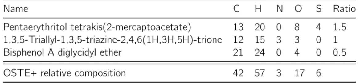
Sweden. The liquid pre-polymer is composed of thiol, alkene and epoxide monomers (Table II.1), a photoinitiator and a photolatent base.[93]_{After mixing, it can be cast against}

a PDMS mold for soft lithography. For OSTE+ the first curing step is initiated by UV radiation and is based on thiol-ene click chemistry.[94] _{The resulting polymer is flexible and}

sticky when touched. In the second curing step the epoxide groups react with the excess thiol groups under the influence of heat and the polymer stiffens when it is cooled down.[93]

The second curing step can be used to bond the OSTE+ to other surfaces via the epoxy chemistry. Before the final curing step, the excess surface thiol groups can also be used for surface modification.[95]

Table II.1: Generic functional groups in the OSTE+ pre-polymer.

Thiol Alkene Epoxide

R S H R CH CH2 R CH CH2 O Droplet Microfluidics

In the following, the most basic ideas regarding droplet microfluidics will be summarized. For more in-depth information, many reviews are available on this vast topic.[96–103]

To generate droplets, two immiscible fluids have to be introduced into one microchannel. This happens usually by applying a direct pressure difference between the inlet and the outlet or by using syringe pumps that drive the fluids at a certain flow rate. The use of two fluids creates new requirements regarding the device material since it should be resistant to both. PDMS, for example, tends to release oligomers or swells when brought into contact with certain organic fluids.[104] _{Another consideration that has to be made beforehand is}

(22)

the phase preference of the used materials. To obtain water droplets in an oil phase, the channel walls should be hydrophobic so that the oil phase wets the walls and the water droplets do not. If the wetting behavior is not sufficient, it can also be influenced by the addition of surfactants.[105,106] _{Adding surfactants or particles also helps stabilizing the}

formed droplets.[105,107] When choosing a surfactant, special care should be taken so that the surfactant does not influence the droplet content.[108]

Active and passive methods can be used for the generation of droplets. While active methods make use of electrical, thermal, magnetic and mechanical controls, passive methods rely on the geometry, the flow rates and the physico-chemical properties of the system alone.[98,99]

The three principle geometries to generate droplets are co-flow, flow focusing and cross flow (Figure II.5). In co-flow, the two phases meet in flow direction (parallel streamlines),

Figure II.5: Examples for different droplet generation geometries for a fluid flow. Left: Co-flow. Center: Flow focusing. Right: Cross flow (T-junction).

while they meet at an angle in cross flow. For flow focusing, an obstruction narrows down the channel to promote the droplet formation.[103] _{The T-junction is the simplest example}

for the cross flow geometry and was used in the first report on droplet generation.[109] _As

predicted by the capillary number, the droplet generation pattern depends on the flow rates, the fluid viscosities and the channel geometry.[110] _{Three principle flow behaviors can be}

observed for the T-junction: squeezing, dripping and jetting (Figure II.6).[97,98,111]

Squeezing is observed at low capillary numbers. The dispersed phase protrudes into the continuous phase and fills the channel. As the distance between the dispersed phase and the channel wall decreases the pressure in the carrier phase increases. When the pressure is larger than the pressure of the dispersed phase, a neck forms and the liquid breaks at this point. This position is referred to as pinch-off position. The formed droplets are highly monodisperse[112] _{and have an elongated shape due to their high volume that is constrained}

by the channel geometry.

Dripping appears when the capillary number is increased and the viscous forces start to dominate the interfacial stabilization of droplets. Droplet break-up occurs close to the junction, but the dispersed phase does not touch the opposite wall before pinch-off. The droplets are also monodisperse but smaller than in the squeezing regime.

(23)

Jetting occurs for high capillary numbers. The dispersed phase is pulled downstream into the carrier phase and breaks into small polydisperse droplets due to the Plateau-Rayleigh instability[113] _{of the liquid thread.}

Figure II.6:Droplet flow behaviours in a T-junction. The carrier phase flows from left to right. The dotted line indicates the pinch-off position. Left: Squeezing. Center: Dripping. Right: Jetting.

For a droplet that flows in a straight channel the shear stress at the channel walls create circulating flow patterns inside the droplet. The patterns are symmetrical and parallel to the flow direction of the droplet. While mixing is promoted along the flow axis, it remains slow and stays dominated by diffusion across the symmetry axis. To overcome this limitation, chaotic advection can be introduced by a winding channel geometry.[81] _{When passing}

the winding channel, the interface between the two droplet halves reorients into the flow direction and the droplet content is folded and stretched, which leads to faster mixing.[81]

The mixing time tmix was found to scale for high Pe as:

tmix ∼

( a dh

u )

log(Pe), (II.5)

where a is the dimensionless droplet length measured relative to the hydrodynamic diameter of the microfluidc channel dh. Mixing times as rapid as ≈ 500 µs have been achieved in a

microchannel with a hydrodynamic diameter of 10 µm at fluid velocities of 400 mm · s−1_.[81]

Such low mixing times allow to decouple mixing and reactivity to probe reaction kinetics.[54]

2.2 Small Angle X-ray Scattering

In the following, some basics regarding SAXS will be discussed that are necessary through-out the manuscript. More details on this topic can be found in specialized articles and books.[33,34,114–116]

X-ray radiation has a wavelength between 0.01 and 10 nm. Upon interaction with matter, it can be absorbed or scattered. Absorption of X-rays depends on the atomic species present in the material and on the energy of the radiation. The mass attenuation coefficient (µ

(24)

describes the property of a material to be penetrated by X-rays of a certain energy. It is tabulated[117] _{for different atoms and is calculated from the linear attenuation coefficient µ}

and the density ρ. To calculate the mass attenuation coefficients of any material (µ ρ)x, the coefficients of its components in their respective mass ratio need to be summed up:

(µ ρ)x = ∑ mi mx( µ ρ)i. (II.6)

The transmitted intensity IT of an incident intensity I0 is:

IT = I0e(−µds), (II.7)

where ds is the sample path length. The transmittance is defined as the ratio of transmitted

intensity over incident intensity:

T = IT

I0. (II.8)

Upon interaction with an atom, the X-ray can also be scattered by its electrons, either with loss of energy (Compton or inelastic scattering) or without energy loss (Thomson or elastic scattering). In elastic scattering, the incident wave causes the electron to emit radiation at the same wavelength. Hence, all the atoms in a particle that scatter the incident radiation emit the scattered radiation at the same wavelength, which enables it to interfere. The interference patterns carry the structural information of the particle.

2Θ q Detector Sample ki ks Beamstop Beam

Figure II.7: Schematic representation of a SAXS experiment showing the incident, the transmitted and scattered part of the beam.

A scheme of a typical scattering experiment is depicted in Figure II.7. The incident beam of wavelength λ hits the sample and propagates until it is absorbed by a so called beamstop, which protects the 2D detector. A beamstop is necessary because the dynamic range of the detector is limited and the incident beam is highly more intense than the scattered part of the beam. The number of scattered photons is measured by the detector as a function of the scattering angle 2Θ. In the SAXS experiment, the magnitudes of the incident and

(25)

scattered wave vectors are equal:

|⃗ki| = | ⃗ks| =

2π

λ . (II.9)

The scattering vector is:

⃗

q_{≡ ⃗}ks− ⃗ki, (II.10)

and its magnitude is:

q ≡ |⃗q| = 4π

λ sin Θ, (II.11)

which has the unit of nm−1 _{and is referred to as the reciprocal space. Combined with}

Bragg’s law:

2d sin Θ = n λ, (II.12)

one obtains:

q = 2 π

d , (II.13)

which links the reciprocal space to the real space d.

Each electron that is illuminated by the X-ray beam has the same contribution to the observed scattering, which is described by the scattering cross section σ. The ratio between the photons that are scattered into any unit solid angle (Ω) per unit time Φs and the total

number of photons per unit time Φ0 gives the differential scattering cross section:

dσ dΩ(q) =

Φs

Φ0. (II.14)

The differential scattered cross section per unit volume, defined as: dΣ dΩ(q) = 1 V dσ dΩ(q) (II.15)

gives the scattering on the absolute scale. To obtain it from the measured intensities, the detector counts I(q, t) need to be corrected for the acquisition time t, the subtended solid angle ∆Ω, the sample thickness ds, the transmission T and the incident intensity I0

I(q) = dΣ dΩ(q) =

1 dsT I0∆Ω t

I(q, t). (II.16)

Depending on the detector, different other corrections have to be applied, e.g. dark current correction for the base read out of the detector.[118] Furthermore, it is necessary to subtract

(26)

background scattering from the sample environment (e.g. solvent, the windows of the sample holder, air) to obtain the scattering pattern of the sample alone.

Calibration standards like silver behenate[119] _{(peaks at q = 2πn/5.84 nm}−1_{) or}

tetrade-canol[120] _{(peaks at q = 2πn/1.58 nm}−1_{) can be used to calibrate the sample-detector}

distance. With a known sample-detector distance and the incident position of the direct beam, the 2D detector image can be azimuthally integrated to yield the scattering pattern as I(q) versus q. The intensity can be calibrated when the intensity of the incident beam can be measured with the same efficiency as the scattered beam or by secondary standards like water[121,122] _{(I(q)=1.6 · 10}−2_cm−1 _{for q < 4 nm}−1_{), Lupolen}[123] _{(I(q)=6 cm}−1 _for

q = 0.35 nm−1) or calibrated glassy carbon[124,125].

⃗ rj ⃗ rj+1 ⃗r ⃗ ks ⃗ ki 2Θ Sample

Figure II.8: Scattering of two points. Their relative positions are characterized by ⃗r. The interference of the scattered waves of two points can be described in terms of its phase difference ∆φ. With the relative position of the scatterers ⃗r = ⃗rj − ⃗rj+1 (Figure II.8), the

phase difference of the scattered waves is:

∆Φ = ⃗r (⃗ki − ⃗ks) =−⃗r ⃗q. (II.17)

Since X-rays are scattered by electrons, a pair of scattering objects can be described in terms of its scattering length density ρ(⃗r):

ρ(⃗r) =∑ρi(⃗r) bi, (II.18)

where ρ(⃗r)i is the local density of scatterers of type i and the Thomson scattering length

b = e2/(4π ϵ0m c2) = 2.82· 10−15m.

Under the assumption that the scattering of an object is independent of the scattering by other scatterers (Born approximation), the local scattered amplitudes are added up:

(27)

A(q) = ˆ

V

ρi(r )e−i q ⃗rd⃗r. (II.19)

The scattered amplitude is the Fourier transform of the scattering length density and the scattered intensity per unit volume V is:

I(q) = A(q) A∗(q)

V . (II.20)

With Equation II.19 the intensity can be written as: I(q) = 1 V ˆ V ˆ V ρi(⃗r)ρi(⃗r′)e−i q(⃗r−⃗r′)d⃗r d ⃗r′. (II.21)

With the correlation function:

γ(⃗r) = 1 V

ˆ

V

ρi(⃗r′) ρi(⃗r + ⃗r′) d ⃗r′, (II.22)

the scattered intensity can be expressed as: I(q) =

ˆ

V

γ(⃗r)e−i q ⃗r_d⃗r, _(II.23)

highlighting the fact that the scattered intensity is the Fourier transform of the spatial correlation function.

To describe the observed scattering of monodisperse centrosymmetric particles, the scatter-ing intensity can be written as:

I(q) = N V2∆ρ2P(q) S(q), (II.24)

where N is the number of particles per unit volume, V is the volume of the particle, ∆ρ2

is the relative scattering length density, P (q) is the form factor and S(q) the structure factor. ∆ρ2 _{describes the contrast between the scattering object and the background and}

determines the scattering power. The form factor P (q) is the result of the interference of all the scattered photons from a single particle and is typical for its shape. If there are several particle shapes present, the observed scattering pattern will be an average of the form factors. The structure factor S(q) describes the interparticle interactions. To observe the form factor of monodisperse particles the system has to be dilute, so that no particle-particle interactions are present (S(q) ≈ 1). For a more concentrated system, the

(28)

interference pattern will contain information about neighboring particles, too. A decrease in intensity is generally indicative of a repulsive interaction, while an increase indicates attraction or particle aggregation. When such bumps develop into peaks it indicates highly ordered structures. The order of the peak positions enables to identify the symmetry of such (crystalline) structures.

2.3 Combining SAXS and Microfluidics

For the combination of SAXS and microfluidics, some implications arise from the equations above. First, the attenuation by the device material and the path length of the beam through this material should be small to obtain a strong signal from the sample. Second, the number of scattered photons depends on the scattering volume. The optimum sample thickness is 1/µ and yields a transmission of T ≈ 0.37. For water, this path length is rather large (1 mm at 8 keV) compared to the channel size in microfluidic devices. Therefore, the channel depth should be optimized to improve the signal. Third, the number of scattered photons depends on the number of incident photons. Thus, the photon flux of the beam should be rather high to compensate the non-optimum path length in microfluidic channels. A high photon flux is also particularly important for the combination of droplet microfluidics and SAXS, since the isolation of the droplet signal requires relatively short acquisition times. Overall, these requirements make it necessary to use a high intensity X-ray source, e.g. a synchrotron facility. Additionally, the beam cross section has to be small enough to collect the signal of the channel without any contribution from the device bulk material. Otherwise, parasitic scattering from the channel interface might be observed.

2.4 Isolating the Droplet Signal

In the following, some thoughts on how to isolate the scattering pattern of droplets from the carrier phase are discussed.

The microfluidic device generates a segmented flow of oil and water (Figure II.9). For a given water to oil flow rate ratio the length of the water segment lw is constant. During

the experiment the water droplets pass the X-ray beam, which is characterized by its length lb along the channel axis. To isolate the signal of the droplets:

(29)

lw la

lb

Figure II.9:Droplet generation in a microfluidic device in the path of a rectangular X-ray beam. The droplet length lw, beam length lb and acquisition length la are

indicated. The beam is shown as solid white rectangle, while the broken white rectangle shows the part of the droplet that already moved through the beam during the acquisition time.

has to be fulfilled, otherwise lb will never be completely filled by the water segment. During

the acquisition time ta, the droplets move with a velocity v through the channel. Thus, the

acquisition time corresponds to an acquisition length la over which the signal is collected:

la = ta· v. (II.26)

To optimize the acquisition time, the shorter dimension of an asymmetric beam should be perpendicular to the flow direction. The acquisition length for which only water signal is obtained is:

la ≤ lw− lb. (II.27)

By choosing a la that is smaller than lw, the probability to collect the signal of the droplet

alone increases and several patterns of the same droplet can be acquired for la≪ lw. The

frequency of acquisition fa can be equal to, lower or higher (Figure II.10) than the droplet

frequency fd. However, for fa = n· fd (n ∈ N) the acquisition should be synchronized with

the passing droplets. For this case, a phase shift between the acquisition and the passing droplets might result in a convolution of the droplet and carrier phase patterns or patterns that are only from the carrier phase. Figure II.10 depicts a typical experimental sequence. The frequency of acquisition is higher than the frequency of the droplets. The acquisition time (∝ la) is shorter than the droplet residence time in the beam (∝ lw). As a result

there are three different cases (Figure II.11): i) patterns from the oil phase alone, ii) mixed scattering patterns from oil and droplet, and iii) patterns of the droplets alone.

(30)

time

signal

beam

oil droplet

Figure II.10: Example for an acquisition frequency that is higher than the droplet frequency. The obtained scattering patterns are isolated droplet and oil phases and mixtures of both.

Figure II.11: The three potential acquisition possibilities in droplet microfluidics. The rectangle represents the probed area by the X-ray beam. Left: Only the scattering of the oil phase is acquired. Center: The scattering of oil and droplet is acquired. Right: Only the scattering of the droplet phase is acquired.

3 Materials and Methods

3.1 Microfluidic Device Fabrication

WBR/Si Masters

WBR/Si masters were prepared by laminating layers of dryfilm (50 µm thick WBR2050 and 100 µm thick WBR2100, Dupont) with a hot roll laminator onto a Si wafer (Sil’Tronix Silicon Technologies). After the lamination, microstructures were created by photolithography. To create a photomask the device structure was designed with the help of a computer-aided design program and printed on a flexible polyester film by a commercial service (JD Photo Data).

Before laminating the wafer it was degreased with acetone (99 %, Honeywell) and blow-dried with pressurized air. The first film layer was roughly cut to size and the protective polyethylene layer was removed by using sticky tape, before placing the wafer on a supporting metal plate (Cu, 1 mm thick). Then, the dryfilm was aligned to it with the unprotected

(31)

side facing the wafer. To reduce wrinkling of the film, the dryfilm was brought into contact with the metal support on the advancing side of the wafer before starting the roll laminator and the film was kept under tension during the lamination (Figure II.12). The lamination temperature was 85◦_{C and the lamination speed was approximately 24 mm · s}−1_{. After}

lamination, the wafer was turned upside down and the excess dryfilm was removed. To apply a second layer of dryfilm, the protective polyester layer on top of the wafer-WBR stack was removed by using sticky tape and the procedure was repeated. The adhesion between the film and the substrate was improved by baking the piece over night at 60◦_{C in an oven.}

After the item reached room temperature, the protective polyester layer was removed by using sticky tape, a photomask was aligned and brought into contact with the film. The assembly was then exposed to UV light for 20 s at 48.8 mW · cm−1 (365 nm, UV-Kub 2, Kloé). Before development, the excess of dryfilm was removed with a razor blade and it was baked at 100◦_{C for 60 s on a hot plate (C-MAG HP 10, IKA). After cooling down, it}

was developed by applying a stream of 1 % K₂CO₃ solution with a peristaltic pump (101U, Watson Marlow) until no undeveloped film was visible anymore. To finish the development it was washed with tap water and carefully blow dried with pressurized air.

pull gently

WBR

Si Cu

Figure II.12:Lamination of WBR dryfilm onto a Si wafer with a hot-roll laminator. By gently pulling the dryfilm during lamination it is kept under tension and the final laminate is wrinkle free.

PDMS Molds and Flat

PDMS negatives and flats were prepared by mixing PDMS elastomer base with its curing agent in a 10:1 ratio (Sylgard 184, DOW). After thorough mixing, the mixture was poured on the master and left under reduced pressure to remove air bubbles. The polymer was cured overnight in an oven at 60◦_{C. The PDMS pieces had to be relatively thin to fit into}

(32)

piece.

Off-stoichiometry Thiol-ene-epoxy Device

Off-stoichiometry thiol-ene-epoxy (OSTE+) pre-polymers (OSTEMER 322, Mercene Labs) were mixed in the indicated ratio (1.00:1.09) with a vortex mixer and shaked by hand until all haziness disappeared. Before use, it was left to rest until no air bubbles were visible anymore. OSTE+ was then poured on the PDMS mold and covered by another piece of PDMS, stabilized by a glass microscopy slide. By applying pressure, the excess OSTE+ was removed and recovered. To remove air bubbles that appear during the pouring step and are trapped on the design features, the PDMS molds were placed under reduced pressure beforehand and the filled mold stack was left alone until no bubbles were visible anymore. The assembly was then irradiated with approximately 24.4 mW · cm−1 _{for 120 s (365 nm,}

UV-Kub 2, Kloé). Afterwards, the PDMS mold was removed and the UV-cured OSTE+ carefully peeled off. Removing excess OSTE+ on the edges with sticky tape proved to facilitate the demolding. The flexible piece of OSTE+ was then placed on a flat sheet of polytetrafluoroethylene (PTFE) with the structured part facing down and cured in an oven at 90◦_{C overnight. Access holes were machined into the fully cured piece with a bench-top}

drill. To align the drill with the device and to obtain reproducible hole distances a PMMA template was used. The cured and drilled piece was then rinsed with alcohol, blow dried with pressurized air and cleaned with sticky tape. Afterwards, it was aligned and bubble-free laminated onto a UV-cured flat piece of OSTE+ at room temperature. The assembled piece was then transferred onto a PTFE sheet and again cured at 90◦_{C overnight in an}

oven. The process is sketched in Figure II.13.

Polyimide Composite Devices

To decrease the wall thickness of the device and the OSTE+ contribution to the wall, a commercial polyimide foil (Kapton, DuPont) with a thickness of 25 µm was used as wall material. The preparation protocol is similar to the pure OSTE+ device. The OSTE+ pre-polymer was mixed as described above and poured on the PDMS mold. It was then covered by a polyimide foil and a microscopy support slide, which were pressed against the bottom part to remove excess OSTE+ prepolymer. Then, the assembly was turned so that the polyimide foil was below the OSTE+ prepolymer and cured with UV light (365 nm, 24.4 mW · cm−1_{, 120 s, UV-Kub 2, Kloé). Note that if the polyimide foil is between the}

(33)

OSTE+ Glass PDMS 1. UV 2. 90◦_C 3. drilling UV 90 ◦_C A B C

Figure II.13:OSTE+ device fabrication. A: PDMS molds are consecutively filled with OSTE+ pre-polymer, aligned, exposed to UV and demolded. The flexible OSTE+ is then cured at 90◦_{C and access holes are drilled into the material.}

B: PDMS molds are consecutively filled with OSTE+ pre-polymer, aligned, exposed to UV and demolded. C: The flexible bottom part is aligned to the rigid top part and cured at 90◦_C.

(34)

prepolymer and the light source no curing occurs due to absorption by polyimide. Afterwards, the OSTE+/polyimide is demolded and access holes were punched with a biopsy puncher (Ted Pella). To obtain reproducible hole patterns, a template was printed on paper and aligned to the device before punching. The device was closed by bonding the OSTE+ part to a second polyimide foil at 90◦_C.

Surface Modification of OSTE+

To increase the hydrophobic character of OSTE+ surface, it was hydrophobized by flushing the channels with a solution of a fluorosilane polymer (Novec 1720, 3M) before putting it on a hot plat at 110◦_{C for 30 min. The process was repeated for a total of three times.}

Fabrication of Polydimethylsiloxane Devices

PDMS devices were directly obtained from WBr/Si by mixing PDMS elastomer base with its curing agent in a 10:1 ratio (Sylgard 184, DOW), pouring the prepolymer onto the master and degassing it under reduced pressure. The polymer was cured in an oven over night at 60◦_{C. To increase the hydrophobic character of the PDMS surface it was hydrophobized}

with the same procedure as the one described for OSTE+.

3.2 Characterization of OSTE+ Microfluidic Devices

Surface Homogeneity and Channel Height

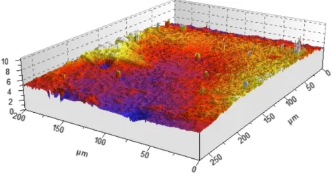
The channel height of the WBR master and the OSTE+ device, and the surface of the OSTE+ were probed by a white light interferometry microscope (smartWLI basic, Gesellschaft für Bild- und Signalverarbeitung (GBS) mbH) and analyzed by commercial software (MountainsMap, Digital Surf).

Device Thickness

The total thickness of one finished and one half-finished device was measured at different locations with a digital micrometer (293-521 N, Mitutoyo, precision of 1 µm) with a probing head diameter of 6.35 mm2_.

(35)

3.3 Microfluidic experiments

Materials

Oils. Several oils were tested as inert carrier phase. FC-40, FC-70, FC-3283, perfluorode-caline, 3-octanol, hexadecane and light mineral oil were acquired from Sigma-Aldrich.

Surfactants. To stabilize the droplets and to improve the wetting behavior of the oil phase several surfactants were tested. Span 80 (sorbitan monooleate) was acquired from CRODA and used in combination with hexadecane and light mineral oil. ABIL EM 90 was acquired from CRODA and used in combination with light mineral oil.

Reactant Solutions. Cerium nitrate (Ce(NO3)3, Sigma-Aldrich) and oxalic acid (H2C2O4,

Sigma-Aldrich) solutions of various concentrations were prepared with high purity water (18.2 MΩ · cm) and a binary mixture as solvent. The binary solvent consisted of high purity water and 1,2-propanediol (Sigma-Aldrich) in a 25:75 ratio by weight.

Gold Nanoparticles. Gold nanoparticles were produced from a reverse Turkevich method following the protocol described by Siveraman et al.[126] _{250 µL of aqueous 25.4 mM HAuCl}

4

solution is added rapidly to 24.75 mL of 5.2 mM boiling citrate solution under vigorous stirring. Boiling is stopped after 250 s and the solution is let without stirring for 12 h before being used. The nanoparticles are characterized by SAXS and TEM (see Appendix A) and have a diameter of 9.4 ± 1.0 nm.

Fluid control

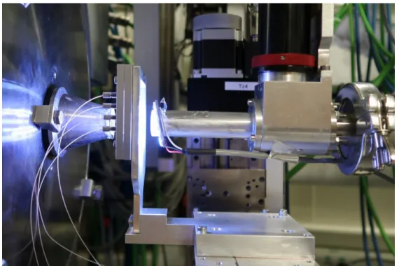
The microfluidic device was connected to computer controlled (neMESYS UserInterface, Cetoni) syringe pumps (neMESYS system, Cetoni) via a customized device holder (ICH-01K, IMT). Polyether ether ketone (PEEK) tubing was connected to gas tight syringes (SGE Analytical Science) by Luer adapters on one side and to the device holder by hollow screws with a PTFE gasket on their tip on the other side (Figure II.14). To use the device holder in the X-ray scattering experiments an adapter was machined from stainless steel (Figure B.1).

(36)

Figure II.14: Left: IMT device holder with tube connector. Right: IMT tube connector with PTFE gasket.

Preliminary Experiments on Droplet Formation and Reactant Mixing

Observations were made through a microscope (IMT-2, Olympus) with a mounted and computer controlled (Phantom Camera Control 2.2, Ametek) high speed camera (Phantom v7.3, Vision Research). Droplets were generated by uniting three streams of water and feeding it into a T-junction with an immiscible phase. The flow rates, the wetting behaviour, and the droplet pinch-off were optimized. To observe reactivity in the formed droplets, two of the three water streams were substituted by a stream of cerium nitrate and oxalic acid solution (Figure II.15). The two channels were separated by a stream of solvent in the center channel to avoid reactivity before the mixing part of the device. The droplets were then allowed to mix in a passive serpentine mixer and to age in a 24 cm long channel before being collected. mixing aging A C B Mixing Aging A B C

Figure II.15: Schematic representation of the microfluidic device. A T-junction into which an oil phase and three aqueous phases are fed. The generated droplets mix in a passive serpentine mixer and age in a long channel. By varying the content and flow rate of the channels A, B and C, the droplet content is varied.

(37)

Estimation of the Mixing Time

Observations were made through a microscope (CKX41, Olympus) with a mounted and computer controlled (Micromanager, Open Imaging) camera (pco.edge 5.5, PCO). To estimate the mixing time an aqueous solution of a fluorescent dye (fluorescein, Sigma-Aldrich) was fed to the device and mixed with water in water-in-oil droplets. Fluorescence was initiated by a UV-source (U-RFLT50, Olympus) and the traveled distance to reach a homogeneous fluorescence in the droplet was observed.

3.4 X-ray Scattering Experiments

X-ray scattering experiments were performedi) at the SWAXS Lab Saclay on a Xeuss 2.0 laboratory beamline (Xenoxs) at a photon energy of 8.04 keV with a Pilatus3 R 1M detector (Dectris) at a sample detector distance of 42.4 cm and ii) at the small and wide angle X-ray scattering (SWING) beamline of the SOLEIL synchrotron facility in France, at photon energies of 12.00 and 16.00 keV with a Eiger 4M detector (Dectris) at a sample detector distance of 52.2 and 616.5 cm. Sample detector distances were verified using tetradecanol as calibrant.

X-ray Transmittance of OSTE+ and its Linear Attenuation Coefficient

Calculations were made with the help of xraylib,[127] _{values for the X-ray mass attenuation}

co-efficient are listed in different databases like the NIST Standard Reference Database 66.[117]

Standard Data Treatment

Each raw scattering pattern was masked and azimuthally averaged to yield the scattering curve I(q). The intensity was normalized by the solid angle, the acquisition time and the transmitted flux. After background subtraction, the intensity was normalized by the sample thickness and brought to absolute scale by calibration measurements of Lupolen or water.

Material Aging

In order to investigate on the impact of X-rays, OSTE+ was repeatedly irradiated at 16.00 keV with a 50 µm × 400 µm (vertically × horizontally) beam for 500 ms and a gap

(38)

time of 250 ms between each individual acquisition, for a total irradiation time of 500 s. The same procedure was applied to OSTE+ that was additionally cured at 150◦_{C for seven}

days before X-ray irradiation.

Data Treatment for In-situ X-ray Scattering Experiments

A custom Python 3 code was developed and used for data treatment. The nexusformat†

package was used to read data from the Nexus data files, obtained from the SWING beam line. Each frame was radially averaged with the help of the pyFAI[128]‡ _{package and}

normalized by the solid angle, the acquisition time and the transmitted flux. For static samples, several frames were averaged to give a single 2D data file. Data from droplet experiments was analyzed regarding the variation in scattering. Oil and droplet phase have different scattering curves and intensities. A segment of the scattering vector was defined in which the intensity of each curve was averaged. The data was then categorized based on threshold values, rejecting a certain percentile of the data and assigning the remaining data as droplet or oil phase based on their value. Data where the signal of oil and droplet is mixed has an intermediate value and was rejected. After sorting the data, each phase was separately averaged to yield one data file. If possible, the background scattering was subtracted and the data was normalized by the channel thickness and a normalization factor to obtain the absolute scattering intensity. The full code is provided in Appendix C.

4 Results and Discussion

4.1 Microfluidic Device Fabrication

The process to develop a protocol for the preparation of OSTE+ devices with a suitable thickness in a reproducible way was rather time consuming and challenging. In the following, some of the key choices in the described protocol are discussed.

Si Master

The first masters were prepared with SU-8 (MicroChem) as photoresist. After adapting the initial device design to the requirements of the experiment, it became apparent that SU-8

†_{https://github.com/nexpy/nexusformat} ‡_{https://pyfai.readthedocs.io}

(39)

has some drawbacks, i.e. for the preparation of thick layers. In contrast to SU-8, WBR dry film can be stacked and gives access to thick layers of photo resist in a reproducible fashion. However, WBR has some drawbacks, e.g. its relatively poor adhesion properties. To improve the adhesion to the substrate it was useful to extend the post-lamination bake overnight at 60◦_{C instead of 20 min only, as suggested in the data sheet. A finished master}

is depicted in Figure II.16.

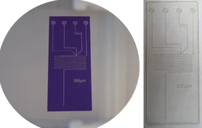
Figure II.16: Left: WBR/Si Master. Right: Finished OSTE+ device.

PDMS Molds

The use of PDMS molds instead of directly using a Si master has several benefits. First, it is less time consuming to replace a PDMS mold than a Si master and PDMS molds can easily be prepared from the masters. Second, PDMS is transparent to visible and UV light, which allows spotting potentially trapped bubbles and enables the OSTE+ prepolymer curing by UV light. Third, the porosity of PDMS facilitates the elimination of trapped air bubbles after filling in the OSTE+ pre-polymer by degassing the PDMS mold before use. Finally, PDMS is flexible and simplifies the demolding after the UV curing step. However, the elasticity of PDMS is a problem during the stacking step of the molds to give a fixed height (Figure II.13). Without support, the PDMS roof tends to collapse onto the chip design under pressure. This problem can be addressed by supporting the PDMS mold with a glass slide. For ease of use, the glass slide can be permanently bonded to the PDMS piece by plasma treatment.

(40)

OSTE+ Device Preparation

There are several considerations in the presented protocol that deserve to be discussed. i) Using two molds for the preparation of the device parts, allows to prepare devices

with different designs and wall thickness simply by switching the bottom or top mold. In a one-mold approach, each design would have a fixed wall thickness and would require the preparation of a new master in a two-step photolithography process. The first step would define the wall thickness, while the second step creates the design. Additionally, a flat piece of OSTE+ needs to be prepared to close the device. Thus, the mold that defines the wall thickness can be used for both pieces.

ii) Instead of removing excess OSTE+ prepolymer after aligning and pressing the molds together, the molds could be aligned beforehand and then be used for injection molding[78] _{or they could be filled by capillary forces.}[129] _{Both alternative approaches}

were tested and should be viable after adaptation, but were not used further. iii) After filling the molds with liquid pre-polymer, a UV curing step follows to polymerize

the material. The irradiation time was rather long and the lamp was only operated at half of its maximum power to obtain a complete reticulation without generating too much heat, which would trigger the second curing step.

iv) The final wall thickness of 200 µm that is imposed by the PDMS mold. For thinner walls, the structured part teared easily during demolding after the first curing step. One solution to reduce this thickness is the use of a thin X-ray compatible wall material like polyimide foil or other commercial foils. Another would be to pre-fabricate thin, fully cured sheets of OSTE+ as support material and to use them instead of the second mold.

v) OSTE+ sticks to many materials thanks to the epoxy groups. These groups are activated during the heating step and some sort of support is necessary to hold the OSTE+ items. Although OSTE+ should not adhere to aluminum, the thin devices could not be removed without damaging them. Thus, a sheet of PTFE was used as support material.

vi) The first half of the chip was fully cured before the device was assembled, since drilling into fully cured OSTE+ gave cleaner holes than using biopsy punchers on only UV cured pieces. Punching the holes also creates sticky debris, which is tricky to remove afterwards. The debris from machining the fully cured workpiece is not sticky and can be easily removed by pressurized air and sticky tape. A drawback of fully curing

(41)

OSTE+ before assembling the final device is that it limits the choices for surface modification. OSTE+ that is only cured by UV can easily be surface modified to show more hydrophobic or more hydrophilic behavior.[95] _{However, modification of}

the whole piece, instead of the channels only, prevents bonding in the heat-curing step due to the loss of the respective functional groups. The bonding capacity can be retained by adding allyl glycidyl ether to the modification cocktail. The downside of using allyl glycidyl ether is its acute and reproductive toxicity, and its mutagenic and carcinogenic properties. Due to these safety concerns in combination with local conditions and limitations in the laboratory, the surface modification was carried out after the device was assembled and fully cured.

vii) The alignment and lamination of the two OSTE+ parts are the probably most delicate steps in the preparation of the device. To achieve a bubble-free assembly the two parts can be laminated either by a roll laminator or by applying the necessary pressure by hand. Another, untested method might be the use of a bench-top press. Whatever the method, it is important that there are no remaining trapped particles or air bubbles. Both might result in an unusable device after the final bonding step.

Polyimide Composite Devices

A polyimide/OSTE+ composite device is depicted in Figure II.17. In contrast to the devices that are made of OSTE+ only, the structured part of the polyimide composite devices cannot be cured before finishing the device, otherwise the OSTE+ layer would lose its binding capacity with the second polyimide layer. Since the structured part is not fully cured, the access holes cannot be drilled, but have to be punched. However, this is less of a problem, since the layer thickness of OSTE+ is lower and almost no debris is formed while using biopsy punchers to create the holes. A similar manufacturing approach has been recently reported in literature.[25]

4.2 Characterization of OSTE+ Microfluidic Devices

Surface Homogeneity and Channel Dimensions

White light interferometry microscopy was used to probe the surface roughness of the finished device and the channel height of the master and finished device. The channel width in a finished device was probed by bright-field microscopy. As can be seen in Figure II.18, the